

Abstract
Understanding the interaction of atoms and molecules with an intense laser radiation field is key for many applications such as high harmonic generation and attosecond physics. Because of the non-perturbative nature of strong field physics, some simplifications and approximation methods are often used to shed light on these processes. One of the most fruitful approaches to gain an insight into the physics of such interactions is the three-step-model, in which, the electron first tunnels out through the barrier and then propagates classically in the continuum. Despite the great success of this and other more sophisticated models there are still many ambiguities and open questions, e.g. how long it takes for the electron to tunnel through the barrier. Most of them stem from the difficulties in understanding electron trajectories in the classically 'forbidden' zone under the barrier. In this theoretical paper we show that strong field physics and the propagation of electromagnetic waves in a curved waveguide are governed by the same Schrödinger equation. We propose to fabricate a curved optical waveguide, and use this isomorphism to mimic strong field physics. Such a simulating system will allow us to directly probe the wave-function at any point, including the 'tunneling' zone.
Export citation and abstract BibTeX RIS
1. Introduction
The interaction of atoms and molecules with intense lasers is a key for a rich set of physical phenomena associated with attosecond physics processes such as high harmonic generation [1–4] (HHG), above threshold ionization [5] (ATI), laser induced diffraction imaging [6] (LIED), laser induced inner-shell excitation [7, 8] and steering electrons in molecules [9]. The simple-man model, known also as the three-step-model [10, 11] is a good starting point to gain an insight into these high-field processes. In this simple-man model, at the first step, the laser field is considered to be strong enough to deform the atomic potential, which allows the electron to tunnel out from the atom through the formed barrier [12–14]. In the second step, the motion of the electron is treated classically by taking into account only the laser field, and assuming that the electron emerges at the continuum with zero velocity. In this second step, depending on the time at which the electron emerges at the continuum, some electron trajectories are running away from the parent ion, while other trajectories are running towards it, leading to a re-collision with the parent ion. In the last step, we consider the re-collision process of the electron with the parent ion which can split into a few possible channels: (a) recombination into the ground state while releasing the excess energy in the form of electromagnetic radiation (HHG), (b) elastic scattering (ATI, LIED), and (c) inelastic scattering (atomic/molecular excitation and non sequential double ionization) [7, 8].
Among these three steps, the tunneling ionization is probably the most complicated to understand, which is why it still contains many open questions e.g. when exactly the electron leaves the atom, at what time it enters into the classical forbidden zone under the barrier, how long it takes to tunnel through the potential barrier, what the electron velocity is inside the 'forbidden' zone and right at the exit point from this 'forbidden' zone [15]. The problem arises mainly because of the evanescent nature of the wave-function under the potential barrier. In 1932, MacColl [16] studied the time which may be associated with the tunneling of a particle through a potential barrier. Since then, many efforts have been directed toward defining [17–19] and measuring [20–22] tunneling times. Recent efforts [23–26] try to resolve the related open question of how long it takes for the electron to tunnel through the distorted Coulomb potential and to emerge in the continuum. Agreement on a suitable theoretical definition of tunneling time and the interpretation of experimental results is still lacking [25, 26]. Part of the reason for these difficulties comes from the fact that we cannot probe the electron wave-function, or any related physical observable, inside the tunneling zone. The best we can do is try to infer it indirectly from the spectrum of the HHG or the photoelectrons [23, 24]. We can of course calculate the electron wave-function under some simplifications, or solve numerically the time dependent Schrödinger equation. Having the electron wave-function as a function of time, we can 'put' a virtual probe [27] inside the tunneling zone to extract the relevant physical quantities. However, questions regarding the accuracy of the various approximations to describe reality, still remain open.
In this paper we identify the analogy between an atom in a strong external field and a curved optical waveguide. More specifically, we show that both the atom in a strong field and the electromagnetic wave inside a curved waveguide are governed by similar Schrödinger equations. We propose to use this analogy to fabricate a curved optical waveguide, and to use a real probe [28] to directly measure the electromagnetic wave. In that way we can learn what would be the electron wave-function under the analogous strong-field conditions. We further discuss the similarities between electron trajectories and optical rays, and propose to measure directly the optical rays, thus, gaining an insight into electron trajectories and the above-mentioned open questions.
2. Atom in strong field versus curved waveguide
In optics, it is well known that the paraxial approximation to the Helmholtz wave equation obeys the (2+1)-dimensional Schrödinger-like equation:  (see details in the
  axis , i.e. the direction of the beam propagation, plays the role of time in the Schrödinger equation and
  plays the role of
  in the Schrödinger equation. Because of this similarity, many of the solutions to the Schrödinger equation appear also in optics. For example, the transverse electromagnetic beam profile inside a step index fiber, or in a parabolic index fiber, is the same as the wave-function of a particle in a finite square well potential or that of a harmonic oscillator, respectively. Another example is the diverging Gaussian beam, which has the same wave-function as that of a free particle, with a finite initial width. In this isomorphism, the electromagnetic field in a waveguide is analogous to the electron's wave-function in an atom. It is therefore very tempting to adopted this analogy and use optics to mimic the electron wave-function under the action of a strong external field. The advantages of such an approach are two fold: (a) we are not doing any approximation, (b) we can physically probe the electromagnetic field [28] at any point, including the 'under the barrier' zone. The main problem of how to incorporate the 'time'-dependent external strong 'field' into this optical simulator ('time'-dependent means z-dependent) still remains. In the following section we show how we can do exactly that, by imprinting the time dependent strong field into the z-dependent curve of the simulating waveguide.
We start by writing down the non-relativistic time dependent Hamiltonian in the dipole approximation and define a canonical transformation into a new set of coordinates:


Here,  . We can also designate the instantaneous 'kinetic' energy of q(t) as
  . With this canonical transformation, the new Hamiltonian is:

Hamiltonian (3) describes a particle that is placed in the same potential as in the original Hamiltonian, but this potential is oscillating in time, following the motion of  . (It is worth noting that the solution for the Schrödinger equation in the new coordinates for a free electron, subjected to the radiation action, immediately yields the Volkov states [29].)
Next, we examine what insight we can gain by adopting the transformed coordinates. Figure 1(a) shows a finite square well potential in the new coordinates (equation (2a)) as a function of time. If we take the analogy between a square well potential and a step index waveguide, figure 1(a) also describes a curved waveguide. The advantage of moving to the new coordinates is now clear: it allows us to extend the analogy and incorporate the coupling to a strong external field, by imprinting it into the geometry of the waveguide. To put the time dependent potential and the z-dependent refractive index on an equal footing in figure 1(a), we draw both with dimensionless time and lengths according to the following scaling:  ,
,  ,
,  ,
,  (see the
  is the wave vector in the waveguide clad. As a result of the waveguide bending, some light is able to escape from the waveguide. This process is called bending losses in optical waveguides and we show in the following section that this process is analogous to the tunnel ionization of an atom in a strong field. Figure 1(b) gives some intuition to the bending losses process within the geometrical optics limit. A guided mode in a rectangle step index waveguide may decompose into two plane waves, which are propagating with the same longitudinal wave vector kz and two opposite transverse wave vectors
  . These plane waves are hitting the waveguide walls at angles which are above the critical angle for total reflection. Therefore, the plane waves are transversely bouncing back and forth between the waveguide walls without any losses. When the waveguide is bent, provided that the bending is strong enough, at some point the angle of incidence of the plane wave goes below the critical angle for total reflection and part of the wave is transmitted through the waveguide walls. Next we discuss in more details the similarities between tunnel ionization and bending losses.

Figure 1. (a) Shows the finite square well potential as a function of time in the  coordinates (equation (2a)) (time unit
  , length unit
  ), or a curved step index waveguide (
 coordinates, length unit
  ). The blue doted line marks the translation of the potential
  . Therefore, the local radius of curvature is R is equivalent to
  (see text below), i.e. inversely proportional to the electric field. (b) Zoom-in of the black doted square of figure 1(a). Two optical rays bouncing back and forth between the waveguide walls due to total reflection. Because of the bending, at some point the incidence angle goes below the critical angle and the rays may escape the waveguide according to Snell low.
Download figure:
Standard image High-resolution image2.1. Bending losses in optical fibers
The theory of bending losses in fiber was developed in the mid 1970s. Here we present only the basic ideas and refer the reader to those early works for further details [30–33]. We start, for simplicity, with a straight step index waveguide, where the waveguide width is L, the refractive index within the waveguide is n2 and the ambient refractive index is  (
( ) (see figure 2(a)). The electromagnetic waves have an angular velocity ω and obey the Helmholtz wave equation, both inside and outside the waveguide

Here s = 1, 2 stands for zone 1 or 2 (outside or inside the waveguide). The solutions in the two zones may be written as: 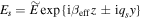 . Inserting these solutions back into the Helmholtz equation we get:

There is a critical wave vector  , beyond which, q1 in the ambient zone becomes imaginary, the wave becomes evanescent in the clad and confined to the core. When the waveguide is bent with a radius of curvature R, we may assume that the fiber mode remains the same as the mode of the straight waveguide, provided the radius of curvature is much larger than the waveguide width. To maintain the same pattern of the mode in the bent waveguide we assume that we can write the wave as
  (see figure 2). Now, the tangential wave vector
  depends on the radius:
  . Replacing
  in equation (5) with this tangential local wave vector we get:

We note that there is a critical distance  from the waveguide center, beyond which, the transverse wave-number
  becomes real again and the waves cease to be evanescent.
Figure 2. Schematic drawing of a straight and a bent fiber. R is the bending radius of curvature, r', the radial distance from the center of the waveguide. To maintain the mode pattern in the bent fiber we assume that the wave is in the form of  . At
. At  the wave is bound to the waveguide and q1 is purely imaginary. At
  , q1 becomes real and the wave ceases to be an evanescence wave.
Download figure:
Standard image High-resolution image2.2. Bending losses versus adiabatic tunnel ionization
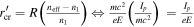
In this section we would like to compare bending losses and tunnel ionization. We start our comparison with the tunneling rate in the adiabatic approximation. There are many ways to calculate the tunneling rate in the adiabatic approximation which give many expressions. However, for exponential accuracy, they are all the same and differ only in the pre-exponential term. Here we give the famous Ammosov–Delone–Krainov [34] (ADK) ionization rate as a reference, though, we are most interested in the exponential term.
The tunneling rate according to the ADK solution is:
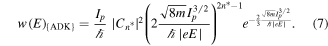
Here,  is the ADK ionization rate as a function of the external electric field,
  ,
, 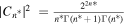 , Z is the net resulting charge of the atom and
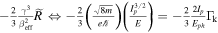
  is the gamma function. Our next step is to compare the ADK ionization expression with the expression of the bending losses. As is the case with the tunneling ionization, there are many expressions for bending losses rates, but for exponential accuracy, they are all the same. Here we present the results obtained by Marcuse [32] as a representative expression

Here,  is the bending loss rate as a function of bending radius R;
  is the waveguide width,
  in equation (5),
 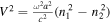 . To compare equation (7) with equation (8) we have to relate the radius of curvature R to the external electric field E. For that purpose we can take a closer look at figure 1(a) which describes a potential well in the transformed coordinate
  In this system of coordinates, the potential well follows a curve that is given parametrically by
  where
where  and
and  . Therefore, the instantaneous radius of curvature of this 'waveguide' is given by:

Throughout the text,  means equivalent quantities.
Using again the analogy between the Helmholtz equation and the Klein–Gordon equation we get: 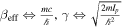 (
( which is exactly the exponential term in equation (7) (
 is the Keldysh parameter). By recognizing that
  and
and  (
( , exactly what one would expect to be the tunneling exit point. It is worth also commenting on the power law of
  or E in the pre-exponential terms in equations (7) and (8). If we take for example the hydrogen atom, n* is equal to 1 and the pre-exponential term in equation (7) is proportional to
  which is different than the
  in the pre-exponential term in equation (8). The reason for this difference is the long-range nature of the Coulomb interaction in the hydrogen atom, as opposed to the short range interaction of the step index waveguide [35]. For short range potential, e.g. negative ions,
  and the pre-exponential power law is ranging between
  to
to  , depends on the detailed structure of the binding potential [13, 35].
Electron trajectories and ray optics
The concept of electron trajectories plays an important role in our understanding of strong field processes. Even in the simple-man model, the concept of electron trajectories predicts, with a good accuracy, many aspects of HHG such as: atto-chirp, polarization gating, two color HHG spectroscopy, HHG with helicity and HHG emission from short/long trajectories. Nevertheless, this model sometimes fails to predict the finer details because of the crude assumption about the zero velocity at the tunnel exit and the lack of information about electron motion during tunneling [24, 36, 37]. The Lewenstein model [38, 39] is a more detailed model, which is based on the saddle point method to calculate the most probable trajectories. Briefly, the Lewenstein model assumes a transition from the bound ground state into unbound Volkov-like states. The saddle point approximation yields the following three equations:
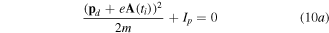


Here, tr is the re-collision time with the parent ion,  is the electron drift momentum, and N is the harmonic order. The solutions for equation (10) define the electron trajectories, known also as quantum orbits. Equation (10b) requires the electron to return to the parent ion—the prerequisite for recombination. Equation (10c) is a statement about the energy conservation when the electron delivers its energy to the emitted harmonic photon. The solution for equation (10a) describes the electron's trajectories during the tunneling process. Although it gives us some limited knowledge about electron dynamics under the potential barrier, this solution requires us to introduce the concept of complex time and complex momentum, for which the physical meaning is hard to interpret.
If we wish to take the analogy between the electron wave-function and the electromagnetic field, the analogous to the electron trajectories are the optic rays. Optic rays are lines which are anywhere perpendicular to the constant phase planes. In most cases, optic rays are just straight lines, but not for example in an inhomogeneous medium. It is worth noting that the classical electron trajectories, derived from the Hamiltonian (3) without a potential, are just straight lines. Now, If we could fabricate a curved waveguide, as in figure 1(a), and probe the electromagnetic wave anywhere at close proximity to the waveguide, we could find the optical rays even in the 'forbidden zone', thus, finding the 'electron trajectories' under the barrier.
3. Simulation
3.1. Methods
To demonstrate the feasibility of our proposed 'optical simulator', we run a finite element numerical simulation (Comsol Multiphysics). Instead of solving the time dependent Schrödinger equation for the electron, we solve the full Helmholtz equation for the curved optical waveguide. To convert back and forth between the atomic physical problem and the curved waveguide problem, we used the dimensionless time and lengths as mentioned above (see figure 1). Our simulation consists of an electromagnetic wave with a carrier frequency  which propagates in a curved step index waveguide, having a core index of refraction
  and an ambient index of refraction
  . The curved waveguide has a width of
  and it follows the curve:

In our simulations we set  , and we varied A and
  . For example, a simulation with the aforementioned parameters, with
  and
and  is equivalent to a particle in a finite square well potential having a width of 4.6 Bohr radius, ionization energy of 20.8 eV, subjected to a laser radiation at 720 nm with intensity of
  . Because of limited computer resources, we break the entire medium into small slices, each slice having a length of
  . We calculated the wave propagation in one slice and used the wave-function at the end boundary as an initial boundary condition for the next slice and so on. To calculate the 'electron trajectories' (optic rays), we first calculated
  which is the analog to the Klein–Gordon probability current
  We next calculated the trajectory direction at each point:
  , and used it to calculate the electron trajectory
  .
.
3.2. Results
Figure 3 shows the normalized  in a logarithmic false color scale. Here we simulate a
  wide, 300 mm long waveguide with core refractive index
  and
and  . The oscillation amplitude is
  . Accordingly, the Keldysh parameter changes from
  (
( at
at  to
to  (
( ) at
) at  , i.e., changes from the 'multi-photn ionization' regime into the 'tunneling ionization' regime. In the figure we indicate the curved waveguide with black dash-dot lines. The adiabatic tunneling exit point (TEP),
  is indicated with the dotted yellow line. Qualitatively, we can see from this figure that each time, near the maximum curvature of the waveguide, radiation is released from the waveguide with an almost point-like radiation source pattern (near the tips of the red arrows). We can see also how these consecutive sources are interfering with each other.
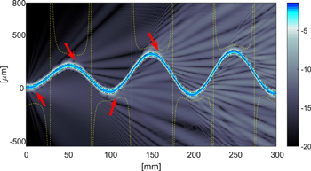
Figure 3. Shows the normalized  in a logarithmic false color scale. The step index waveguide is a
  wide and 300 mm long with core refractive index
  and
and  (black dash-dot lines). The oscillation amplitude (curve given by equation (11)) is
  . It is equivalent to a particle in a finite square well potential having a width of 4.6 Bohr radius, ionization energy of 25.8 eV, subjected to a laser radiation at 720 nm with intensity of
  . The TEP,
  is indicated with the dotted yellow line. The red arrows indicate qualitatively the point-like radiation sources around the maximum curvature.
Download figure:
Standard image High-resolution imageWe want to examine more closely the electron trajectories and compare them to the electron trajectories in the semi-classical model. We focus on ionization points around z = 200 mm where the Keldysh parameter is lower than one. Figure (4) shows long, short and near cut-off trajectories (green, red and yellow solid lines) as well as other representative trajectories (gray solid lines). The dotted pink, red and yellow lines are the corresponding semi-classical trajectories assuming the electron emerges at the adiabatic exit point  with zero velocity (figures 4(a) and (c)) or from the waveguide core (figures 4(b) and (d)). The reason for drawing the two cases is because the three-step-model first assumes that the electron emerges into the continuum at the tunneling exit point with zero velocity (equation (10a)), but equation (10b) assumes that the electron motion starts at r = 0. To extract the resulting electron trajectories (optic rays) from our numerical simulation, we first selected a point, which is far enough from the ionization point. Next, we used the above-mentioned procedure to calculate the trajectories from this point back to the ionization region, and forward to where the electron trajectories collide again with the oscillating waveguide (re-collision). From here on we will refer to the trajectories that we extracted from the numerical simulation as the 'numerical trajectories' (NT); to distinguish them from the semi-classical trajectories (SCT). To compare the NT with the SCT, we first recall that in the transformed coordinates (equation (2a)), the electron trajectories away from any potential, are just straight lines. Therefore, we first find the NT slope at the point far away from the ionization region. We then draw a straight line with the same slope and find the position zi at which this line is tangent to q(t). Finally we shift the line in the
  direction, either to start from the waveguide core (figure 4(b)) or from the TEP (figure 4(a)). The dash-dot purple line in figures 4(c)–(d) is proportional to the second derivative of q(z) (proportional to
  ).
).
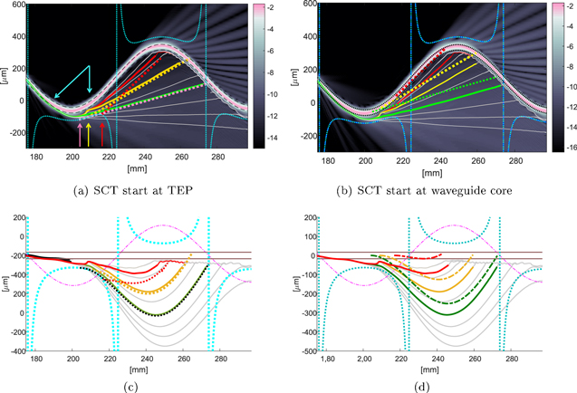
Figure 4. Presents a zoom-in from a simulation with the same conditions as in figure 3 around  Here we show in detail the NTs and the SCTs. The green, red and yellow solid lines are the NTs of long, short and near cut-off trajectories, respectively. The doted lines with the red, yellow and pink, are the corresponding semi-classical trajectories, starting from the TEP (4(a)) or from the waveguide core (4(b)). The trajectories in figures 4(c) and (d) are the same as in figures 4(a) and (b) but translated back to the inertial frame. The waveguide is marked by the two horizontal lines and the dashed-dot purple line is proportional to the second derivative of q(z).
Download figure:
Standard image High-resolution imageAt first glance, the NT look very similar to the SCT, but if we look more closely we can see some differences. The first difference to note is the ionization times. As it is well known in the three-step-model, the different trajectories emerge at the continuum at different times ti. These ti are indicated in figure 4(a) with the red, yellow and pink arrows. The simple-man model gives us no information about the electron trajectories inside the 'forbidden zone' under the barrier. In contrast, from our numerical method we can extract the NT, even in the 'under the barrier zone'. Looking at the NT, we see that all are starting almost at the same point (slanted cyan arrow) and propagating as a bundle until they reach a branching zone (vertical cyan arrow), from which, each trajectory deflects into a different angle. We note also that this branching zone is placed, neither at the TEP, nor at the waveguide edges but placed somewhere in-between.
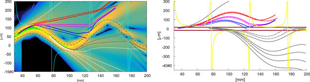
From figure 4 we can see that, in contrast to the semi-classical model, only the long trajectories are really emerging through the TEP (marked by the dotted cyan line) while the short trajectories never really tunnel out. Figure 5 shows the transition from tunnel ionization to above-the-barrier ionization (ABI). The simulation parameters in this case,  and
and  , correspond to an atom with ionization potential
  subjected to laser radiation at central wavelength of 720 nm and intensity of
  . The Keldysh parameters are
  at
at  and
and  at
at  and
and  at
at  where the TEP reach the waveguide edges and we are entering into the ABI. We first look at the tunnel ionization, which occurs around
  . In terms of matching between the semi-classical trajectories and the actual trajectories, it is not much different than the case in figure 4. The slight difference is that here most of the ionized trajectories start deeper from within the waveguide. This difference is even more pronounced at the ionization event near
  and around
  where we reach the ABI threshold, the waves 'spill' out of the waveguide in almost a straight line.
Figure 5. Shows the transition from tunnel ionization to ABI. The simulation parameters in this case,  and
and  , correspond to an atom with ionization potential
  subjected to laser radiation at central wavelength of 720 nm and intensity of
  . The Keldysh parameters are
  at
at  and
and  at
at  and
and  at
at  where the TEP reach the waveguide edges and we are entering into the ABI.
Download figure:
Standard image High-resolution image
4. Conclusion
In summary, we discussed the similarities between the adiabatic tunneling ionization and bending losses in a curved optical waveguide. We show how the problem of an atom in a strong field may translate into the problem of wave propagation in a curved waveguide. Taking this correspondence, we proposed to fabricate a curved waveguide that will simulate the atom in a strong field which allows us to probe the wave-function at any point, including the 'tunneling' region. The results from such a simulator may give answers to many still open questions in strong field physics. We solved numerically the full Helmholtz equation for the electromagnetic wave, propagation through the curved waveguide, and demonstrated the feasibility of such a curved waveguide simulator. Finally, we showed how ray optics may mimic the electron trajectories, including tunneling, free-space propagation and re-collision.
Acknowledgments
GM acknowledges the support of the Israel Science Foundation (404/12) and from the Wolfson Foundation; MK acknowledges the support of the Peter Brojde Center for Innovative Engineering and Computer Science.
Appendix
To allow the interpretation of the proposed optical waveguide simulator, we want to put both the Schrödinger equation and the Schrödinger-like equation from the paraxial approximation, on an equal footing. For that purpose, we put both in a dimensionless form.
We start by writing down the Helmholtz equation:

In the paraxial approximation we assume  , where
  is slowly varying in the z direction. If we differentiate the field twice with respect to z we get:

where  . Since ε is a slowly varying in the z direction, we may neglect
  in equation (13). Substitute (13) back into the Helmholtz equation (12) we get a Schrödinger-like equation:
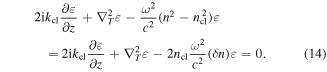
We next change to dimensionless coordinates  and get the dimensionless Schrödinger equation:

Here  .
.
Next we want to put the Schrödinger equation 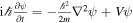 in a dimensionless form as well. We define dimensionless time and lengths
  ,
,  and the Schrödinger equation in this dimensionless coordinates is:

which after rearrangement of terms reduces to the dimensionless form:

Comparing equation (15) with equation (17) we can identify the equivalent quantities: 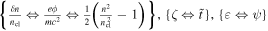 .
.
As a last comment to this appendix, we mention that the scaling given here is not unique. One can use the following additional scaling,  , to keep equation (15) intact. Here, S is a scaling parameter.