


Abstract
Doppler-free optical double-resonance spectroscopy is used to study the  excitation sequence in room-temperature rubidium atoms. This involves a
  electric dipole preparation step followed by the
  electric quadrupole excitation. A detailed experimental and theoretical study of the dependance on the excitation beams polarization from the 420 nm decay fluorescence (
 ) is presented. When a circularly polarized preparation beam is used, it produces a strongly oriented
  intermediate state. In this case a linear quadrupole excitation beam transfers the oriented state to the
  hyperfine states. For linearly polarized preparation and quadrupole excitation beams the spectra of the
  hyperfine lines follow a cosine squared dependence on the angle between the polarization directions. As a consequence, it is shown that the choice of polarization configuration allows direct use of the electric quadrupole transition selection rules to control the populations of the
  hyperfine magnetic sublevels in the absence of external fields. This is achieved by independently enhancing or suppressing either
  or ±2 electric quadrupole transitions.
Export citation and abstract BibTeX RIS
1. Introduction
Optical–optical double-resonance laser spectroscopy is a widely used technique to perform Doppler-free studies of transitions between excited states of atoms [1]. One laser is used to excite ground state atoms into the initial state of the transition, and a second laser produces the desired excitation. When the preparation laser frequency is fixed within the Doppler well of the first transition and the excitation laser is either co- or counterpropagating with the first one, one can obtain velocity-selective spectra [2] with linewidths significantly smaller than the Doppler width of the preparation transition (recent examples are [3–8]). There are many examples of the use of optical-optical spectroscopy to study electric-dipole transitions to excited states in atoms [1] but only recently this technique has been used to perform Doppler-free studies of electric dipole forbidden transitions in room temperature atoms [9, 10].
Many articles develop the theory of coherent mixing for two photon interaction in which one of them corresponds to a dipole forbidden transition (see for example [11]). In this context Miranova et al propose that the polarization state of the light field could be use to control the efficiency of coherent mixing [12].
In this paper we demostrate experimentally that control of polarization states can be used to transfer atoms into specific quantum states. We propose a novel technique that allows the control of selection rules without magnetic field and then production of specific atomic systems via polarization beam configuration. Results for different polarization configurations of the combined preparation and quadrupole excitation lasers are given. Furthermore, it is shown that polarization configuration can be chosen to distinguish between the dynamics of the preparation stage and the selection rules of the electric quadrupole transition. This could be a useful toolbox beyond the dipole approximation, for example in the study of polarization degree in optical transitions as made by Baumgartner et al [13] and in the study of quantum beat spectroscopy made by Bayram et al [14].
A recent article by our research group [9] showed that optical-optical double-resonance spectroscopy can be used to observe the  electric dipole forbidden transition in room temperature rubidium atoms with resolution of the
  hyperfine states. In the present work a detailed investigation of the effect of the light polarization on the relative intensities of the
  electric-dipole forbidden transition is presented. Using linear polarization for both preparation and electric quadrupole beams, with different electric field orientations allow the direct study of the electric quadrupole selection rules over the MF magnetic quantum numbers. With a circularly polarized preparation beam and a linearly polarized electric quadrupole beam, one probes different dynamics of the preparation stage. Experimental spectra for both 85Rb and 87Rb are presented. The experimental data are compared with the results of calculations that consider a
  preparation step that establishes the magnetic sublevel populations of the
  intermediate state, followed by a
  electric quadrupole probe that does not significantly modify the populations of the
  magnetic sublevels. This three step model that includes an electric dipole forbidden transition explicitly takes into account the experimental polarization configurations. Furthermore, the model allows a direct calculation of the relative populations of the hyperfine magnetic sublevels in the
  manifold, and it is shown that these populations can be controlled by the polarization of the electric quadrupole excitation laser.
This paper is structured as follows. Section 2 presents the relevant theory, starting with a discussion over the involved set of rubidium transitions. It also contains a detailed theoretical analysis of the transition matrix elements that occur in each polarization configuration. Furthermore, a discussion of the polarization effects on the production of the magnetic sublevels of the  intermediate state is presented. The role of polarization in the electric quadrupole selection rules leading to production of the different
  hyperfine magnetic sublevels is also shown in detail. The experimental setup is presented in section 3. In section 4 a comparison between the experimental results and the calculations is made. Finally, general conclusions are presented in section 5.
2. Theory
Figure 1 shows the ladder configuration involving the relevant two photon transition followed by a decay straight to the ground state of rubidium. In the experiment a laser in resonance with the  transition at 780 nm (D2 line) is used to prepare atoms in the
  state. In particular, the preparation laser frequency is chosen to excite atoms in the
  hyperfine state, where I is the nuclear spin. A second laser beam at 911 nm is used to produce the
  electric dipole forbidden transition. We detect this excitation channel via 420 nm fluorescence emission for spontaneous decay from
  state into the
  ground state.
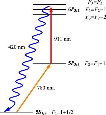
Figure 1. Energy levels of rubidium.
Download figure:
Standard image High-resolution imageThe probability to observe a 420 nm photon resulting from the decay of the  hyperfine states can be written as [9]:
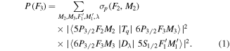
Here  is the population of the
  prepared by the 780 nm laser, Tq is the electric quadrupole transition operator, and Dλ is the
  electric dipole decay operator associated to the light polarization state λ of the 420 nm decay fluorescence. The sum is performed over all projections of total angular momenta of the initial M2 and final M3 states of the non-dipole transition, the angular momenta of the final
  hyperfine states
  , and also over two orthogonal polarization directions λ. The value of the total angular momentum of the intermediate state F2 corresponds to the
  cyclic transition of the D2 preparation step. In this expression it is assumed that the electric-dipole coupling of the first step is much stronger than the electric quadrupole excitation. Therefore, the first step determines the populations of the M2 magnetic sublevels of the
  state, which are then weakly coupled to the
  state by the electric quadrupole operator.
Equation (1) shows how the light polarization can be used to modify the relative intensities of the blue fluorescence that results from the decay of the hyperfine manifold  . On the one hand, the polarization of the 780 nm preparation laser allows control of the relative M2 populations of the
  intermediate state. A linearly polarized
  electric-dipole excitation produces a
  aligned state, while a circularly polarized light produces an oriented state [15]. On the other hand, a linearly polarized electric quadrupole coupling beam will transfer the
  orientation or alignment into the
  hyperfine states. The relative populations of these hyperfine states can be obtained by direct summation of the first two terms in equation (1) over the magnetic quantum numbers M2. The anisotropy in these populations translates into different relative intensities of the 420 nm fluorescence lines.
For the implementation of the three step model it is necessary to define the coordinate system for the two polarization configurations studied in this work. In figure 2 both laser beams are counter propagating, while the detection direction is orthogonal to laser propagation. These directions define the horizontal plane. The polarization state of the preparation laser determines the quantization axis for each polarization configuration. For a linearly polarized preparation beam the quantization axis is chosen parallel to its electric field along the z vertical direction, then the propagation direction becomes the x axis and the electric field vector of the electric quadrupole laser lies on the yz plane, making an angle θ with respect to the vertical axis. In the other polarization configuration, in which the preparation laser is circularly polarized and the electric quadrupole laser is linearly polarized, the propagation axis is now the quantization axis (defined as z axis). This time, the electric quadrupole excitation laser is chosen to have its electric field vector  parallel to the vertical direction, which is now the x axis.
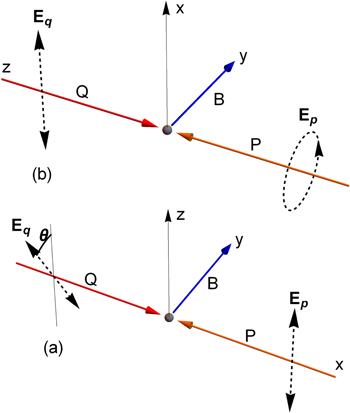
Figure 2. Geometry used in the calculation. Colinear preparation (P) and electric quadrupole (Q) beams define the propagation direction. The 420 nm fluorescence is detected along the y axis. (a) Linear–linear configuration. The electric field vector of the preparation beam defines the z-axis. The electric field vector of the quadrupole beam makes an angle theta with respect to the z-axis. (b) Circular–linear configuration. The propagation direction of the preparation beam now defines the z-axis.
Download figure:
Standard image High-resolution image2.1. Dipole transitions
The three step model (equation (1)) includes two electric dipole transitions. The first one is the  excitation that prepares the initial states of the electric quadrupole transitions
  . After the interaction with the electric quadrupole laser some of the atoms are excited into the
  manifold. There is a finite probability for these excited atoms to decay via the
  electric dipole transition.
2.1.1. Preparation step
First we show that our choice of the preparation step frequency also fixes the value of the  hyperfine state in equation (1). In principle one can excite, for well defined values of the axial atom velocity, each of the
  , F1 and
  transitions. However, the
  and F hyperfine states have a finite probability of decaying into the
  ground state (dark state) that can no longer interact with the preparation laser. Atoms in these
  intermediate states are therefore pumped out of the preparation step. One therefore expects electric quadrupole spectra that are dominated by the
  cyclic transition in the preparation step. The calculation shows that there is only one electric quadrupole transition that involves a
  hyperfine state outside of this cyclic transition. Optical pumping into the dark state significantly reduces its intensity, and it will not be included in the model.
The temporal evolution of the relative populations of the  magnetic states is calculated using the Einstein rate equation approximation. The assumption is made that initially the
  magnetic sublevels are statistically distributed. The system of equations is solved using the Euler method. A time averaging on the instant populations
  states is performed to determine the effective population available for the electric quadrupole transition. The integration time is the transit time Ttrans of the atoms across the preparation beam [16]. For our experimental conditions we estimate
  .
.
For a linearly polarized preparation beam the temporal evolution of the  magnetic sublevels M2 of 85Rb is presented in figure 3(a). In this case the selection rule
  prevents excitation into the
  sublevels. The integrated populations are given in figure 3(b), which shows that the system accumulates the maximum population in the
  state. As expected for lineraly polarized light, the populations of the negative M2 levels are equal to those of the positive M2 levels, which means that one ends up with an aligned atomic ensemble [15].

Figure 3. Temporal evolution (upper panels) and average populations (lower panels) for the  states in
  . The left panels correspond to preparation with a linearly polarized laser. In this case the evolution of the
  states is identical to that of the
  states. The right panels are for a circularly polarized preparation laser.
Download figure:
Standard image High-resolution imageFor the case of a circularly polarized preparation laser. the calculation was performed under similar conditions, but now the selection rule is  . The temporal evolution is shown in figure 3(c) and the population time average is shown in figure 3(d). In this case the population accumulates in the extreme
  magnetic state, resulting in a strongly oriented system [15].
Qualitatively similar time evolution curves and relative population distributions are found for different values of the preparation laser intensity I780. The time to achieve the steady state is reduced for higher values of I780 and the corresponding asymptotic population values are larger. However, it is interesting that the ratios  remain almost constant for I780 below the saturation intensity. Equivalent results were obtained for 87Rb.
2.1.2. Decay process
Decay from the  is the other electric dipole process in the three step model. In our geometry the blue fluorescence is always detected along the y axis. Therefore, the electric field vector for the 420 nm photons is in the zx plane. In our experiment we do not select the final hyperfine state of the decay nor the polarization state of the 420 nm photon, the contribution of this third step is the incoherent sum for the polarization states
  , x given by
This becomes the third factor in equation (1), and is the same for the two polarization configurations studied in this work.
2.2. The electric quadrupole transition
2.2.1. Linear–linear configuration
With the geometry described in figure 2 the electric field  can be separated in two components, one of them
  is parallel to the quantization axis with an amplitude
  and the other component,
  is perpendicular with an amplitude
  . Since the tensor operator for an electric quadrupole transition is
  , we can write each component of the transition matrix element for the quadrupole excitation as
where the Wigner–Eckart theorem is used to separate the dynamical part from the geometric part. Two different selection rules for the magnetic quantum numbers result from these equations. They are  for parallel linear polarizations and
  for the perpendicular case.
The square of the complete quadrupole transition matrix element gives the probability for the second step in the process. Taking into account that the contributions have different selection rules, the second step probability can be written as
where  denotes the dependence of the transition in the angle
  between the linear polarized electric fields E1 and E2.
When one substitutes the corresponding expressions for time average population  given in figure 3(b), the quadrupole electric probability in equation (5), and the decay probability in equation (2) into equation (1) and after performing the sums over M2, M3 ,
  and
and  , one obtains a function that describes the angular distribution of the probability to observe a 420 nm photon for each
  hyperfine state,

where the coefficients P∥ and P⊥ are given by
2.2.2. Circular–linear configuration
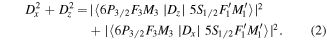
When the circular preparation beam defines the quantization axis z as the propagation direction, the quadrupole electric field vector  lies on the xy plane. In this case, the transition probability does not depend on the angle θ, therefore for calculation convenience
  is taken parallel to the vertical direction, i.e.
  in figure 2. Then the electric quadrupole transition matrix element is
The transition probability for quadrupole transition is the square of equation (9), its value is used to calculate the second term in expression equation (1) for the circular linear polarization case.
3. Experimental setup
Details of the experimental setup were presented in [9]. Here only the modifications made for the polarization studies (see figure 4) are presented. The 780 nm preparation beam is taken from an external cavity diode laser (ECDL). The 911 nm quadrupole excitation beam is now a commercial CW titanium-sapphire laser (Ti:Sapphire, M Squared Lasers). The polarization states of two beams are prepared before they counterprogate along a rubidium cell at room temperature. A quarter wave plate is added for the experiments with a circularly polarized preparation beam. The degree of polarization of the preparation beam was measured both with and without the quarter-wave plate. Without the quarter-wave plate a  linear polarization was obtained and with the quarter-wave plate we obtained
  circularly polarized light. Finally, the use of a half-wave plate allows to rotate the linear polarization of the 911 nm electric quadrupole beam with polarization degree of
  , limited by the optical setup.

Figure 4. Experimental setup for polarized Doppler-free double resonance spectroscopy. ECDL: external cavity diode laser; TiSa: titanium-sapphire laser; Q: 780 nm quarter wave plate; H: 911 nm half wave plate; PMT: photomultiplier tube; M: mirror, L: lens system; F: 420 nm interference filter, C: chopper, PSD: phase sensitive detector, PC: computer.
Download figure:
Standard image High-resolution imagePolarization spectroscopy is used to lock the frequency of the 780 nm preparation laser to the Doppler free  cyclic transition (F = 2 in 87Rb or F = 3 in 85Rb) [16–18]. An optical system with two lenses and a 20 nm bandpass filter is used to collect the 420 nm blue fluorescence into the photomultiplier tube. A phase-sensitive detection system is used to obtain the
  electric quadrupole excitation spectra. The initial tuning of the 911 nm laser is achieved with a wavemeter with a 0.050 nm resolution. A Fabry–Perot interferometer is used to monitor the single-mode operation of the 911 nm laser, and it also provides a coarse frequency scale, but the final callibration is made by comparing the spectra to the known hyperfine splittings of the
  state [19].
For the 911 nm beam a power of 50 mW was used, which results in an average intensity of 6.2 kW m−2. For the 780 nm preparation beam  of power were used with an average intensity of 10.7 W m−2, below the 16.46 W m−2 saturation intensity for the D2 transition [20].
The two polarization configurations of interest were already discussed in section 2. In the first one a linearly polarized light is used for both the  preparation step and the
  quadrupole excitation. The intensity of the
  hyperfine fluorescence lines were measured as function of angle θ between polarization vectors giving angular distribution curves for each hyperfine state. Two measurement methods for each angle θ were used to construct the angular distribution curves. In one, full spectra were recorded and the line intensities were obtained for each spectrum. The overall intensity and the relative hyperfine intensities of these spectra depend on the stability of the preparation laser. In the course of the measurements both frequency and intensity were found to fluctuate. Thus, for each angle several individual spectra were obtained to average out these fluctuations. This procedure magnified systematic effects that resulted from drifts in the laser intensity and frequency. In the second procedure shorter scans across individual lines were recorded and the line intensities were directly read from the peak heights of these short scans. Direct comparison of these two methods results in angular distributions that agree with each other, but with less scatter and smaller error bars in the data obtained with the shorter scans.
The relatively low polarization of the quadrupole excitation light imposes a correction in equation (6) that can be included by considering an extra contribution for two orthogonal components electric field vectors,  making an angle θ with respect to the quantization axis, and
  that now makes an angle
  with respect to the quantization axis. The separate contributions to the line intensities are:
where  for perfect linear polarization is given by equation (6). The resulting angular distribution can be expressed in terms of the degree of polarization

In the second polarization configuration a circularly polarized preparation beam and a linearly polarized quadrupole beam are used. The model predicts that in this case there should be no effect in the relative line intensity if the linear polarization direction of the 911 nm laser is rotated. A quick test of this prediction was made, and no angular dependence on θ was found in the circular–linear case.
4. Results and discussion
4.1. Linear–linear polarization
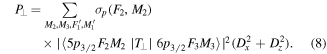
Figure 5 shows typical spectra for 85Rb obtained whith linearly polarized lasers when the electric fields are parallel (bottom) and perpendicular (top). Each of these two spectra isolate the corresponding contribution of P∥ and P⊥ in equation (6). These spectra independently probe the  and
and  electric quadrupole selection rules. The calculated hyperfine intensities are also indicated by vertical bars in this figure. In these spectra a constant background was subtracted from the experimental data. The calculated values include the effect of a partially polarized 911 nm beam, equation (10). Both spectra show the three hyperfine components
  , 3 and 4, and a weaker peak that results from the velocity selected
  excitation sequence [9]. This is the only velocity selective excitation with a significant electric quadrupole transition probability and it was not included in the calculation. The results of Voigt profiles to each line, all with the same widths (11.5 MHz FWHM) are also indicated. The two extreme cases of the linear–linear configurations display rather different relative hyperfine intensities, all in good agreement with the model. For parallel polarizations the maximum occurs for
  , with almost equal contributions from the
  and
and  lines. In the case of perpendicular polarizations the maximum corresponds to
  , with a very small contribution from
  .
.
Figure 5. Fluorescence emission spectra of 85Rb for linear polarization of both preparation and electric quadrupole excitation lasers. The numbers give the position of the three  hyperfine fluorescence lines. The vertical bars give the position and calculated relative intensity of each hyperfine fluorescence line. The parenthesis indicates the position of the
  velocity selected line which is not included in the calculation.
Download figure:
Standard image High-resolution imageThe angular distribution of the decay fluorescence was measured for each  hyperfine line. The results are shown in figure 6. The solid symbols give the intensities obtained from averages over several full spectra recorded at each value of θ. The open symbols are the result of quick scans of separate hyperfine lines. The two measurement methods agree with each other within the experimental error, that is given by statistical fluctuations only. The continuous lines are the result of the calculation. They include the effect of a partially polarized quadrupole beam. To compare experiment and theory in a single plot, a constant background and an overall normalization factor are needed. The degree of polarization of the 911 nm was used as a third parameter in the fit. These three parameters were optimized, in a least squares sense, simultaneously for the three hyperfine peaks. The theoretical curves in figure 6 were obtained for a polarization
  , which is within the measured value of
  . The fitted constant background was consistent with the one obtained for each individual spectrum. There is very good agreement between experiment and theory. The cosine squared angular distribution is confirmed for all three lines. The F = 4 hyperfine line has a minimum at
  and a maximum at 90°. The opposite behavior is found for the F = 3 and F = 2 hyperfine lines. Also, the largest changes occur for F = 4. The F = 2 lines is always below the other two lines, but at 0° its intensity is close to that of the F = 4 line.

Figure 6. Dependence of the 85Rb fluorescence intensity on the relative direction of the linear polarization of the electric quadrupole laser with respect to the linear polarization of the preparation laser. The continuous lines give the calculated angular distributions, corrected for the degree of polarization of the 911 light. For the meaning of the symbols, the normalization procedure and the inclusion of the partial polarization effect see the text.
Download figure:
Standard image High-resolution imageFor 87Rb a comparison between parallel and perpendicular spectra, and also between experiment and theory, is presented in figure 7. These spectra are similar to the ones found for 85Rb (figure 5). For this isotope we did not perform a full angular distribution measurement, but the agreement between experiment and theory for the parallel and perpendicular cases, and the results for 85Rb, give us confidence in the validity of the three step model.

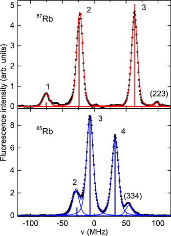
Figure 7. Fluorescence emission spectra of 87Rb for linear polarization of both preparation and electric quadrupole excitation lasers. The numbers give the position of the three  hyperfine fluorescence lines. The vertical bars give the position and calculated relative intensity of each hyperfine fluorescence line. The parenthesis indicates the position of the
  velocity selected line which is not included in the calculation.
Download figure:
Standard image High-resolution imageA comparison between experiment and theory for the relative intensity of the hyperfine fluorescence lines is also made in table 1, where we present numerical results normalized so that the sum of the three intensities is equal to one. The first line for each isotope gives the theoretical values obtained for a polarization  , while the second line gives values corrected for a polarization
  . The main effect of a partially polarized electric quadrupole beam is to reduce the contrast between the different fluorescence lines. The experimental numbers are the result of the average over the recorded spectra. Once again, there is very good agreement between and experiment.
Table 1. Relative intensities of hyperfine lines.
| 87Rb | Parallel | Perpendicular | ||||
|---|---|---|---|---|---|---|
| F3 | 1 | 2 | 3 | 1 | 2 | 3 |
Calculated ( ) ) |
0.14 | 0.61 | 0.25 | 0.01 | 0.26 | 0.72 |
Calculated ( ) ) |
0.13 | 0.59 | 0.28 | 0.03 | 0.30 | 0.67 |
| Experiment | 0.13(2) | 0.59(8) | 0.28(4) | 0.045(6) | 0.32(4) | 0.63(5) |
| 85Rb | Parallel | Perpendicular | ||||
| F3 | 2 | 3 | 4 | 2 | 3 | 4 |
Calculated ( ) ) |
0.22 | 0.60 | 0.18 | 0.03 | 0.34 | 0.63 |
Calculated ( ) ) |
0.18 | 0.55 | 0.27 | 0.07 | 0.37 | 0.56 |
| Experiment | 0.20(2) | 0.57(4) | 0.23(3) | 0.07(1) | 0.36(2) | 0.57(4) |
The confidence on the model is used to infer the relative population for each of the magnetic sublevels in the upper states  . This population is calculated using the excitation terms in equation (1), with the sum performed over the M2 quatum numbers. Figure 8 shows the calculated populations for each of the magnetic sublevels of the
  , 3 and 4 hyperfine states of 85Rb. They correspond to the linear–linear excitation configuration. The parallel configuration is contrasted with perpendicular configuration for each F3 state. For parallel configuration, in which the
  selection rule the
  state has the greatest population. For perpendicular configuration the selection rule is
  and now the
  state has the greatest population. All the F3 states show distributions that are symmetrical with respect to
  , something characteristic of aligned states. However, only for the
  state the
  has the largest population. For
  . The maxima are at
  and for F = 4 they are at
  . This is definitely a population distribution characteristic of an electric quadrupole transition. These population distributions reflect the interplay between the
  population distributions produced by the preparation laser shown in figure 3 and the geometric matrix elements of the electric quadrupole transition, which are determined by the electric quadrupole selection rules.

Figure 8. Relative population in  states for 85Rb hyperfine states for the linear–linear polarization configuration. The left column shows the populations for parallel polarizations (here the selection rule
  applies). The right column gives the populations for perpendicular polarizations, when the
  selection rule applies. Note the differences in the ordinate scales.
Download figure:
Standard image High-resolution image4.2. Circular–linear polarization
The relative intensities of the  hyperfine fluorescence lines are also different for the configuration in which the 780 nm preparation laser is circularly polarized and the 911 nm electric quadrupole beam is linearly polarized. In this case the differences occur because of the different populations of the M2 magnetic sublevels of the
  intermediate state. Circularly polarized light produces a strongly oriented atomic state, with most of the population in either
  state for right circularly polarized light, and
  for left circularly polarized beam. As shown in figure 3(d). Figure 9 shows typical spectra for each isotope along with the calculated intensities. In this case one does not expect any effect because of the polarization of the quadrupole beam, therefore no corrections were included in the calculation. There is, again, very good agreement between experiment and theory. For both isotopes the two strongest peaks have comparable intensities. For 85Rb both theory and experiment agree on the F = 3 peak being larger compared to F = 4. However, theory underestimates the intensity of the F = 2 peak. For 87Rb the experimental spectra give the same intensities for both F = 2 and F = 3. The calculation gives F = 3 a slightly larger contribution. As for the other isotope, the model underestimates the intensity of the F = 1 peak. Both spectra show the presence of the
  velocity selected peak.
Figure 9. Fluorescence emission spectra for the circularly polarized preparation laser and a linearly polarized electric quadrupole excitation laser. The vertical bars give the position and calculated relative intensity of each hyperfine fluorescence line. The parenthesis indicates the position of the  velocity selected line which is not included in the calculation.
Download figure:
Standard image High-resolution image
5. Conclusions
We presented theoretical and experimental results showing that light polarization plays a major role in the Doppler-free study of the  electric quadrupole transition. Our three step model is crucial to interpret the experimental results. It shows that the magnetic state populations of the intermediate state
  are controlled by the polarization of the preparation laser. Linear polarization produces an aligned state with maximum population for
  . Circularly polarized light produces an oriented state with almost all the population in the stretched state
  . In the second step the use of linear polarization for the electric quadrupole laser transfers the orientation/alignment of the
  state into the
  hyperfine states. The signature of the orientation/alignment is found in the relative line intensities of the decay fluorescence line of each of the hyperfine
  states. For the linear–linear polarization configuration, the experimental data confirm a cosine squared dependence of the hyperfine line intensities as a function of the angle θ between the polarization directions. The calculation accurately reproduces the behavior of the angular distribution curves. Particularly interesting results occur for the extreme cases
  and
and  because in the first case the electric quadrupole selection rules
  is the only one that applies, and when the polarizations are perpendicular, in the second case, the selection rule is
  . This is cannot be achieved with an electric dipole transition. Hence, the choice of light polarization in an electric quadrupole transition allows independent control of the
  or ±2 transitions. Thus polarization control of electric quadrupole transitions can potentially become a very useful tool in the manipulation of quantum states of atoms. Even though the results presented here apply to thermal rubidium atoms, both experimental and theoretical methods can be applied to other alkali atoms [9, 21]. Combining state of the art diode lasers with sub-megahertz emission widths [22, 23] and the three-step model one should be able to interpret forbidden spectra for potassium, which has 4p and 5p hyperfine structure with separations comparable to the natural width.
Acknowledgments
We thank J Rangel for his help in the construction of the diode laser. This work was supported by DGAPA-UNAM, México, under projects PAPIIT Nos. IN116309, IN110812, and IA101012, by CONACyT, México, under Basic Research project No. 44986 and National Laboratory project LN260704.