

Abstract
A typical undergraduate course in mechanics does not cover the fascinating and important gravity-assist manoeuvre that allows satellites or other spacecrafts to navigate through our solar system on efficient and desired paths. Instead, it usually remains a mystery to students how energy is conserved when a spacecraft gains speed as it flies past a planet. Indeed, one might be led to believe that the curved path of the planet is the root cause for the gain in speed, requiring consideration of gravity-assist within the framework of the restricted three-body problem. This contribution will emphasize that this extension is not required to explain the gain in kinetic energy. Instead, a simple, scaffolded analysis of the planet-satellite system alone, using elementary physics, two reference frames and analytical methods, provides a sufficient explanation. Our simplified analysis is successfully validated against mission data from Voyager 2's gravity-assist manoeuvre around Jupiter.
Export citation and abstract BibTeX RIS

Original content from this work may be used under the terms of the Creative Commons Attribution 4.0 licence. Any further distribution of this work must maintain attribution to the author(s) and the title of the work, journal citation and DOI.
1. Introduction
Most undergraduate mechanics courses for physics majors cover Kepler's problem, meaning the motion of two celestial bodies about their common center-of-mass [1, 2]. The emphasis lies on bound states in the Sun-planet system, comprised of elliptical, planetary orbits that include circular orbits as special cases. In contrast, the importance of unbound states, characterized by hyperbolic or parabolic orbits, is hardly discussed or not discussed at all, other than being two additional features of conic sections and solutions of the Kepler problem for zero and positive total energy of the planet, respectively [1–4].
Instead, such unbound (free) states of motion are usually discussed in the context of Rutherford scattering, the elastic scattering of charged particles by the Coulomb interaction [5]. Conveniently, the scattering of a charged particle by another particle of opposite charge can be easily mapped onto the gravitational scattering of a satellite or other spacecraft by a planet [5, 6] since both the gravitational and the electrostatic force scale with the inverse of the square of the displacement between the objects.
In celestial mechanics, scattering plays a crucial role in the gravity-assist manoeuvre, in which a satellite changes direction and gains speed in the Sun's frame of reference as it passes through the gravitational field of a planet [6–14]. These scattering events can be used in a controlled, optimized fashion to put satellites on new trajectories that minimize the travel time for a rendezvous with the next planet or other celestial body [10, 12, 14].
Since all celestial bodies move in the Sun's frame of reference (which is nearly identical to the center-of-mass (CM) frame of reference of the entire solar system), the study of gravity-assist manoeuvres and the corresponding optimization of satellite trajectories that connect adjacent planets or celestial bodies are inherently complex problems. In turn, this complexity obscures the underlying principles behind the gravity-assist manoeuvre, leaving most undergraduate students wondering how a satellite can gain speed, and hence kinetic energy, by passing a planet. One may easily look for the root cause for this apparent violation in energy conservation in the curved orbit of the planet. This would require an analysis of the motion within the Sun-planet-satellite system, accurately described by the so-called restricted three-body problem [15, 16]. Here, the Sun and the planet move on their respective circular or near-circular orbits about their common center-of-mass while the much lighter satellite of negligible mass moves within this system. By switching to a rotating reference frame in which the Sun and the planet are stationary, the governing equations for the satellite can be derived in a straightforward manner and simulated numerically [8, 15, 16]. This also includes the study of Lagrange points. Moreover, the three-body system can easily be extended to include other planets, providing a very comprehensive picture of the motion of the satellite within the solar system.
The fundamental concepts of the gravity-assist manoeuvre, however, are much simpler and, of course, known to generations of physicists. It does not require the introduction of the three-body problem. Instead, a simple analysis of the satellite dynamics in two different frames of reference, namely the Sun's and the planet's, reveals how the satellite gains speed [7, 9, 17–21]. Arguably, Broucke's contribution [7] represents a comprehensive treatment of the gravity-assist manoeuvre, yet the analyses within that paper remain outside the comprehension of most junior undergraduate students. Complex treatments that exceed junior undergraduate levels can also be found in the relativistic formulation of Cacioppo et al [17] and Dykla et al [19], the Lagrangian approach that Epstein takes in [20], or Grushevskii's work [9], which starts at the outset with (Rutherford) scattering. At the opposite end of the spectrum, Cook [18] demonstrates in very few steps how the momentum of a satellite changes during gravity assist, using an elementary analysis of momentum balance but without an explicit transformation between coordinate systems. Van Allen's elegant tutorial paper [21] is the closest in scope to our contribution. However, it focuses on changes in energy, not speed, which gives the contribution a slightly different angle. In addition, it does not consider limiting cases of the gain in speed as we do further below in this manuscript.
In contrast, our contribution aims to convey the core principles of gravity assist, also known as swing-by or sling-shot manoeuvre, to any junior undergraduate students of physics and astronomy, especially first-year students, using simple vector algebra. At the same time, it offers guidance to physics and astronomy instructors concerning the teaching of gravity assist. Step by step, we delve deeper into the theory so that both students with no knowledge of (Rutherford) scattering and those with knowledge of scattering benefit from the reasoning presented herein.
In a scaffolded approach, we begin in the next section with a very simple and specific scenario of a satellite being deflected by a planet by 90° towards the forward direction. Subsequently, in section 2.2 we loosen the constraints of the motion and include arbitrary outgoing angles, and even consider arbitrary incoming and outgoing angles in section 2.3. All this can be done without a consideration of the specific interaction, i.e. the inverse-square law of gravitation, between the satellite and the planet but rather via conservation of energy and angular momentum in the planet's frame of reference, and a subsequent transformation into the Sun's frame of reference. This makes the study accessible even to first-year students of physics or mechanics.
In section 3, the analysis becomes more detailed in that the specifics of gravitational scattering are incorporated, yielding a general expression for the change in speed of the satellite in the Sun's frame of reference. In section 4, we validate our simplified treatment against trajectory data of Voyager 2's gravity-assist manoeuvre around Jupiter, demonstrating impressive agreement. Section 5 then provides a brief insight into a more general treatment of the satellite dynamics within the restricted three-body problem, followed by a conclusion.
2. The simplest model of gravity-assist
At the heart of the gravity-assist manoeuvre lies the analysis of the scattering of a light-weight spacecraft 'satellite' 1 as it flies past a massive planet, viewed in two different frames of reference: (i) the planet's frame of reference (figure 1) and (ii) the Sun's frame of reference (figure 2), also referred to as the heliocentric frame of reference. For case (ii), it can be assumed that the swing-by occurs fast enough so that we can consider the trajectory of the planet as being a straight line during this event.

Figure 1. Schematic of a gravity-assist manoeuvre of a satellite with mass m in the frame of reference of a planet with mass M (m ≪ M). In this scenario, the satellite is moving initially in the outward radial direction with respect to the Sun which is located far away along the negative y-axis, being turned by 90° before leaving the gravitational field of the planet again. During this manoeuvre, the planet is assumed to move in the positive x-direction in the Sun's frame of reference.
Download figure:
Standard image High-resolution image
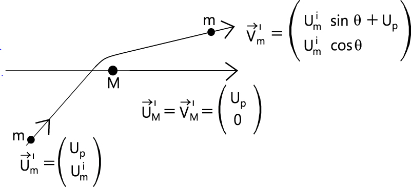
Figure 2. The gravity-assist manoeuvre in figure 1, viewed in the Sun's frame of reference (denoted by 'prime' notation). It is assumed that the manoeuvre takes place sufficiently fast so that the trajectory of the planet can be approximated by straight-line motion during this event.
Download figure:
Standard image High-resolution image2.1. Scattering in the forward direction (+90°)
Specifically, let us consider a satellite of mass m as it changes its direction of motion by 90° while it flies by a planet of mass M, located at the origin, with m ≪ M. In particular, the satellite approaches the planet in an outward direction relative to the Sun, with the Sun placed at a distance dp from the planet and located at (0, −dp ), see figure 1. It is then scattered and leaves the planet's sphere of influence in a forward direction, moving in the same (tangential) direction relative to the Sun as the planet. To first order, this direction is (nearly) perpendicular to the radial direction, if the planet moves on a (nearly) circular orbit.
In general, it will be challenging to realize precisely a 90° manoeuvre. After all, the scattering angle will depend on the exact parameters of the incoming trajectory of the satellite (see section 3). However, this special example is motivated by the gravity-assist manoeuvres of both Voyager 1 and Voyager 2 in the gravitational field of Jupiter where the scattering angle was approx. 90° and approx. 80°, respectively [22]. We will return to the case of Voyager 2 in section 4.
First, we study this scenario in the frame of reference of the planet which, under the assumption m ≪ M, is a very good approximation of the CM frame of the planet-satellite system. Defining a planar, Cartesian coordinate system as in figure 1, and denoting the velocity of the satellite and planet before the scattering event by  and
and  , respectively, and the velocity of the satellite and planet after the scattering event by
  and
and  , respectively, we find
2
:
, respectively, we find
2
:


where  . In other words, the speed of the satellite well before and well after the scattering event is the same since the total energy of the satellite in the planet's frame of reference is conserved which, at large displacement from the planet where the gravitational field of the planet is vanishingly small, equals its kinetic energy,
  .
.
Immediately, the question of conservation of momentum arises. How can it be preserved if the satellite changes direction but not the planet which remains at rest? A rigorous treatment would consider the event in the planet-satellite CM system (denoted by 'double prime') in which the velocity of the satellite and planet well before and after the manoeuvre read:


Here,  and
and  hold exactly so that the total momentum of the system equals zero before and after the gravity-assist manoeuvre while the total kinetic energy of the system remains conserved also. We see that under the assumption of a very light satellite in the gravitational field of a much heavier planet, m/M ≈ 0 holds and we recover the above relations (1)–(4) in the reference frame of the planet. In other words, the reference frame of the planet is a very good approximation of the CM system with respect to the conservation of energy of the satellite but not with respect to its momentum. However, we will focus on kinetic energy and speed in this paper and, hence, the reference frame of the planet suffices for our analysis.
While the gravity-assist manoeuvre appears trivial in the reference frame of the planet, the situation looks quite different in the reference frame of the Sun, relative to which we describe the positions of celestial bodies in our solar system. Since a planet such as Jupiter does not move far along its curved trajectory during a gravity-assist manoeuvre, which takes place over just a few (Earth) days, we approximate the transformation from the reference frame of the planet to that of the Sun during the gravity-assist event by a simple Galilean transformation, given here by a boost along the positive x-axis. More precisely, we add a velocity

to the velocities of the satellite and the planet in the reference frame of the planet, which simulates a satellite that is being scattered in the forward direction with respect to the planet's motion in the Sun's frame of reference (see figure 2). This results in the following description of the event in the Sun's frame of reference (denoted by 'prime'):


This time, the satellite does change its speed overall, according to:

Let us consider three distinct scenarios, namely
- (i)
 : the satellite approaches the planet with a relative velocity that has the same magnitude as the velocity with which the planet travels relative to the Sun.
 - (ii): the satellite approaches the planet with a relative velocity that is much larger than the velocity with which the planet travels relative to the Sun.
- (iii): the satellite approaches the planet with a relative velocity that is much smaller than the velocity with which the planet travels relative to the Sun.


From equation (14), we obtain
- (i): ,
- (ii): ,
- (iii): ,


where we Taylor-expanded equation (14) to linear order for cases (ii) and (iii). (Here, the 'Big O' notation means that the error in case (ii) is bounded by  for some constant H as
  , which becomes arbitrarily small as um
i
grows while up
remains fixed. The error in case (iii) needs to be interpreted accordingly.) We find that the satellite gains speed in all three scenarios as it is being scattered in the forward direction but this gain is bounded by up
. In other words, the satellite cannot gain more speed than the speed with which the planet moves around the Sun at the moment the gravity-assist manoeuvre takes place. Importantly, the specific nature of the interaction between the satellite and the planet, i.e. gravity, has no bearing on the findings. We simply assume it is an attractive rather than a repulsive force but even this assumption could be relaxed.
, which becomes arbitrarily small as um
i
grows while up
remains fixed. The error in case (iii) needs to be interpreted accordingly.) We find that the satellite gains speed in all three scenarios as it is being scattered in the forward direction but this gain is bounded by up
. In other words, the satellite cannot gain more speed than the speed with which the planet moves around the Sun at the moment the gravity-assist manoeuvre takes place. Importantly, the specific nature of the interaction between the satellite and the planet, i.e. gravity, has no bearing on the findings. We simply assume it is an attractive rather than a repulsive force but even this assumption could be relaxed.
2.2. Scattering by an arbitrary angle
Next, we consider the scattering of a satellite by an arbitrary angle θ, as measured from the positive, vertical axis and in the clockwise direction (see figure 3).

Figure 3. Gravity-assist manoeuvre in the planet's frame of reference for the same angle of approach as in figure 1 but for an arbitrary outgoing angle θ.
Download figure:
Standard image High-resolution imageIn the planet's frame of reference, the formulation is now generalized to read


Note that the kinetic energy of the satellite is again conserved. Moving to the Sun's frame of reference, this becomes (see figure 4)


Accordingly, the change in speed for the three different scenarios (i)–(iii) above now reads more universally
- (i): (exact result),
- (ii): (approximation to linear order),
- (iii): (approximation to linear order).


We observe that the satellite gains speed when it is being scattered (at least partially) in the forward direction (0 < θ < 180°) and it loses speed when it is being scattered (at least partially) in the backward direction (−180° < θ < 0) for which it would have to fly around on the other side of the planet. Again, this fundamental result does not depend on the specific interaction between the satellite and the planet. And again, in all three cases the gain in speed is bounded by up .

Figure 4. The gravity-assist manoeuvre in figure 3, viewed in the Sun's frame of reference.
Download figure:
Standard image High-resolution imageWe learn that if an outward moving satellite is supposed to gain speed as it flies by a planet, it needs to be accelerated in the direction in which the planet moves around the Sun at that moment in time. The above analysis is very accurate if (a) m ≪ M and (b) the planet does not move far along its trajectory around the Sun while the satellite passes it so that straight-line motion is a good approximation for the planet's orbit.
2.3. Scattering for arbitrary incoming and outgoing directions
Finally, let us study the case when the satellite approaches the planet at an angle δ (again relative to the positive y-axis and in the clockwise direction), leaving it under an angle θ. The respective velocities in the Sun's frame of reference read

Accordingly, the change in speed becomes
which is positive whenever  or, in other words, whenever the satellite is scattered by the planet in a (more) forward-pointing direction, i.e. the up
-component of the velocity of the satellite increases. Note that this includes cases of (i) negative δ and θ, (ii) negative δ but positive θ, and (iii) positive δ and θ. Again, this fundamental result is independent of the exact nature of the interaction between the satellite and the planet, meaning which precise force law applies.
or, in other words, whenever the satellite is scattered by the planet in a (more) forward-pointing direction, i.e. the up
-component of the velocity of the satellite increases. Note that this includes cases of (i) negative δ and θ, (ii) negative δ but positive θ, and (iii) positive δ and θ. Again, this fundamental result is independent of the exact nature of the interaction between the satellite and the planet, meaning which precise force law applies.
3. Incorporating scattering explicitly
The last step in our exploration of gravity-assist is to incorporate the exact nature of the interaction between the planet and the satellite, namely, the inverse-square law of gravitation. In principle, this allows us to relate the incoming angle δ and the outgoing angle θ in the planet's frame of reference. However, we will be using a slightly different notation in what follows, focusing on forward scattering in which the satellite gains speed.
Figure 5 shows the scenario in the planet's frame of reference in which an incoming satellite moves partially around the 'back' of the planet while it is being scattered towards the forward direction (positive x-axis).

Figure 5. Gravitational scattering of a satellite of mass m in the reference frame of the planet with mass M. The scattering event is uniquely described by the incoming angle β, the speed of approach um
i
, the impact parameter d, and the mass M, which determine the scattering angle γ and, hence, the outgoing angle β + γ. Note that both the kinetic energy,  , and the angular momentum,
  , of the satellite are conserved during this event.
Download figure:
Standard image High-resolution imageDuring this manoeuvre, the planet's velocity vector changes by a scattering angle γ in the clockwise direction. This scattering angle depends on one constant and three parameters: the gravitational constant G, the mass of the planet M, the incoming speed of the satellite far away from the planet um
i
, and the displacement  (or more specifically its magnitude
  ) at which the satellite would pass the planet if it was not scattered. The distance d is also known as the impact parameter. It is the same distance for both the incoming and outgoing asymptotes (see figure 5) since both the energy,
  , and angular momentum,
  , of the satellite are conserved during this gravity-assist manoeuvre in the central force field of the planet. In particular, we have [5]

from which we see easily that 0° < γ < 180°. We define

which will simplify our analysis. At the same time, this is where our methodology deviates from those of many other studies of gravity assist which introduce a distance of closest approach (minimum displacement) between the satellite and the planet that becomes a key parameter in the scattering event [7]. This parameter can be easily computed from the right-hand side information in equation (27). Note that the distance of the closest approach cannot be smaller than the planet's radius, or else the satellite will crash onto the planet, and this places a constraint on successful gravity-assist manoeuvres.
The respective velocities in the planet's and Sun's frames of reference now take the form


and
respectively. Consequently, the change in speed becomes

It can be seen immediately that with 0° < γ < 180° and 0° < β < 90°, Δum > 0 must hold. The satellite does indeed gain speed during this particular manoeuvre.
Furthermore, we can use three trigonometric identities and the definition in equation (27) to express the term  in more elementary terms More specifically, we utilize


and

Substitution of these relations into equation (32) finally yields
We notice that this change in speed is a function of five parameters:

As such, a variety of contour plots can be furnished to visualize the gain in speed as a function of different sets of parameters but we leave it to the interested reader to investigate these. 3
Likewise, we also leave it to the interested reader to work out the loss in speed for the case when the satellite moves around the 'front' of the planet and is being scattered towards the negative up -direction.
4. Specific example: Voyager 2's gravity-assist manoeuvre in Jupiter's gravitational field
We will now validate our simplified analysis against the data from the Voyager 2 swing-by of Jupiter. As shown in figure 6, Voyager 2 was launched on 20 August 1977, embarking on a mission that would include gravity-assist manoeuvres passing Jupiter, Saturn, Uranus and Neptune. These manoeuvres increased its heliocentric velocity (or speed, to be more precise) on three occasions while the Neptune swing-by decreased its velocity (see figure 7), a necessary manoeuvre to also pass Neptune's moon Triton. Meanwhile, Voyager 1 was on a less complex trajectory and only swung by Jupiter and Saturn.

Figure 6. Trajectories of Voyager 1 and Voyager 2: gravity-assist manoeuvres for Voyager 2 included Jupiter, Saturn, Uranus and Neptune, with major gains in the heliocentric velocity of Voyager 2 upon passing Jupiter and Saturn (image created by NASA, 2012, and placed in the public domain, PD-USGov-NASA: https://commons.wikimedia.org/wiki/Template:PD_USGov. Source: https://commons.wikimedia.org/wiki/File:Voyager_Path.svg. No changes were made).
Download figure:
Standard image High-resolution image
Figure 7. Evolution of the heliocentric velocity (speed) of Voyager 2 as its displacement (distance) from the Sun grew. The gravity-assist manoeuvre past Jupiter raised its speed from ca. 10.0 to ca. 20.0 km s−1, equivalent to a gain in speed of approximately 10.0 km s−1. Prior to this manoeuvre, the heliocentric velocity was insufficient to escape the solar system while it exceeded the escape velocity right after the event, setting Voyager 2 on a course to leave the solar system (image created by Wikimedia Commons user Cmglee and licensed under the Creative Commons Attribution-Share Alike 3.0 Unported license: https://creativecommons.org/licenses/by-sa/3.0/. Source: https://commons.wikimedia.org/wiki/File:Voyager_2_velocity_vs_distance_from_sun.svg. No changes were made).
Download figure:
Standard image High-resolution imageIt is remarkable that Voyager 2 travelled below the solar system's escape velocity after launch while a single gravity-assist manoeuvre around Jupiter lifted its velocity above the escape velocity, placing it on a trajectory that would lead out of our solar system. As figure 7 indicates, Voyager 2 travelled with a heliocentric velocity of  km s−1 right before the encounter with Jupiter, peaking at approx. 28.0 km s−1 at the point of nearest approach before leaving Jupiter's gravitational field at approx. 20.0 km s−1. This is equivalent to a gain in speed of approx. 10.0 km s−1.
In order to match Voyager 2's angle of approach of Jupiter in figure 6, we introduce the scenario in figure 8 which connects to figure 5 by flipping the x-axis. To compute the gain of speed of Voyager 2 with the help of equation (32), the task is to determine the values of um i , β and γ. We do this step by step.

Figure 8. In the Sun's frame of reference, Jupiter moves at ca. 13.0 km s−1 while Voyager 2 approaches Jupiter's path well before the gravity-assist event with  km s−1 under an angle α relative to the Sun–Jupiter axis. When transformed into Jupiter's frame of reference, Voyager 2 approaches Jupiter with speed um
i
under an angle β as in figure 5. Note that
km s−1 under an angle α relative to the Sun–Jupiter axis. When transformed into Jupiter's frame of reference, Voyager 2 approaches Jupiter with speed um
i
under an angle β as in figure 5. Note that  still allows Voyager 2 to approach Jupiter due to Jupiter's gravitational attraction that eventually sets in.
Download figure:
Standard image High-resolution imageGiven the heliocentric velocity,  , and angle of approach, α, of Voyager 2 in the Sun's frame of reference, we can first compute the velocity component (x-component) in the direction of Jupiter's motion

then subtract Jupiter's velocity (up = 13.0 km s−1) to yield the x-component of the velocity of Voyager 2 in Jupiter's frame of reference

Note that um,x
and  have different signs in this case study. Using the Pythagorean theorem for the right triangle in figure 8, we can finally compute the speed, um
i
, with which Voyager 2 approaches Jupiter in Jupiter's frame of reference:
have different signs in this case study. Using the Pythagorean theorem for the right triangle in figure 8, we can finally compute the speed, um
i
, with which Voyager 2 approaches Jupiter in Jupiter's frame of reference:

In turn, this also gives β via

which is by construction the same angle β as in figure 5. With um i and β calculated, the last missing piece is the scattering angle, γ. Here, we refer to data in the literature and, in particular, the work of McNutt et al [22] which points to γ ≈ 80°. For comparison, Voyager 1 was nearly perfectly scattered by 90° [22].
Based on this information and using equation (32), we can plot the gain in speed of Voyager 2, Δum
, versus the angle of approach, α, in the heliocentric frame of reference for different values of the scattering angle, γ, as exhibited in figure 9. Here, we set the heliocentric velocity to be exactly  km s−1 prior to the gravity-assist manoeuvre. We observe that the actual gain in speed, Δum
≈ 10.0 km s−1, is achieved for γ ≈ 80° in the vicinity of α = 45.0°. This is a realistic value for the angle of approach, judging from a visual inspection of figure 6. More rigorous and compelling, however, is the approximate value of β ≈ 50° that we obtain, well in line with the trajectory presented in McNutt et al [22].
km s−1 prior to the gravity-assist manoeuvre. We observe that the actual gain in speed, Δum
≈ 10.0 km s−1, is achieved for γ ≈ 80° in the vicinity of α = 45.0°. This is a realistic value for the angle of approach, judging from a visual inspection of figure 6. More rigorous and compelling, however, is the approximate value of β ≈ 50° that we obtain, well in line with the trajectory presented in McNutt et al [22].

Figure 9. Theoretical gain in speed, Δum , of Voyager 2 as it swings by Jupiter as a function of its angle of approach, α, in the Sun's frame of reference, parameterized by its scattering angle, γ, in Jupiter's frame of reference.
Download figure:
Standard image High-resolution imageThis brief validation confirms the validity of our simplified treatment of gravity assist. It is remarkably robust but relies on trajectory parameters that are not easy to come by.
For a more advanced study of the use of Kepler's laws and Rutherford scattering to study gravity-assist manoeuvres of a particular mission, namely the Parker Solar Probe, we refer the reader to the work of Longcope [6].
5. Gravity-assist in the restricted three-body problem
While the main concept of the gravity-assist manoeuvre can be understood by the use of reference frames in which the planet is either at rest or moves at uniform velocity, the utility of gravity-assist does not only lie in the satellite gaining speed in the Sun's frame of reference. The satellite is also changing its direction so that it is placed on course for its next rendezvous with another celestial object that it may not reach otherwise.
The gain in speed does minimize the time it takes between the passing of the planet and the encounter with the next celestial object. However, this time period is usually rather long as compared to the motion of the celestial objects relative to the Sun. This means that the next celestial body will have moved significantly along its orbit by the time the satellite reaches it.
Therefore, the utility of the gravity-assist manoeuvre needs to be assessed within the complete description of the dynamics of the celestial bodies in the solar system [10, 12, 14]. In the case of planets, this means elliptical orbits. There are two ways to study successive rendezvous between the satellite and two planets: (i) choosing a reference frame in which the Sun is at rest to leading order (heliocentric system) and the planets move in prescribed elliptical orbits around it or (ii) choosing a rotating reference frame in which the Sun and the planet that the satellite passes first are at rest, with the origin placed at the center-of-mass of the Sun-planet system [8]. Here, both the Sun's and the planet's orbits in their common CM frame of reference are assumed to be circular.
In both cases, one then solves Newton's second law to obtain the orbit of the satellite. In the second scenario of a rotating-frame of reference, known as the restricted three-body problem, fictitious forces appear in the governing equations, namely the centrifugal and Coriolis forces, and they need to be taken into consideration [15, 16]. However, the strength of this approach is that it allows for a fairly straightforward calculation of the stationary Lagrange points of the Sun-planet system, i.e. locations where an object remains indefinitely if placed there at rest initially. Lagrange points are either stable or unstable with respect to perturbations of such stationary objects, resulting in orbits that either remain near the Lagrange point (stable) or move away from the Lagrange point (unstable). A complete picture of the Lagrange points and their nearby orbits can help with the understanding of satellite orbits in between two successive, planetary gravity-assist manoeuvres.
Specifically, it can be shown that the equation of motion of the satellite within the restricted three-body problem, when also constrained to planar motion within the ecliptic (which is the case of interest for gravity assist), takes the following simple form in non-dimensional coordinates: 4


with


Here, the displacement between the Sun and the planet remains constant, with their distance set to be unity and the ratio of their masses defined to be μ = Mp /Ms which is less than one and close to zero. In turn, this results in the coordinates of the Sun and the planet being (−μ, 0) and (1 − μ, 0), respectively. The Sun is located along the negative x-axis but close to the origin, the planet along the positive x-axis and close to x = 1.
Lastly, real-time t was rescaled by the angular frequency of the planetary motion around the Sun, ω, leading to a non-dimensional time τ according to t = τ/ω. In other words, one unit of time τ corresponds to one planetary year.
We notice the occurrence of centrifugal force terms on the right-hand sides, proportional to x and y, respectively, and Coriolis terms proportional to the first derivatives with respect to time,  and
and  .
.
Remarkably, since μ ≪ 1 for all Sun-planet systems, to leading order the center-of-mass of the Sun-planet system, called the barycenter, lies within the Sun for every planet except for Jupiter, where it is located just outside the Sun's surface, at 1.07 times the Sun's radius. The planet is at rest in this restricted three-body problem and this reference frame essentially equates to the planet's frame of reference used in the analyses of this contribution, except for the fictitious forces that should be taken into account. This is where our simplified study of the gravity-assist manoeuvre which includes a planet at rest but no fictitious forces, falls short.
Likewise, in the heliocentric system the planet will move along its orbit while the satellite swings by and this does have an effect on the exact angle under which the satellite emerges from the gravitational field of the planet.
We encourage the reader to assess how large an impact the fictitious forces may have on the gravity-assist manoeuvre compared to the gravitational force of the planet, given realistic values for the relative velocity of the satellite and the closest point of approach towards the planet. Note that during the gravity-assist manoeuvre, x ≈ 1 − μ and y ≈ 0 hold.
This section is only meant to hint at the complexities that a general and precise treatment of gravity assist includes. It is beyond the scope of this contribution to discuss these complexities in more detail since the focus lies on a simplified analysis. Yet, it provides an inkling of how challenging it is to determine optimized trajectories for satellites that traverse our solar system [10, 12, 14].
6. Conclusion
A general treatment of the gravity-assist manoeuvre requires the full consideration of the dynamics of the satellite within the gravitational field of the Sun-planet system. The rotating-frame description of the restricted three-body motion in equations (43)–(46) above is one approach. The result is a nonlinear system of governing equations, including linear terms for the two fictitious forces (centrifugal and Coriolis force), for which only numerical techniques can yield solutions.
In this restricted three-body system, one can insert the motion of a fourth celestial body, e.g. a planet that the satellite should approach after it has passed the first planet. Numerical solutions can then be used to study optimized gravity-assist manoeuvres.
However, this comprehensive approach does not unravel the fundamental mechanisms underlying the gravity-assist manoeuvre. For this purpose, a much simpler analysis is sufficient, as portrayed in this contribution. It demonstrates clearly that a gain in speed by a satellite in the Sun's frame of reference does not require a curved orbit of the planet, as many students and even teachers of physics suspect. Our contribution aims to represent the simplest and most intuitive explanation of gravity assist yet, using simple vector algebra and, thereby, making it accessible to first-year students and perhaps even some high-school students.
Finally, two emerging space-travel concepts should be mentioned in the context of gravity-assist. As much as gravity assist serves to change the trajectory and speed of a spacecraft, conversely, a spacecraft can also be used to change the trajectory of a celestial object [23, 24]. In particular, ideas exist to deflect asteroids, which are on a collision path with Earth, by dragging the object away from its destructive path with a continuous boost provided to a spacecraft that is gravitational bound to the asteroid. In pulling mode of this so-called 'gravity tractor' [23, 24], the spacecraft is not located at the surface but remains at non-zero displacement from the asteroid that may even change dynamically. One major challenge is to avoid the exhaust from the spacecraft propulsion system (e.g. ion propulsion) from hitting the asteroid, negating the overall change in momentum of the asteroid. The pushing mode would get around this issue by design but requires the spacecraft to first land on the asteroid, a non-trivial mission. Another interesting development in space-travel technology may make gravity-assist manoeuvres obsolete for certain space missions or, at least, enhance the payloads taken to moons or planets such as Mars, for example [25]. Following the launch of their Starships, SpaceX envisions the use of orbital refuelling by tankers which are also launched into Earth's orbit, returning to Earth after dispensing their fuel to Starships. This lets Starships continue their journey to Mars after launch with maximum fuel load, minimizing travel time while maximizing payload. Whether this concept can be applied to satellite space missions remains to be seen. It would certainly cut down on time-consuming gravity-assist manoeuvres that often rely on particular and rare constellations of celestial objects, as it was the case for Voyager 2, providing more flexibility regarding the date of launch of space missions.
Acknowledgments
The author would like to thank Rhona Thomas for her assistance during the preparation of the sketches. This work was motivated in large part by the generosity and vision of Brian Hesje and it is dedicated to him.
Data availability statement
All data that support the findings of this study are included within the article (and any supplementary files).
Footnotes
- 1
The spacecraft does not have to be a satellite but we will refer to it being a satellite in this paper.
- 2
We opt for column matrix notation for vectors,
, when we write them in their component form in this contribution, which some readers will find most intuitive. However, other readers may prefer the use of row notations, i.e. or , which are often used in the classical mechanics literature. - 3
Plotting Δum as a function of various sets of two (out of the five) parameters and studying its characteristics is a worthwhile task for junior and senior undergraduate students.
- 4
This derivation represents a very good exercise for senior undergraduate students in physics.


