

Abstract
The double slit experiment was the first demonstrative proof of the wave nature of light. It was expounded by the English physician-physicist Thomas Young in 1801 and it soon helped lay to rest the then raging Newton–Huygens debate on whether light consisted of a fast-moving stream of particles or a train of progressive waves in the ether medium. In the experiment, light is made to pass through two very narrow slits spaced closely apart. A screen placed on the other side captures a pattern of alternating bright and dark bands called fringes which are formed as a result of the phenomenon of interference. In prior work by the same author, it was shown that the conventional analysis of Young's experiment that is used in many introductory physics textbooks, suffers from a number of limitations in regards to its ability to accurately predict the positions of these fringes on the distant screen. This was owing to the adoption of some needless and paradoxical assumptions to help simplify the geometry of the slit barrier-screen arrangement. In the new analysis however, all such approximations were discarded and a hyperbola theorem was forwarded which was then suitably applied to determine the exact fringe positions on screens of varied shapes (linear, semi-circular, semi-elliptical). This paper further builds on that work by laying down the mathematical framework necessary for counting fringes and then comparing their distributions on differently shaped screens, using MATLAB software package for numerical–graphical simulation. In addition, a pair of equivalent laws of proportionality are predicted that govern the distribution of fringes independent of the shape of the detection screen employed.
Export citation and abstract BibTeX RIS

Original content from this work may be used under the terms of the Creative Commons Attribution 4.0 licence. Any further distribution of this work must maintain attribution to the author(s) and the title of the work, journal citation and DOI.
1. Introduction
1.1. The conventional double slit analysis revisited
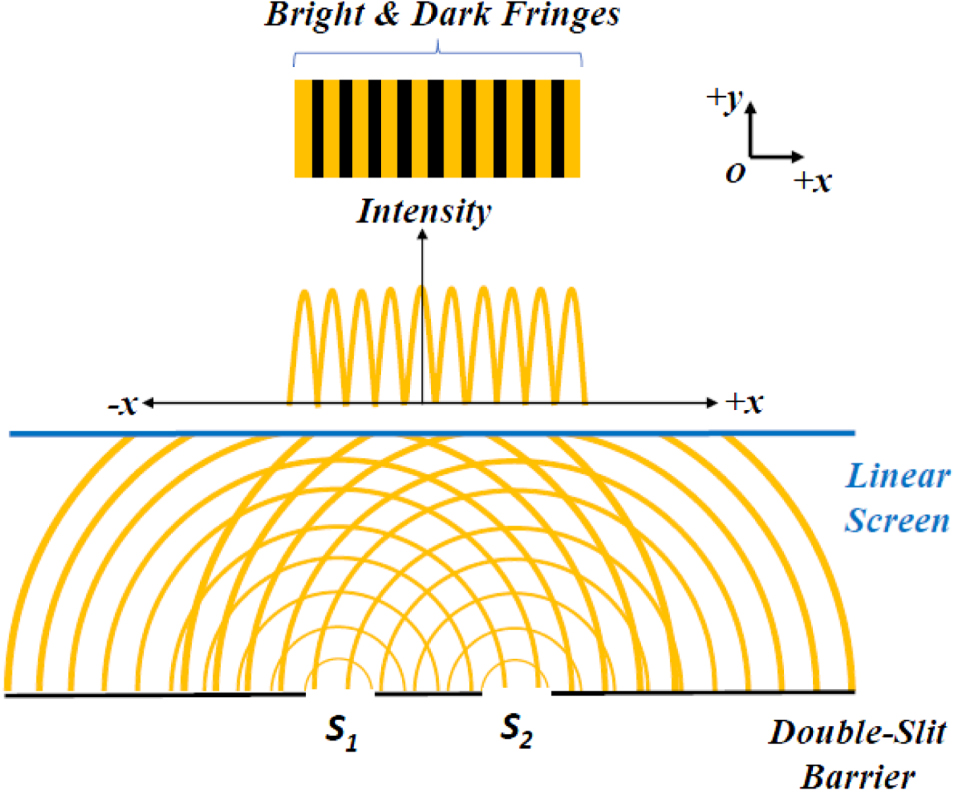
The double slit experiment was historically the first to decisively demonstrate and establish the wave nature of light. It helped bring to rest the then long-standing debate on whether light had a particle or a wave nature [1–4]. In its bare essence, the apparatus consists of a barrier with two very narrow slits S1 and S2, and a screen placed at a suitable distance from the slit barrier. The two slits act as coherent sources emanating circular ripples of light that interfere with each other to produce a pattern of alternating bright and dark bands called fringes on the distant screen (see figure 1). The formation of a bright or dark fringe depends on whether the interference is either constructive or destructive in nature, which in turn depends on the difference in the lengths of the paths taken by light rays from S1 and S2 to reach the particular point P on the screen (see figure 2). The standard formula for path difference (δ) that can be found in many physics textbooks is δ = r1 − r2 = d sin θ, where d is the inter-slit distance, r1 and r2 are the distances of the arbitrary point P on the screen from slits S1 and S2, respectively and θ is the angle as shown in figure 3 [5–8]. In the coordinate reference system chosen, the origin O lies midway between the slit sources and the positive axes directions are as indicated in the figure inset.

Figure 1. Slits S1 and S2 act as coherent sources emanating circular ripples that interfere with each other giving rise to an alternating bright and dark fringe pattern on the distant screen. The distance separating any two successive circular ripples from the same source is the wavelength of light λ.
Download figure:
Standard image High-resolution image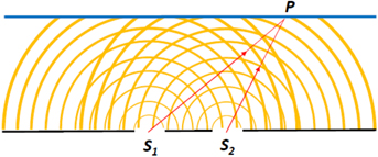
Figure 2. S1P and S2P are light rays emanating from slits S1 and S2 that meet at a point P on the distant screen.
Download figure:
Standard image High-resolution image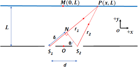
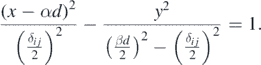
Figure 3. L is the slit-barrier-screen distance, O(0, 0) is the origin, M(0, L) is the center of the screen, P(x, L) is an arbitrary point on the screen where light rays S1P and S2P meet, S1S2 = d is the inter-slit distance,  and
and  are the slit source positions. ∠S1S2N = θ, ∠S2NS1 = 90° and the positions of the points O, M and P are indicated by red dots.
Download figure:
Standard image High-resolution imageThe calculation of δ is based on a pair of assumptions (namely, L ≫ d and d ≫ λ), collectively referred to here as the parallel ray approximation (PRA), that help simplify the geometry of the slit barrier-screen arrangement. The shortcomings of this approach have been discussed previously in regards to its ability to accurately predict the positions of the fringes formed on the distant screen [4]. Some recently published papers however, offer a deeper treatment that make use of the equation of a hyperbola as the locus of points with a given path difference, from which an asymptotic expression is approximated to determine the fringe position [9–12]. While these later approaches circumvent the paradoxical use of PRA, none of them derive the hyperbola equation from first principles. In the new formulation put forward by Thomas (2019), a hyperbola theorem for two slit sources was stated and proved using analytical geometry and differential calculus. It was then suitably employed to determine the exact fringe positions on distant screens of varied shapes, namely, linear, semi-circular and semi-elliptical [4]. This paper carries that prior work further by examining both the qualitative and quantitative aspects of the distribution of interference fringes. Additionally, two equivalent laws of proportionality are predicted that govern the distribution of fringes independent of screen shape. These laws are in principle, amenable to experimental testing.
1.2. The new analysis revisited
In prior work by the author, the following hyperbola theorem for two point sources was stated and proved [4]: the locus of the points of intersections of two uniformly expanding circular wavefronts emanated from two point-sources A(−a, 0) and  separated by a finite distance 2a (where a > 0), propagating outwards with a steady speed u and having a time difference of emanation ΔtAB, is the branch of a hyperbola (see figure 4). Its analytical equation is given by (N.B. the origin lies midway between the point sources),

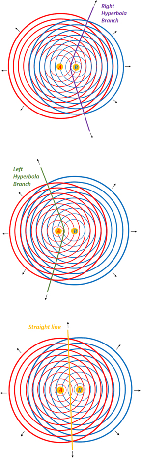
Figure 4. When source A emanates a circular ripple before source B (i.e. tA < tB; ΔtAB = tB − tA > 0), the right branch of a hyperbola is generated (purple) and when source B emanates a circular ripple before source A (i.e. tB < tA; ΔtBA = tA − tB > 0), the left branch of a hyperbola (green) is generated. When sources A and B emanate circular ripples simultaneously (i.e. tA = tB; ΔtAB = tB − tA = 0), a straight line (yellow) is generated. The black arrows indicate the direction of radial expansion and the locus traced.
Download figure:
Standard image High-resolution imageThe above hyperbola theorem was then directly applied to the double slit scenario by treating the two narrow slits S1(−d/2, 0) and S2(d/2, 0) as equivalent to two coherent point sources A(−a, 0) and  . Equation (1a) when rewritten in terms of the path difference δ and the inter-slit distance d takes the following form:

The shape of the screen used to capture the interference fringes was varied (linear, semi-circular and semi-elliptical) and the angular position formulae in each case calculated (see figure 5). An important prediction of the new analysis is that the interference fringes are non-uniformly distributed on each type of screen. That is, they are unequally spaced and of unequal widths. In fact, there occurs narrowing and crowding of fringes near the center of the screen, and widening and dispersal towards the periphery. This is in direct contrast to the PRA-based analysis which predicts uniformity in both the spacing and width of the fringes.
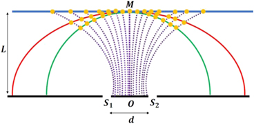
Figure 5. Interference bright fringes (yellow circles) are formed where the family of confocal hyperbolas (purple) intersect the three different shapes of screens [linear (blue), semi-circular (green), semi-elliptical (red)], with the center in common M placed at a distance L from the origin O. Note the crowding of fringes near M and their dispersal towards the periphery.
Download figure:
Standard image High-resolution image2. Formal definitions
This paper undertakes the task of laying the mathematical framework necessary for counting interference fringes formed on screens of different shapes and to draw comparisons in their distributions by means of numerical–graphical simulation using MATLAB software package. Two novel distribution functions called fringe density and fringe dispersion are introduced in order to denote the magnitude of crowding and spreading of fringes on the distant screen, respectively.
2.1. Fringe density
Refers to the number of interference fringes formed on a screen of a given shape per unit length and is denoted by the Greek letter ρ. It may be defined for a particular point on the screen or as an average measure over an interval length.
2.1.1. Point fringe density
Let n and n + Δn be the number of fringes that lie between the center M(0, L) and two peripheral points P1(x, y) and P2(x + Δx, y + Δy) on a screen of a particular shape. Also, let s and s + Δs denote the lengths of the segments MP1 and MP2 on that screen, respectively (see figure 6). Then, we may write the fringe density at a point (x, y) as


Figure 6. n and n + Δn are the number of fringes that occupy segments s and s + Δs of the different screens, respectively. Measurements are made from the common center M along the direction of screen length. Therefore, Δn fringes occupy the segment Δs. (N.B. For the sake of visual clarity, the two peripheral points P1 and P2 are marked only on the linear screen).
Download figure:
Standard image High-resolution image2.1.2. Average fringe density
Let n be the number of fringes that lie between the center M(0, L) and a peripheral point P(x, y) on a screen of a particular shape and s denote the length of segment MP. Then, we may write the average fringe density over an interval length [0, s] as

Since the interference fringes formed on each of the screen shapes shown in figure 7 are symmetrically distributed about the center M(0, L), we may extend the above definition in these cases to the expanded interval [−s, s]:

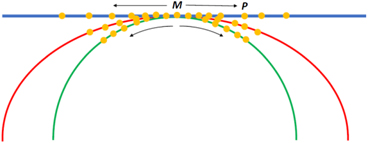
Figure 7. Symmetrical distribution of fringes about the common center M for linear (blue), semi-circular (green) and semi-elliptical (red) screens.
Download figure:
Standard image High-resolution image2.2. Fringe dispersion
Refers to the separation distance between two successive interference fringes formed on a screen of a given shape and is denoted by the Greek letter σ. It may be defined for a particular point on the screen or as an average measure over a fringe interval. Formally written, the fringe dispersion is the reciprocal of fringe density. That is,


3. Fringe distribution analysis--a continuous variable approach
In the subsequent sections, n and s are treated as continuous variables. They can be expressed as functions of the coordinate variables x and y of an arbitrary point on a distant screen of a particular shape, i.e.  and
and  . By the definition of a differential function,

And by the definition of a differential arc segment length,

On substitution of (3a) and (3b) in (2a), we arrive at the (generic) point fringe density formula,
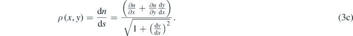
The corresponding dispersion formula is obtained by taking the reciprocal of (3c).
4. Calculation of n(x, y) from the hyperbola theorem
For a two slit-source barrier, the equation of the hyperbola in terms of path difference δ and inter-slit distance d is given by (1b). On rearranging (1b), we get the following biquadratic equation in δ2:

Solving for δ2,

By writing δ as some positive real number multiple n of the wavelength λ (i.e. δ = nλ) in (4b), n may be expressed as

Differentiating n(x, y) partially with respect to x and y,


Where P(x, y) and Q(x, y) are algebraic functions of the coordinate variables x and y:


5. Point fringe density formulae for screens of different shapes
5.1. For a linear screen
Let the analytical equation representing the linear screen with center M(0, D) lying at a distance L = D from the double slit barrier be (see figure 8(A)),

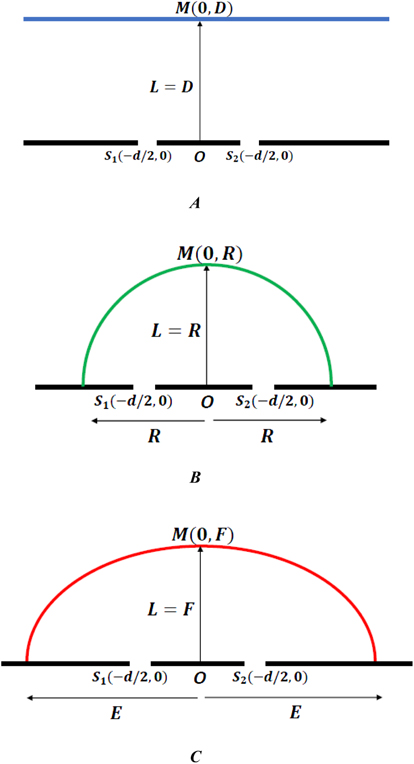
Figure 8. (A) Linear screen placed at a distance L = D from origin O(0, 0). (B) Semi-circular screen placed at a distance L = R (radius) from origin O(0, 0) and R > d/2. (C) Semi-elliptical screen placed at a distance L = F (semi-minor axis) from origin O(0, 0) and E > d/2 (semi-major axis).
Download figure:
Standard image High-resolution imageDifferentiating (5.1a) with respect to x (D is a constant),

Substituting (5.1a), (5.1b), (4d), (4e) in (3c),

5.2. For a semi-circular screen
Let the analytical equation representing the semi-circular screen with center M(0, R) lying at a distance L = R from the double slit barrier be (see figure 8(B)),

The semi-circular screen is part of a whole circle with center O(0, 0) lying midway between the two slits  and with radius R > d/2. Differentiating (5.2a) with respect to x (R is a constant),

Substituting (5.2a), (5.2b), (4d), (4e) in (3c),

5.3. For a semi-elliptical screen
Let the analytical equation representing the semi-elliptical screen with center M(0, F) lying at a distance L = F from the double slit barrier be (see figure 8(C)),

The semi-elliptical screen is part of a whole ellipse with center O(0, 0) lying midway between the two slits  , having axes of lengths E&F along the x & y-axes, respectively and with E > d/2. Differentiating (5.3a) with respect to x (E&F are constants),

Substituting (5.3a), (5.3b), (4d), (4e) in (3c),

5.4. Central fringe density
The magnitude of the point fringe density at the screen center M(0, L) can be found by substituting  in (5.1c), (5.2c) and (5.3c), where L is equivalent to D, R or F for the respective screen shape (refer subsection 12.1 of the mathematical appendix for the evaluation of
  ). The central fringe density takes the same form in all three cases,

6. Average fringe density formula over a fringe interval or length interval on a linear screen
Consider a linear screen with n fringes lying between the center M(0, D) and an arbitrary point P(x, D) in the periphery. The average fringe density formula may be written based on definition (2c) as

On substitution of the analytical equation of the linear screen (5.1a) into the hyperbola theorem (1b) and rearrangement of terms, we get

Expressing the path difference δ in (6.2) as some positive real number multiple n of wavelength λ (i.e. δ = nλ),

Dividing (6.3) by 'n2',


In (6.5), ρav is defined over the fringe interval [−n, n], where n is bounded by the upper and lower limits  (i.e.
(i.e.  ). But ρav can also be defined over the length interval [−x, x] where x is unbounded, by replacing nλ with δ in (6.5) and then inserting the expression for δ2 given in (4b),
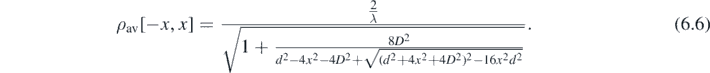
Upon substitution of n = 0 in (6.5) or x = 0 in (6.6), we get a result that is identical in form to (5.4). This implies that at the center of the linear screen, the average fringe density is exactly equal to the point fringe density. Without foraying into the extensive calculations, it can be shown that the formulae for average fringe density over an interval length of a semi-circular and semi-elliptical screen also shares the same corresponding (inverse) relationship with the wavelength λ.
7. Laws of fringe distribution
A careful inspection of the set of equations for point fringe density in the case of a linear screen, a semi-circular screen, a semi-elliptical screen {(5.1c), (5.2c), (5.3c)} and the average fringe density for a linear screen {(6.6)} reveals a quantitative relationship that is screen shape invariant and point-interval invariant, namely,  . Since the wavelength λ is related to the frequency ν and the speed of light c by the expression c = νλ = constant, it logically follows that ρ ∝ ν. Also, based on the definition of fringe dispersion (subsection 2.2),
  . We may thus, write the following proportions for any two frequencies ν1 & ν2 (or wavelengths λ1 & λ2) in the electromagnetic spectrum, with respective fringe densities ρ1 & ρ2 and fringe dispersions σ1 & σ2:

These two equivalent laws of proportionality (i.e. ρ ∝ ν and σ ∝ λ) are in principle, amenable to experimental testing.
8. Miscellaneous remarks
8.1. On central fringe density
8.1.1. Factors of dependence
An inspection of (5.4) reveals that ρ(0, L) depends on only two factors: firstly, the wavelength (λ): this is a characteristic of the source. By increasing the wavelength (or equivalently, decreasing the frequency) of light emitted by the source, the central fringe density decreases. Secondly, the ratio of the slit barrier-screen distance to the inter-slit distance ( ratio): this is a characteristic of the geometry of the slit barrier-screen arrangement. By increasing this ratio, the central fringe density decreases.
8.1.2. Far-field and near-field approximations
Here, we define the far-field and near-field limits as L ≫ d and L ≪ d, respectively. Using the binomial theorem for rational exponents and neglecting all higher power terms of d/L or L/d that are greater than or equal to 2, the following approximations for central fringe density are arrived at.
- (a)In the far-field limit (L ≫ d)

- (b)In the near-field limit (L ≪ d)
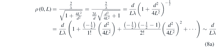
Based on the definition of fringe dispersion (subsection 2.2), we can infer the following from (8a) and (8b): firstly,  in the far-field limit. This result agrees well with the PRA-based analysis of the double slit experiment which predicts uniform fringe widths and inter-fringe spacings for all orders of fringes when L → ∞ (both bearing a magnitude of
  ). Secondly,
  in the near field limit. This result agrees well with the prediction that standing waves are produced along the axis connecting the two sources when L → 0 (the maxima are separated by
 ).
).
8.2. for a semi-circular and semi-elliptical screen

Upon substitution of E = F = R and x2 + y2 = R2, (5.3c) is reduced to (5.2c). This shows that the point fringe density formula derived for the semi-circular screen is simply a special case for that of the semi-elliptical screen.
8.3. On the defining formulae of and


An inspection of the set of equations {(5.1c),(5.2c),(5.3c)} reveals that  can be either a positive or a negative quantity depending upon the sign that the x-coordinate takes, while the y-coordinate always remains positive. This would imply that the sign of ρ indicates the position of point
  relative to the screen center
  . That is, if ρ > 0 then P lies to the right of M and if ρ < 0 then P lies to the left of M. An absolute value function may therefore, be appropriately introduced on the right-hand side of the defining formulae {(2a), (2d)} for fringe density and dispersion in order to emphasize magnitude instead of relative position. That is,
 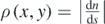 and
and 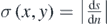 .
.
9. Numerical-graphical simulation using MATLAB
The following numerical values  are adopted (in SI units) for the purpose of graphical simulation of the point fringe density formulae for different screen shapes {(5.1c), (5.2c),(5.3c)}, and the average fringe density formula for a linear screen {(6.6)}. These values fall within the conventional range that the double slit experiment is carried out in the laboratory. In figure 9(A), the point fringe density is observed to decrease from the center to the periphery fastest for the linear screen (blue), intermediate for the semi-elliptical screen (red) and slowest for the semi-circular screen (green), as indicated by the slopes of the bell-shaped curves. The central fringe density for all three screen shapes have the same magnitude (8000 fringes/m). In figure 9(B), a similar trend is observed for the average fringe density on a linear screen. It is to be noted that the central fringe density for both the average and the point measures are exactly equal. The fringe dispersion behavior can be inferred by considering a direct inversion of these graphs. Accordingly, the rate at which the fringes spread apart increases from center to periphery fastest for the linear screen, intermediate for the semi-elliptical screen and slowest for the semi-circular screen. The simulation results that are obtained here match the schematic construction presented in figure 5.

Figure 9. (A)  fringes/m for λ = 500 nm. (B)
  fringes/m for λ = 500 nm.
Download figure:
Standard image High-resolution image10. Fringe distribution analysis--a discrete variable approach
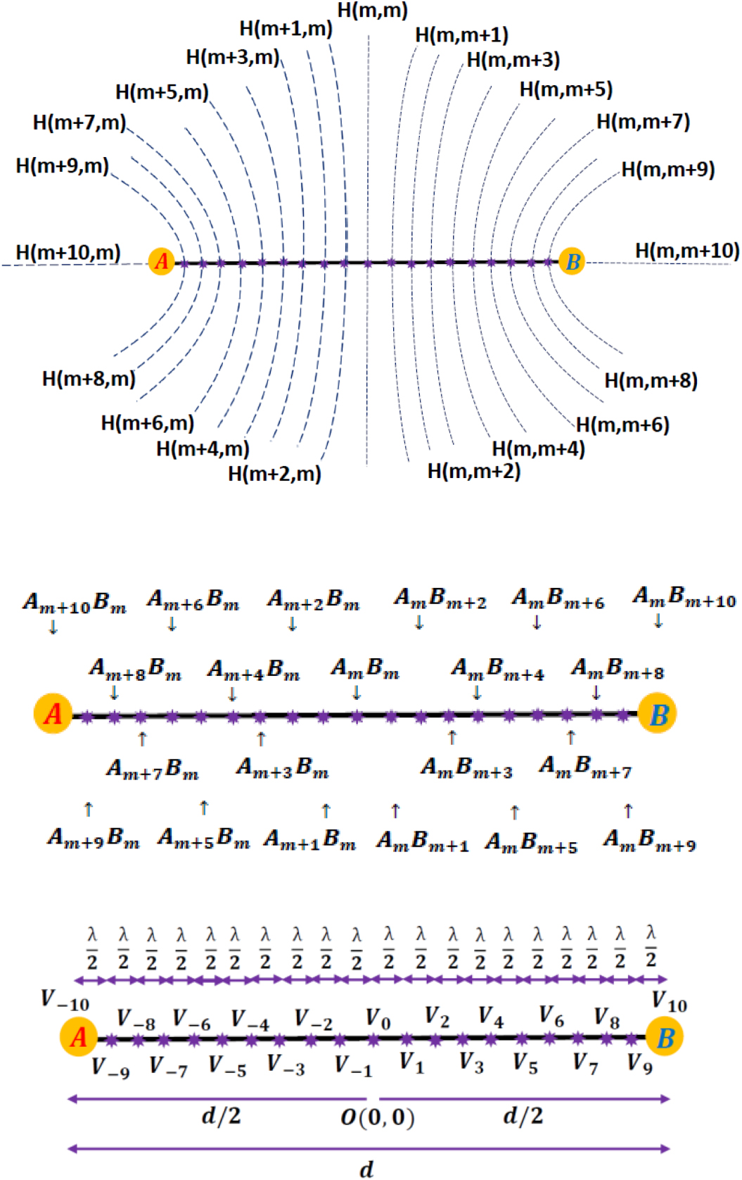
10.1. Numbering successive wavefronts: wavefront order
Consider two coherent point-sources A(−d/2, 0) and B(d/2, 0) that emanate concentric circular wavefronts radially outwards with a uniform speed u (N.B. point sources are an idealization of narrow slits). Pairs of wavefronts that are emanated simultaneously from their respective source centers may be sequentially numbered in the order of their emanation. For instance, the first pair of wavefronts emanated from A and B are labelled '1', the second pair are labelled '2' and so on. The separation distance between any two successive wavefronts from either source is equal to the wavelength λ. The wavefront orders, denoted by the letters p and q for A and B respectively, may be defined using set theoretic notation as follows:  and
and  (see figure 10).
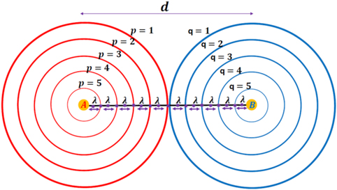
Figure 10. p and q are the wavefront orders for sources A and B, respectively; d is the inter-source distance and λ is the inter-wavefront distance (i.e. wavelength). The purple stars marked along the length of the line segment AB denote the points of pairwise meeting of red and blue wavefronts.
Download figure:
Standard image High-resolution image10.2. Numbering successive hyperbola vertices: vertex order
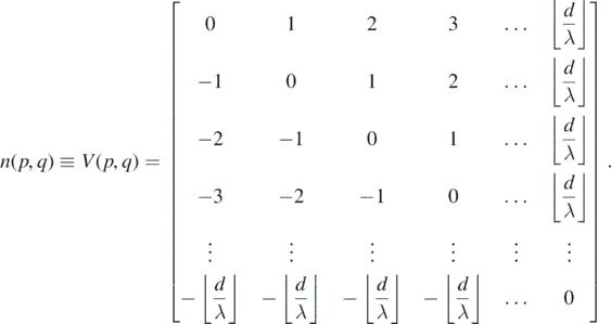
When the pth circular wavefront from A meets and intersects the qth circular wavefront from B, a hyperbola branch is traced out and it may be symbolically specified as H(p, q) ≡ ApBq (see figure 11). The hyperbola vertex is situated where the two wavefronts meet at a point along the length of the intervening line segment AB. The vertex may be numbered based on the wavefront orders p and q. The vertex order, denoted by the letter V, is defined by the formula V = −(p − q). Thus, for  and
and 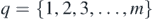 ,
,  . Here,
  is the floor function (also known as the greatest integer function). The various semi-hyperbolas
  may be written out as a matrix array with p as the row number and q as the column number to which a specific branch belongs (see subsection 10.9).

Figure 11. The various orders of wavefronts  , emanated from sources A and B meet at specific points on the line segment AB (marked by purple stars). Each meeting point represents a hyperbola vertex and adjacent vertices are spaced λ/2 distance apart. In the depicted example, ten half-wavelengths are accommodated in one half of the inter-source distance. Hence, ⌊d/λ⌋ = 10.
Download figure:
Standard image High-resolution image10.3. Numbering successive fringes: fringe order
Bright fringes are formed on a distant screen where constructive interference occurs between waves from sources A and B. But based on our current geometrical framework, a fringe may also be said to be located where the hyperbola branch H(p, q) ≡ ApBq intersects the screen (see figure 12). And since each hyperbola branch has an associated vertex, it implies that every fringe formed on the screen is simply a projection of a corresponding vertex that lies on the line segment AB. This further implies that there are as many bright fringes as there are hyperbola vertices. Hence, an exact point-to-point correspondence exists between the ordering of fringes and the ordering of vertices (topographic representation). We are therefore, justified in writing the fringe order n as equivalent to the vertex order V, i.e. n ≡ V = −(p − q). For the single bright fringe that is formed at the screen-center (central maxima), n = 0 and for the two bright fringes formed at the screen extremities (peripheral maximas),  .
.
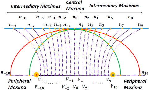
Figure 12. The bright fringes are projections of the hyperbola vertices onto the distant screens (linear, semi-elliptical, semi-circular). In the depicted example, the single central maxima and the two peripheral maximas are of fringe orders n = 0 and n = ±10, respectively while the intermediary maximas are of fringe orders{±1, ±2, ..., ±9}.
Download figure:
Standard image High-resolution image10.4. Distance relations
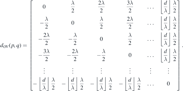
A complete quantitative treatment pertaining to the counting of fringes can be found in the supplementary material (https://stacks.iop.org/EJP/41/055305/mmedia) of this paper. Only a summary of the principal theoretical results is presented in the subsequent sections. For a semi-hyperbola H(p, q) ≡ ApBq with vertex order V = −(p − q), let rA and rB be the instantaneous radii of the pth order and qth order circular wavefronts the moment they just meet at a point V along the line segment AB (see figure 13). Also, let dOV be the distance of the hyperbola vertex V from the origin O. It can be shown that the following distance relations hold true at the meeting point V:


Figure 13. Circular wavefronts from sources A(−d/2, 0) and B(d/2, 0) with orders p = m1 and q = m2 meet at point V when their instantaneous radii are rA and rB, respectively. (N.B. m1 < m2 and rA > rB)
Download figure:
Standard image High-resolution image10.5. Maximum fringe order and maximum vertex order
The maximum fringe order nmax or equivalently, the maximum vertex order Vmax can be shown to be

10.6. Total fringe count and total vertex count
The total number of fringes (Ω) formed on the distant screen or equivalently, the total number of hyperbola vertices that occur on the line segment AB can be shown to be

10.7. Special cases
From (10.3), it is clear that the total fringe count (Ω) depends on the relative magnitudes of the inter-source distance and the wavelength of light (i.e. the  ratio). There are therefore, three possible cases to consider in turn: λ > d; λ = d; λ < d (see table 1).
Table 1. The geometrical relationship of Ω and d/λ ratio.
| Case | Ω | Geometrical interpretation | n |
|---|---|---|---|
| (i) λ > d | 1 | 1 central maxima | {0} |
| (ii) λ = d | 3 | 1 central maxima | {0, ±1} |
| + 2 peripheral maximas | |||
| (iii) λ < d | |||
(a)  |  | 1 central maxima + 2 peripheral maximas +  intermediary maximas intermediary maximas | 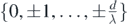 |
(b)  |  | 1 central maxima + 2 peripheral maximas +  intermediary maximas intermediary maximas |  |
10.8. Maximum wavefront order
The maximum wavefront order pmax of a circular wavefront emanated from source A that can meet and intersect with a circular wavefront from source B of wavefront order q = m along the line segment AB, is  , where
  . Similarly, the maximum wavefront order qmax of a circular wavefront emanated from source B that can meet and intersect with a circular wavefront from source A of wavefront order p = m along the line segment AB, is
  . Formally stated, for
 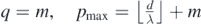 , and for
 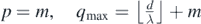 .
.
10.9. Matrix array representation
All the theoretically arrived at results in section 10, may be conveniently represented in compact form using square matrix arrays. In these m × m matrices, the wavefront orders p and q are employed to designate the row and column numbers, respectively.
10.9.1. Hyperbola matrix
The members of the family of confocal hyperbolas that are generated from the intersections of m circular wavefronts emanating from source A with m circular wavefronts emanating from source B, may be collectively written as
10.9.2. Fringe order or vertex order matrix
The various orders of bright fringes and hyperbola vertices may be collectively written as
10.9.3. Vertex position matrix
The distances of the various hyperbola vertices from the origin O(0, 0) may be collectively written as
11. Summary and concluding remarks
By establishing in this paper, a rigorous framework for the counting of fringes formed on screens of varied shapes, two significant departures from the predictions of the PRA-based analysis of the double slit experiment are demonstrated. They concern namely, the fringe widths and the inter-fringe spacings. While the conventional textbook approach predicts uniformity of fringe widths and inter-fringe spacings for all orders of fringes, the new analysis predicts non-uniformity in both these parameters. This is evident from the numerical–graphical simulation of ρ(x, y) which shows firstly, that the fringes are more crowded together near the center of the screen and spread apart towards the periphery (see figure 9(A)). And secondly, the rate of dispersion of the fringes from center to periphery is highest for the linear screen, intermediate for the semi-elliptical screen and lowest for the semi-circular screen, when all three types of screens are placed at the same distance from the double slit barrier. Similar trends can be observed in the average measures for a linear screen (see figure 9(B)).
The two distinct approaches employed for analysing the fringe distributions may be contrasted in the context of the results obtained. In the continuous variable approach (sections 3–9), a quantitative assessment of the degree of non-uniformity of fringe distributions (as encapsulated by the functions ρ and σ) for different screen shapes is elucidated. Whereas in the discrete variable approach (section 10), an absolute count of the total number of fringes (Ω) is calculated. In other words, the latter approach provides a global measure for the population size of the fringes formed for a given slit-source separation (d) and wavelength of light (λ), while the former approach renders a local estimate of the point to point variations in the distribution of that population along the length of each screen type.
On an additional note regarding the total fringe count, both the new and the conventional analysis concur that a finite upper bound exists which is determined by the ratio of the inter-slit distance to the wavelength of light. However, the geometrical approach employed here to reach this parallel conclusion involves radially expanding circular wavefronts instead of an error prone approximation formula for path difference, thereby affording a more precise and paradox free scheme. Furthermore, the principal theoretical results obtained for 2-slit interference can be readily extended to the case of N-slit interference (see subsection 12.2 of the mathematical appendix). The new analysis also has the distinctive pedagogic advantage of being more visually intuitive. This author therefore, suggests that its core concepts and ideas be incorporated into the undergraduate physics curriculum, to be taught alongside the conventional approach.
A final assertion forwarded herein are the two laws of fringe distribution that are screen-shape invariant and point-interval invariant. A formal statement that combines both laws is as follows: 'In the classical double slit experiment, regardless of the shape of the distant screen used to capture the interference pattern, or whether a point or interval measure is sought after, the density of fringes formed on the screen is directly proportional to the frequency of light and the dispersion of fringes is directly proportional to the wavelength of light'. These optical relations are a means to experimentally test the validity of the mathematical theory presented in this paper, and if proven true, may have a significant bearing on the science of interferometry. All of the key predictions summed up here will be best evident when the inter-slit distance is made comparable to the wavelength of light used. Though this may be difficult to achieve in the laboratory with visible light (400 nm–700 nm) owing to the very small wavelengths involved, it may be more readily demonstrated using microwaves (1 mm–1 m). An experiment that is suitably designed towards this end is therefore, highly recommended to opticalresearchers.
12. Mathematical appendix
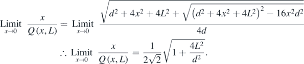
12.1. Evaluation of

The expression  takes the indeterminate form
  as x → 0 and therefore, requires a few simple manipulations before the direct substitution of x = 0 to ascertain the limit. Since the denominator contains an algebraic surd, the first step is to rationalize the denominator.
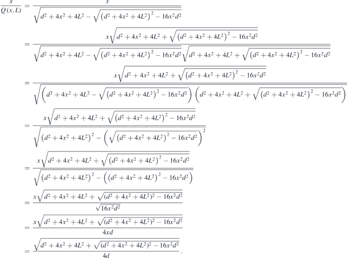
Applying  on both sides,
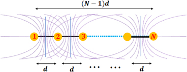
12.2. Fringe counting for N-slit interference
Consider the scenario wherein there are N-coherent point sources (N ⩾ 2) spaced equally apart along a straight line and are serially numbered 1, 2, 3, ..., N (see figure 14). Let d be the distance between any two adjacent sources and λ the wavelength of light emanated from each of them. The interference of circular wavefronts from the N sources results in the generation of a family of families (i.e. a community) of confocal hyperbolas. Any given pair of sources (i, j), where i, j ∈ {1, 2, 3, ..., N} and i ≠ j, act as common foci for all the members of a particular family. The analysis that was previously carried out for 2-sources in section 10 may be extended to the N-sources case. The analytical equation of the community of confocal hyperbolas was first presented in [4] and is repeated again below:
Figure 14. A community (i.e. a family of families) of confocal hyperbolas for adjacent source pairs. For the sake of visual clarity, the families between non-adjacent source pairs are not depicted.
Download figure:
Standard image High-resolution image
Here, α and β are the coefficients of translation defined as  and β = j − i subject to the constraint j > i ; δij denotes the path difference between the rays arising from sources i and j. The above generalized hyperbola equation reduces back to the two-source scenario (equation (1b)) upon substituion of i = 1 and j = 2. (N.B. The origin of the coordinate reference frame is chosen to lie midway between the sources 1 and 2).
12.2.1. Total fringe count and total vertex count
The total number of bright fringes formed on a distant screen (or equivalently, the total number of hyperbola vertices that occur on the line joining the two extreme most sources 1 & N) has an upper bound given by

Here, m is the index of summation and C is the combinatorial function. The geometrical interpretation of the above inequality is as follows: the first summation term represents the total number of peripheral maximas and the second combinatorial term represents the total number of central maximas. The reason for the employment of an inequality symbol is to account for the possible spatial overlap of some of the maximas for different source pairs.
12.2.2. Max. fringe order & max. vertex order
For any pair of sources (i, j), the maximum fringe order (or equivalently, maximum vertex order) is given by
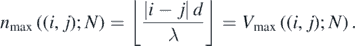
Here,  is the absolute value function.
12.2.3. Maximum wavefront order
For any pair of sources (i, j), the maximum wavefront order pmax(i) of a circular wavefront emanated from source i that can meet and intersect with a circular wavefront from source j of wavefront order q(j) = m along the line segment AB, is  , where
  . Similarly, the maximum wavefront order qmax(j) of a circular wavefront emanated from source j that can meet and intersect with a circular wavefront from source i of wavefront order p(i) = m along the line segment AB, is
  . Formally stated, for
  , and for
  .
.
Acknowledgments
Gloria in excelsis Deo.