

Abstract
The geodynamo usually appears as a somewhat intimidating subject. Its understanding seems to require knowledge of the intricate theory of magnetohydrodynamics. The solution of the corresponding equations can only be achieved numerically. It seems to be a subject for the specialist. We show that one can understand the basics of the functioning of the geodynamo solely by using the well-known laws of electrodynamics. The topic is not only important for geophysicists. The same physics is the cause for the magnetic fields of Sun-like stars, of the very strong fields of neutron stars, and also of the cosmic magnetic fields.
Export citation and abstract BibTeX RIS

Original content from this work may be used under the terms of the Creative Commons Attribution 4.0 licence. Any further distribution of this work must maintain attribution to the author(s) and the title of the work, journal citation and DOI.
1. Introduction
In physics lectures, the geodynamo is usually only briefly mentioned, although it is a very interesting topic. It gives rise to the well-known magnetic field of the Earth. However, not only the Earth and other planets have magnetic fields, but also all Sun-like stars, white dwarfs, and neutron stars. The magnetic field of some neutron stars, the magnetars, is so strong that a liter of it has a mass of many metric tons. On the other side, there are the cosmic magnetic fields which have very low field strengths but are of gigantic extensions. All of these fields are generated in essentially the same way as that of the Earth's. We believe that the 'mechanism' by which these fields are created should not only be a subject for the specialist, i.e. the geophysicist or the astrophysicist. It should be treated at school, and at the university in the normal physics lecture.
The origin of the Earth's magnetic field, or in other words, the functioning of the geodynamo, seems to be a difficult subject. To fully understand it, one needs the theory of magnetohydrodynamics, which is justifiably feared, since it combines the difficulties of electrodynamics with those of hydrodynamics. And even using these theories, it seems that the final answer to the question of how the geodynamo works can only be obtained by means of extensive numerical calculations.
What the students typically learn can be summed up in a few sentences.
The magnetic field of the Earth does not originate from a permanent magnet, because the temperature inside the Earth is too high. It is caused by electric currents which are generated in the same way as with a self-excited dynamo: by the movement of an electrical conductor in a magnetic field. This 'geodynamo' is driven by the thermal convection of the liquid iron inside the Earth.
However, the question of how the currents come about, i.e. how the geodynamo works, is more difficult to answer. We want to ask this question, but without the high claim to be able to explain the actual field distribution. We only ask: how can such an effect occur in a homogeneous electrical conductor? So we are only looking for a qualitative explanation.
A detailed analysis can be found in Moffatt's book Magnetic Field Generation in Electrically Conducting Fluids [1]. There, a model is discussed which fulfills the above-mentioned requirement: the homopolar disk dynamo. A disadvantage of this model is that the path of the electric current is predetermined by electrical conductors, which is not the case in the homogeneous medium in the Earth's core.
An interesting question that we will not address is why the magnetic field changes direction from time to time. This question is discussed in an easy-to-understand article by Glatzmaier and Olson in Scientific American [2]. There are also impressive magnetic field line pictures created by simulation.
An approach to treating the topic with the means of school physics was presented by Watt and Roth [3]. Of course this approach must leave many questions unanswered. Also in their model, the path of the electrical current is determined by metallic conductors. Another problem that has not been addressed is the fact that a pure translational movement of the liquid iron cannot, in principle, cause a dynamo effect.
An obvious way to become more familiar with the field of the Earth is to measure it, including its vertical component. This is done by Amiri and Jeffery [4].
Our approach lies somewhere between the secondary school teaching on the one hand and the lectures for specialists on the other [1, 5], i.e. an approach that fits into the physics lecture at the university. It takes about 1 h of lecturing.
In particular we address the following questions.
- With the self-excited dynamo, the path of the electric current through the conductors is well-defined, as is the movement of the conductors. How is it possible that a dynamo effect takes place when the electric current is allowed to flow 'as it likes' and the conductors can move 'as they like'?
- We know that the technical dynamo has to be started. Who had started the geodynamo?
- Why does the dynamo effect exist in the Earth (and other celestial bodies), but not in systems of our everyday environment?
In section 2 we will describe the phenomenon: the structure of the Earth and the structure of the magnetic field. Section 3 explains how the geodynamo is working. However, it will not yet be clear under which circumstances the geodynamo effect actually occurs. This question is clarified in section 4. Finally, it is still to be discussed how the dynamo is started. This will be done in section 5. In section 6 our results are summarized.
2. The structure of the Earth and of its magnetic field
2.1. The Earth
Figure 1 shows a cross-section of the Earth. The core, which has a radius of 3480 km, consists mainly of iron and is electrically conductive. (The conductivity is about 1/10 of that of iron under normal conditions.) The mantle consists of rock whose electrical conductivity is about 5 orders of magnitude smaller. We can consider it an insulator. The inner core with a radius of 1210 km is solid, the outer core is liquid. The viscosity of the iron in the outer core is not very different from that of liquid iron on the Earth's surface. The viscosity of the mantle, on the other hand, is so high that we can consider it solid. The temperature in the core and mantle decreases from the inside to the outside. In the center of the Earth, it is about 6000 K, at the surface of the core it is slightly more than 4000 K. Since a heat transport takes place from inside to outside, the Earth cools down slowly. This cooling process, however, has a duration comparable to the age of the Universe. We can, therefore, assume a temperature gradient from the inside to the outside that is constant in time on timescales relevant to the dynamo process.
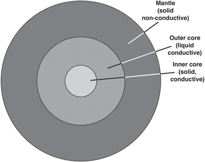
Figure 1. The structure of the Earth. The outer core meets the conditions for the dynamo effect to occur: it is liquid and electrically conductive.
Download figure:
Standard image High-resolution imageIn the region we are interested in, namely the outer core the heat is transported by convection: the liquid metal moves at a speed of a few km a−1. (Compared to other 'geological' velocities, such as those of the continental plates, this velocity is quite high.) However, this convection current is not simply up and down. Due to the rotation of the Earth, any translational motion is overlaid by a rotational motion, a phenomenon that we know from the air currents in the atmosphere. Altogether we have a screw-shaped motion.
2.2. The field
Where the field can be easily observed, i.e. outside of the Earth, it is approximately a dipole field, similar to the field of a bar magnet or a cylindrical coil. But inside of the Earth, the spatial distribution of the field strength is far from being that of a dipole field. Figure 2 shows calculated field lines [2, 6]. It has an irregular and intertwined structure with variations on a length scale of about 100 km. For more recent calculations of the magnetic field see for example [7].
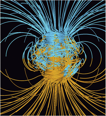
Figure 2. Calculated magnetic field. In the Earth's core it is irregular and intertwined. Reproduced with permission from [5].
Download figure:
Standard image High-resolution image2.3. The temporal development
3. The mechanism of generating the magnetic field
3.1. The technical self-excited generator
The geodynamo basically works like a self-excited technical, i.e. artificial generator. Let us briefly recall how such a generator works. The stator is an electromagnet that creates the magnetic excitation field. A current is induced in the rotor coil, which rotates in the stator field. This same current is passed through the stator coil.
The self-excited dynamo has some characteristics that we also find in the geodynamo, and which we would like to highlight here.
- In order for the self-excited dynamo to start, the stator must first be supplied from another source, because as long as no current flows in the stator coils, no current is induced in the rotor coils.
- If the dynamo runs too slowly, it can 'extinguish'.
- If the rotor runs sufficiently fast, an arbitrarily small magnetic field is sufficient to start the dynamo effect. The faster the dynamo runs, the more unstable becomes the currentless state.
3.2. How the geodynamo does not work
For an artificial dynamo, the path of the electrical current is well-defined, as is the movement of the electrical conductors. The Earth achieves the same result, although the conductors seem to move without any plan, and although the electric current has no predetermined paths. In order to understand how it performs this miracle, let us first discuss a situation in which there is no dynamo effect, and understand the reason for it.
In the following we will look at the fields at one position. We are not asking how these fields are related to those in the neighborhood. So we will not be able to make any statements about the distribution of the field in space. In addition, we are only looking at one point in time. This means that the processes that we present in the following as a causal chain take place simultaneously at the same place. One can also see it that way: we break down a complex process into additive components or contributions. Or more precisely: we break down the relevant vector quantities velocity, magnetic field strength and electric current density into components whose combined action is easier to understand than the process as a whole.
We call the corresponding field strengths B0, B1, and so on. Accordingly, we designate electric currents with j0, j1, ... (the symbol of the current density) and movements with v (the symbol of velocity).
To get a dynamo effect, we have to assume that there is a magnetic field at the beginning. Let us call it B0. We will discuss in section 5 where this initial field may come from. For the moment it is just 'fallen from the sky'. We now hope to get a new magnetic field out of it by a suitable movement of an electrically conductive liquid, so that the induction process continues by itself even though we subsequently switch off the source of B0.
We begin by moving our liquid within the initial field perpendicularly to the direction of the field vector B0, figure 3. (Black arrows represent movements, the red tubular shapes represent the magnetic flux and blue arrows the electric current density vector.)

Figure 3. Movement of an electrically conducting liquid within a magnetic field. The white arrows represent the velocity, the red tubular shapes the magnetic flux and the blue arrows the electric current density vector. A translational movement (a) in the magnetic field B0 results in an electric current j1 (b). The current j1 causes the magnetic field B1 (c). The movement of the liquid in B1 gives rise to the new currents ja and jb. As a result, the total current is shifted upwards. The liquid flow attempts to carry the electric current and the magnetic field with it.
Download figure:
Standard image High-resolution imageThe resulting Lorentz force on the charge carriers causes an electric current perpendicular to B0 and to the velocity according to the right-hand rule. According to Ampère's law this current causes a magnetic field B1. What is the effect of the movement of the liquid in B1? Above j1 the Lorentz force creates a current ja, which flows in the same direction as j1, and below there is a current jb, which flows in the opposite direction. The result of all three currents j1, ja and jb together is an upwards shift of the total current. In other words: the liquid tries to drag the current j1 with it. The greater the electrical conductivity, the better it succeeds in doing so. In the ideal case of a perfect conductor, this effect would be complete: the electric current and the magnetic field would be 'frozen' in the liquid.
But what happens when we now switch off B0? The induced current is displaced a little by the liquid and, at the same time, it decays. There is no dynamo effect. The reason: the movement was too simple.
3.3. How the geodynamo works
In fact, the dynamo effect cannot arise if the velocity field is curl-free or in other words, if there is no shear in the field. We therefore add a second, independent movement to the translational movement: a rotation around the direction of the translational velocity. The result is a helical motion. In the following, we explain how such a movement produces a magnetic field that has the same direction as the initial magnetic field.
Figure 4 shows the process, broken down into 4 separate steps. In each of them we consider only part of the problem: first only the translational component of the movement, then only the rotation, then again only the translation and finally once more the rotation. We also decompose the magnetic field and the electric current density vectors into components and consider only one of them at a time. This is permitted because the different components of the vector quantities magnetic field strength and electrical current density add up linearly and therefore do not influence each other. Of course, we only get a small part of the total solution of the problem. The directions of the arrows in the figure that represent the B and j vectors follow from the well-known right-hand rules.

Figure 4. Translation and rotation cause an initially existing field B0 to be converted into a new field B4, which has the same direction as B0. Although the partial processes all occur simultaneously, they are shown here as a causal chain. This makes the complex overall behavior transparent.
Download figure:
Standard image High-resolution image
Figure 4(a) shows the initial magnetic field B0 and the translational motion of the liquid. This movement within the magnetic field results in an electric current j1, figure 4(b). For the sake of clarity, B0 and the translational motion vtrans are no longer shown in the next figure 4(c). In the following, we are only interested in the effects of the current j1. This current generates a magnetic field, figure 4(c). Figure 4(d) does no longer show j1. Instead, we consider the effects of the rotational motion of the liquid within the field B1. Figure 4(e) sketches the resulting electric current j2. In figure 4(f), B1 and vrot are no longer shown, but instead the magnetic field B2 caused by j2 is represented. In figure 4(g) j2 is omitted and the translational movement is considered again. It leads to a new current j3, figure 4(h). In figure 4(i) B2 and vtrans are no longer shown but instead, the magnetic field B3 generated by j3. Next, the influence of the rotational movement is again taken into account, figures 4(j) and (k): a current j4 is generated. The last picture shows how the magnetic field B4 is generated by j4. The sequence of the cause-effect steps is summarized in table 1.
Table 1. Four steps to obtain a field parallel to the starting field.
| Movement vtrans + field B0 | → | Current j1 |
| Current j1 | → | Field B1 |
| Field B1 + movement vrot | → | Current j2 |
| Current j2 | → | Field B2 |
| Movement vtrans + field B2 | → | Current j3 |
| Current j3 | → | Field B3 |
| Field B3 + movement vrot | → | Current j4 |
| Current j4 | → | Field B4 |
We now have the desired result: B4 has the same direction as B0. So we no longer depend on the original field B0. Our 'dynamo' continues to run, provided, of course, that the liquid moves fast enough.
The representation in figure 4 may have created a false impression. It looks as if we had 'constructed' a stationary dynamo. The figure seems to show how a spiral movement reproduces the initial field B0. It is true that our model shows that such a field is generated. However, that does not mean that the field configuration is stationary. The reason is that we have ignored several other processes. In figure 4(d), for example, we only considered the rotation, but not the translation. The translational movement also generates currents by means of B1, and these, in turn, have their field, etc in figure 4(g), we only considered the effect of the translation, but not that of the rotation. Again, we have disregarded other current components, etc.
Furthermore, we have not taken into account another effect that makes the field more complicated: we have assumed the flow to be given. We imposed it on the liquid. This is not true either. The magnetic fields have an effect on the liquid. The thermodynamic driving engine, i.e. convection, supplies the energy dissipated by the electric currents. It is thus subjected to a braking effect, like an ordinary technical dynamo to which a load is connected. This effect changes the flow of the liquid.
The actual process is therefore, more complex than figure 4 suggests. More intricate structures are created and it cannot be expected that there is a stationary state. What we have looked at is only a small part of the overall picture. However, this contribution is important for an understanding of the geodynamo because we now see that the initial field B0 is no longer needed.
4. Time and length scales
If an electrically conductive liquid is moved sufficiently irregularly electric currents and magnetic fields are generated. A simple experiment that shows this effect, one might think, looks like this: one fills a bucket with saltwater and stirs it, somewhat irregularly. From what has been said so far, we might expect electric currents to start flowing and magnetic fields to be created. But our common sense may also tell us that this will not happen. And, in fact, it is not happening.
The reason why the experiment does not succeed is that the values of some of the parameters on which the effect depends are not large enough. In the following, we will ask what these parameters are
4.1. The lifetime of a current within the core of the Earth
We leave aside the problem of the Earth's magnetic field for a moment and look at an RL circuit: the terminals of a coil (inductance L) are connected to the terminals of a resistor (resistance R). We ask for the behavior of this arrangement when it is enlarged geometrically: when all linear dimensions are multiplied by one and the same factor k. We ask in particular how the decay time will scale. The original decay time being

we ask for the decay time

after the circuit has been enlarged by a factor k. For this purpose, we need to calculate how the resistance and the inductance are scaling.
The resistance R of a geometrically simple resistor can be calculated as

where ρ is the electrical resistivity, l the length and A the cross-sectional area.
Increasing the size of the resistor results in

where l'= k · l and A' = k2 · A.
Since the increased resistor consists of the same material as the original one, the specific resistance ρ is not scaled. So we get

If the resistor is increased in this way by a factor of ten, the resistance R is reduced to 1/10.
Accordingly, we calculate how the inductance L scales. From the formula for the inductance
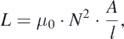
where μ0 is the magnetic constant, N the number of turns of the coil, A its cross-sectional area and l its length, we get

i.e. if a coil is enlarged by a factor of ten, the inductance increases tenfold.
With these results, we get for the decay time

The decay time of the RL circuit thus increases with the square of the scaling factor. Let us look at an example: we assume an RL circuit of laboratory size, with a linear dimension of about 0.1 m and a decay time of 1 millisecond. We do not even need a coil. Each closed circuit has an inductance and a resistance. We now imagine enlarging this circuit to 100 km, i.e. by a factor of 106. Equation (1) tells us, that the decay time will increase to 109 seconds or about 300 years. Closed currents on this scale thus remain practically constant for times of the order of 10 years. Significant changes are only observed in time intervals of the order of a hundred years.
We can transfer this result to the electric currents of the geodynamo. Due to the large size of the Earth, the decay time of an electric current within the outer core is of the order of years.
4.2. Conditions for a self-sustaining dynamo
In section 2, we have seen how a dynamo effect can occur in a moving, electrically conductive liquid. However, there is one problem we have not yet addressed. The dynamo effect cannot occur if the newly created field is smaller than the initial one. This would mean that the dynamo would extinguish. To prevent this happening, some conditions must be met.
One of these conditions is that the individual currents do not die away too quickly. Their decay time must be large. As we have seen, the decay time of a circuit is greater the larger its geometric dimensions are. Moreover, τ is great when the liquid is a good electrical conductor.
Furthermore, the functioning of the dynamo depends on the velocity of the liquid. Just like a technical dynamo, a geodynamo can only work when the velocity of the moving electrical conductors is sufficiently high.
So we have identified three parameters on which the functionality of the dynamo depends (i) the geometric extension l, (ii) the electrical conductivity σ and (iii) the velocity v of the liquid.
These three conditions are related in the simplest way one can imagine: the product of v, l and σ must reach a certain minimum value. Multiplying this product by the magnetic field constant μ0 results in a dimensionless quantity, called the magnetic Reynolds number:

The theoretical treatment of the problem shows that the minimum value for the occurrence of the dynamo effect is of the order of 10. However, for a geodynamo to run safely, Rm must even be larger.
For the Earth's outer core there is σ = 106 Ω−1 · m−1, v = 5 × 10⁻⁴ m s−1, and l = 1000 km.
With these values we obtain from equation (2) Rm = 1010, i.e. a value much greater than ten.
We can also understand why the effect does not show up in the bucket with the saltwater. With σ = 1 Ω−1 · m−1, v = 0.5 m s−1, and l = 0.2 m we get Rm = 10–7, a value that is far too small for a dynamo effect.
Somewhat more realistic would be the expectation that the movement of the water of the seas leads to a dynamo effect. Here a typical length would be about 100 m. But the magnetic Reynolds number is still far below the minimum value. So we should not be surprised that we do not encounter this effect anywhere on Earth except in the real geodynamo.
This seems to show that it is hopeless to realize a geodynamo effect in a laboratory experiment. However, such experiments have proved successful [9]. The facilities are several meters in size and work with liquid sodium, which is pumped to a speed of up to 20 m s−1. The path of the flowing sodium is predetermined. A magnetic Reynolds number of about 10 is achieved in these experiments.
5. The initial field
In order for our dynamo to start, a magnetic field B0 at the beginning is needed. Two remarks can be made about the origin of this field.
1. If an electrically conductive liquid moves sufficiently quickly and irregularly, the field-free state is unstable. The system assumes the dynamo state 'by itself'. 'By itself' means that a very small disturbance is sufficient to bring the system out of the field-free state. It is similar to a pencil that is placed on its tip. It tips over immediately, although there is a force-free state in which it would stand vertically. But hardly anyone will be surprised that it tips over anyway, and hardly anyone will ask why it falls in the direction in which it falls. Transferred to the geodynamo, this means: the question about the starting field is not interesting. It is an example of spontaneous symmetry breaking.
2. Whoever is not satisfied with this statement must engage in investigating the mechanisms by which small electric currents, and thus magnetic fields, originate (similar to the person who wants to predict the direction in which the pencil tips, for example, has to deal with air currents and other small effects). Electrochemical or thermoelectric processes can be considered. For both, the conditions are given. However, these small causes, which were responsible for the starting of the dynamo, are certainly more difficult to investigate than the functioning of the running dynamo, because one asks for effects that were effective under the conditions that prevailed several billion years ago.
6. Conclusion
Although we are far from being able to calculate the Earth's magnetic field and its evolution over time, we now know the functional principles of the geodynamo and the reasons for its strange behavior. Let us summarize them once again.
A dynamo effect occurs, when an electrically conductive fluid moves helically.
The larger a circuit, the slower the current decays.
The occurrence of the dynamo effect depends on
- the velocity of the flow;
- the electrical conductivity; and
- the geometric extension of the currents.
If the conditions for the occurrence of the dynamic effect are fulfilled, the currentless state is unstable.