


Abstract
The motion of a particle described by the Langevin equation with constant diffusion coefficient, time dependent linear force ( ) and periodic load force (
 ) is investigated. Analytical solutions for the probability density function (PDF) and n-moment are obtained and analysed. For
  the influence of the periodic term
  is negligible to the PDF and n-moment for any time; this result shows that the statistical averages such as n-moments and the PDF have no access to some information of the system. For small and intermediate values of
  the influence of the periodic term
  to the system is also analysed; in particular the system may present multiresonance. The solutions are obtained in a direct and pedagogical manner readily understandable by graduate students.
Export citation and abstract BibTeX RIS
1. Introduction
The Langevin equation is one of the fundamental equations for investigating non-equilibrium systems and it is significant to both theoretical and experimental processes. It has been extensively investigated and applied to diverse systems; many properties and analytical solutions of it have also been revealed, see for instance [1–5]. Besides, it has been largely employed to describe diffusion processes. The well-known example of a diffusion process is Brownian motion, and it can be described by using the Langevin equation or its corresponding Fokker–Planck equation. The diffusion processes are classified according to their mean-square displacements:

Anomalous diffusion has the mean-square displacement deviates from the linear time dependence; for  and
and  the system describes subdiffusion and superdiffusion, respectively. The well-established property of the normal diffusion described by the Gaussian distribution can be obtained by the usual Fokker–Planck equation with a constant diffusion coefficient (without the drift term) [1, 2], whereas anomalous diffusion regimes arise from a variable diffusion coefficient that depends on time and/or space [6–11]. Further, anomalous diffusion processes may arise from the chaotic dynamics [12, 13], aggregates of amphiphilic molecules [14], two-dimensional rotating flow [15], charge transport in amorphous semiconductors [16, 17], the dynamics of the bead in polymers [18], fast electrons in a hot plasma in the presence of dc electric field [19], turbulent two-particle diffusion in configuration space [20] and population growth models [21].
In this work a one-dimensional Langevin equation and its corresponding Fokker–Planck equation with constant diffusion coefficient, time dependent linear force and time dependent periodic load force are considered, and it is described by

where D is the diffusion constant and L(t) is the Langevin force given by

In order to maintain the harmonic potential the value of α is limited to  . The Fokker–Planck equation corresponding to the Langevin equation (2) is given by

where

are the drift and diffusion coefficients, respectively. The linear and load forces are important for investigating physical systems [4], i.e, the harmonic potential described by the linear force is a confining potential, whereas the load force conducts the particles of the system to its direction. A well-known example of a physical harmonic potential is the harmonic optical trapping potential, whereas a constant load force may be a constant electric field acting on charged particles. Besides, the load force has been used to describe multiple motors in biological systems (see [22] and the references therein). In particular, the Langevin equation with time dependent linear drift coefficient has been investigated in [23], and it can describe a wide class of anomalous diffusion processes. A complementary case of time-varying drift and diffusion coefficients has been considered in [24] to investigate turbulence. In many cases, the confinement of the atomic motions may be modelled by a linear force see for instance [21, 25, 26], i.e., a tagged particle trapped in a harmonic potential which describes the motion of all particles in the system such as the internal motions of proteins; in this case the periodic term  may be considered as an external force exerting on the system [27]. It can be shown that the system (4) may exhibit a stochastic resonance (SR) phenomenon by taking additional assumption. Conventional SR is related to a signal that can be boosted by adding noise to the signal, which contains a wide spectrum of frequencies. The frequencies in the noise corresponding to the original signal's frequencies will resonate with each other, amplifying the signal-to-noise ratio (SNR). Further, the SR may also be described by using other functions of the output signal, such as moments, autocorrelation and mean energy.
2. Results and discussions
The probability density function (PDF), n-moment and variance can be obtained from the Fokker–Planck equation (4) [28] and they are described by


and

where  is the variance given by


and

One can see that the function  given by equation (11) can determine the n-moment and variance. Moreover, it should be noted that the variance is a measure of the dispersion around the mean
  , and in the case of (10) it does not depend on the load force. However, the presence of the load force is important to the n-moment.
For the time independent linear force and constant diffusion coefficient ( and
and  ) the solution for the PDF, with the initial sharp condition

is given by [1]

For  (parabolic potential) the stationary state of the system exists; from the PDF (14) and considering large times yields

In the case of  (inverted parabolic potential) no stationary state exists, i.e, the PDF (14) goes to zero for
  .
.
Besides, the PDF (6) is peculiar, and it has the same solution of the time dependent linear force with the translation of the position coordinate (moving frame)

The translation of the position coordinate can also be demonstrated from the transformation of variable x in equation (4) [28].
It is interesting to note that for  the influence of the periodic term
  , with rapid oscillation, is negligible to the solution of the trajectory of the deterministic system, without the noise. This result is also extended to the system with the noise which can be seen from the PDF and n-moment for any time. It shows that the deterministic trajectory, statistical quantities such as n-moments and the PDF can not account for some information of the system. In the case of the periodic load force the first term on the right-hand side of equation (7) does not depend on the parameter Ω; the first term on the right-hand side of equation (8) does not also depend on the parameter Ω. Moreover, the integral of equation (7) can be solved analytically; first, it is written as follows:

Equation (17) can be integrated and the first moment in the limit  is given by

where
and In(z) is the modified Bessel function of the first kind [29]. Equation (18) can also be written as follows:

where

For  or
or  the first moment (21) reduces to [30]

with

It should be noted that the first moment (21) is written in terms of the periodic oscillation of the load force multiplying by a complicated coefficient which depends on the time, then the output amplitude gain G [31] can be determined and it is given by

The first moment (21) is equal to zero for  , without the periodic load force, in the limit
  . Without the periodic force in the linear force (
 ), the first moment is described by a simple behaviour given by equation (23). However, the presence of the periodic force
  may interact with the periodic load force and the system may present complicated behaviour for the n-moment. Figures 1–3 show the behaviours of the first moment (21). It may present strong oscillation for fixed times which depends on the parameter values
  and Ω. Figure 1 shows the tridimensional plot of the first moment in function of time and the parameter ω. The variation of the first moment is stronger for small values of ω. Figure 2 shows the tridimensional plot of the first moment in function of time and the parameter
  for small and large values of
  . For a fixed time one can see that the first moment presents strong interaction between the periodic force
  and periodic load force even for small values of
  . However, for large values of
  the first moment maintains a constant value for a fixed time, and the interaction between the two components disappears. Figure 3 shows tridimensional plot of the first moment in function of time and the parameter
  for small and intermediate values of
  one can see that the interaction between the periodic force
  and periodic load force is stronger for small values of
  , and it becomes weaker for larger values of
  . The numerical results plotted in figures 1–3 have been calculated from equations (7) and (21), and they are in good agreement. Thus, the numerical results for the gain G are also confident, and they are described below.
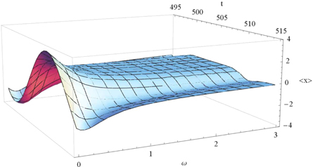
Figure 1. Tridimensional plot of the first moment  (21) versus ω and time t. The parameters are given by
  and
and  .
.
Download figure:
Standard image High-resolution image
Figure 2. Tridimensional plots of the first moment  (21) versus
  and time t. The parameters are given by
  and
and  .
.
Download figure:
Standard image High-resolution image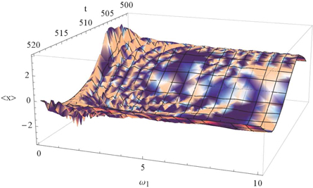
Figure 3. Tridimensional plot of the first moment  (21) versus
  and time t. The parameters are given by
  and
and  .
.
Download figure:
Standard image High-resolution imageFigures 4 and 5 show the behaviours of the output amplitude gain G and its dependence of the parameters ω and  . These figures show that the system presents a resonance phenomenon. In figure 4 the system shows a main peak for a fixed time near
  , whereas in figure 5 the system exhibits many peaks for a fixed time which corresponds to multiresonance [31]. The strong oscillation of the gain G is also present for small values of α (
 ), however the oscillation amplitude of this case is smaller than the case of
  . The oscillation amplitude also becomes smaller for larger values of
  .
.

Figure 4. Tridimensional plot of the gain G (25) versus ω and time t. The parameters are given by  and
and  .
.
Download figure:
Standard image High-resolution image
Figure 5. Tridimensional plots of the gain G (25) versus  and time t. From top to bottom correspond to the parameter
  and 0.95, respectively. The other parameters are
  and
and  .
.
Download figure:
Standard image High-resolution image
3. Conclusion
The SR phenomenon has been the subject of many investigations and it has been found in linear and nonlinear stochastic systems for single and collective particles. For linear systems driven by the additive white noise see for instance [32]; for nonlinear systems driven by the additive white noise see for instance [30, 32–35]; and for systems driven by multiplicative noise see for instance [31, 36–39]. For conventional SR the SNR versus the noise intensity exhibits a peak. In the wider sense of SR, certain functions of the output signal, such as moments, autocorrelation, mean energy [39] and SNR on the noise and system parameters exhibit non-monotonic behaviour [27]. Equation (4) is an overdamped linear system driven by the periodic load force and the additive white noise, and the system can describe multiresonance; the influence of noise can be included by taking additional assumption. Note that the results have been obtained in a direct and pedagogical manner readily understandable by graduate students.
Acknowledgments
The author acknowledges partial financial support from the Conselho Nacional de Desenvolvimento Científico e Tecnoló gico (CNPq), a Brazilian agency, under Grant No 301066/2015-9.