

Abstract
Elastic and inelastic interactions between optical spatial solitons in nonlinear optics, which to our knowledge have not been reported before, are investigated in this paper. Analytic soliton solutions for the coupled nonlinear Schrödinger equation are obtained using the Hirota method. The coefficient constraints, which can be used to determine whether the soliton interactions are elastic or inelastic, are presented. With different coefficient constraints, the characteristics of soliton interactions are exhibited. The results of this paper may have applications in the design of directional couplers and all-optical logical gates.
Export citation and abstract BibTeX RIS
1. Introduction
Since their theoretical prediction in 1973 and experimental demonstration in 1980 [1, 2], optical solitons have been the subject of intense theoretical and experimental studies in nonlinear optics [3–18]. In particular, optical spatial solitons, which exhibit the fascinating characteristics of self-guided beams, are an attractive and active area of research, because of their potential applications in many areas, including all-optical switching, optical data storage, distribution, and processing [19–28]. Intuitively, optical spatial solitons result from the interplay between diffraction and nonlinearly induced self-lensing or self-focusing effects [29].
Being nonlinear objects, optical spatial solitons can interact with each other. Interactions between optical spatial solitons can be classified into two categories: elastic and inelastic interactions [30]. For elastic interactions, optical spatial solitons are mechanical particles, the number of solitons is conserved, and the a single soliton recovers its initial trajectory and shape after interactions [31]. Furthermore, the elastic interaction system is integrable, no energy is transferred to radiation waves, and energy is conserved in each soliton [31]. For inelastic interactions, some solitons merge together or give birth to new solitons after interactions. The interaction progress is accompanied by energy dissipation, meaning a single soliton does not necessarily maintain its profile or identity [32]. Based on the properties of interactions, the application of optical spatial solitons in all-optical devices has been discussed extensively, including all-optical switching, wavelength auto-routers, and logic gates [33–36].
In this paper, interactions between optical spatial solitons will be investigated using the following coupled nonlinear Schrödinger (CNLS) equations [37–39]:


where q1(z,t) and q2(z,t)are the normalized envelopes of two modes. The subscripts z and t denote the partial derivatives with respect to the normalized distance and retarded time, respectively. σ1 and σ4 are the cross-coupling coefficients, and σ2 and σ3 are the self-coupling coefficients. The classical values of σ2 and σ3 are 1,2/3 and 2 [37, 38]. When σ1 = σ4 = 1/2 and σ2 = σ3 = β/2, with β as a real-valued constant, solitons in CNLS equations have been classified into infinite families [42]. When σ1 = σ4 =± 1 and σ2 = σ3 =± 1, bright and bright–dark type multi-soliton solutions of CNLS equations with focusing, defocusing and mixed type nonlinearities have been obtained using the Hirota method, and the interaction dynamics of solitons have been investigated [40, 41, 43, 19, 44–51]. Also, in [45], it was demonstrated that left- and right-handed (normal) nonlinear media have compound dark and bright solitons, respectively. When σ1 = σ4 = (1 − B)/2 and σ2 = σ3 = (1 + B)/2, as B = 1/3 in optical fibers, an analytic and numerical study has revealed the existence of a class of bound vector solitons in isotropic Kerr materials [52], and the properties of elliptically polarized solitons in isotropic optical fibers have been investigated [53]. Furthermore, a theory of acoustic vector solitons with self-induced transparency has been constructed with the appropriate values of σ1,σ2,σ3 and σ4 [54].
However, to the best of our knowledge, elastic and inelastic interactions have not been investigated comprehensively for equations (1) and (2) in the existing literature. In this paper, we will analyze the elastic and inelastic interactions between optical spatial solitons. According to the different coefficient constraints of σ1,σ2,σ3 and σ4 for equations (1) and (2), we will reveal the elastic or inelastic interactions in the same system, respectively. The influence of the corresponding parameters will be discussed to distinguish the elastic and inelastic interactions.
The structure of the present paper will be as follows. In section 2, the analytic soliton solutions for equations (1) and (2) will be derived using the Hirota method, and the parameter constraint relations will be obtained. In section 3, an asymptotic analysis will be made, and we will discuss the elastic and inelastic interactions between optical spatial solitons. Finally, our conclusions will be given in section 4.
2. Analytic soliton solutions for equations (1) and (2)
To derive the analytic soliton solutions for equations (1) and (2), the dependent variable transformations for equations (1) and (2) are introduced as follows [55],

where g(1)(z,t) and g(2)(z,t) are both complex differentiable functions, and f(z,t) is a real function. Considering the transformations (3), the partial derivative forms of q1(z,t) and q2(z,t) are given as
Here, Hirota's bilinear operators Dz and Dt [56] are defined by
Straightforward substitution of expressions (4) and (5) into equations (1) and (2) gives rise to the following equations,
where ∗ denotes the complex conjugate. Equations (7) and (8) can be rewritten as
Thus, the bilinear forms for equations (1) and (2) can be obtained as


Bilinear forms (11)–(14) can be solved by the following power series expansions for g(1)(z,t),g(2)(z,t) and f(z,t):


where ε is a formal expansion parameter. Substituting expressions (15)–(17) into bilinear forms (11)–(14) and then equating coefficients of the same powers of ε to zero yields the recursion relations for the  s,
s,  s and fn(z,t)s. Then, soliton solutions for equations (1) and (2) can be obtained. Firstly, we assume that

where θ1 = m z + k t = (m1 + i m2) z + (k1 + i k2) t, and θ2 = n z + w t = (n1 + i n2) z + (w1 + i w2) t. γ1, γ2, γ3, γ4, m1,m2,k1,k2,n1, n2,w1 and w2 are all real constants. Substituting  and
and  into bilinear forms (11)–(14), after some calculations, we can get the constraints on the parameters:

and
with
and the coefficient constraints

or

For the coefficient constraint (21),
For the coefficient constraint (22),


with
Without loss of generality, we set ε = 1, and the analytic soliton solutions can be expressed as
3. Discussion
With solutions (31) and (32), we will perform the asymptotic analysis, discuss interactions between optical spatial solitons with different coefficient constraints, and analyze the influence of the corresponding parameters for optical spatial soliton interactions.
3.1. Asymptotic analysis
(1) Before interactions (z → −∞).
(a)  :
:
(b)  :
:

(2) After interactions (z → +∞).
(a)  :
:
(b)  :
:

We can substitute the parameters A1,A2,B1,B2,B3, B4 and E1 into expressions (33)–(40), and then investigate the soliton interactions. Although equations (1) and (2) admit two-soliton solutions, soliton interactions in both of the coefficient constraints (21) and (22) are of different natures. Next, we will discuss the properties of soliton interactions with different coefficient constraints.
3.2. Elastic interactions with the coefficient constraint (21)
Under the condition of the coefficient constraint (21), and substituting expressions (23)–(25) into expressions (33)–(40), we can derive

Expressions (41) mean that the soliton interactions are elastic, as can be seen in figure 1. The optical spatial solitons simply pass through each other without radiation losses. They remain virtually unaffected when they interact with each other, and preserve their identities and form. That is to say, the amplitude, velocity and shape of optical spatial solitons undergo no changes after the interactions. The only effect of such interactions on optical spatial solitons is the phase shift. In addition, as long as the incidence angle of optical spatial solitons is not equal to zero, the trajectories and velocity of optical spatial solitons will be conserved, and optical spatial solitons will recover their initial values after interactions.
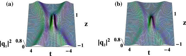
Figure 1. Elastic interactions between optical spatial solitons. Parameters are: k1 = 1, k2 =− 1, w1 = 1, w2 = 1, μ = 1, γ2 = 1, γ3 = 4, γ4 = 3, σ3 = 2, and σ4 = 3.
Download figure:
Standard image High-resolution imageHowever, if the interactions occur at zero angular separation between optical spatial solitons, they will form a bound pair. As shown in figure 2, the parameters are the same as those given in figure 1, but with k1 = 1.5,k2 =− 0.1,w1 = 2, and w2 =− 0.1, the incidence angle between the solitons is zero, and bound solitons appear, revealing an oscillatory motion. The optical spatial solitons combine and separate periodically during their propagation. Figure 3 is the contour plot of figures 1 and 2. Thus, the interactions are mainly governed by the interaction angle of the optical spatial solitons in this case.
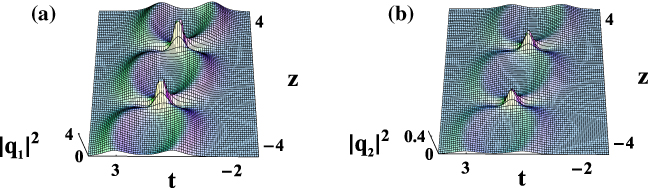
Figure 2. Elastic interactions between optical spatial solitons with the same parameters as those given in figure 1, but with k1 = 1.5,k2 =− 0.1,w1 = 2, and w2 =− 0.1.
Download figure:
Standard image High-resolution image
Download figure:
Standard image High-resolution image3.3. Inelastic interactions with the coefficient constraint (22)
Substituting expressions (26)–(30) into expressions (33)–(40), we can obtain that

According to expressions (42), we can find that the soliton interactions are inelastic in figure 4. That is, there is an energy exchange between optical spatial solitons after interactions. Figure 5 is the contour plot of figure 4. As shown in figures 4 and 5, inelastic interactions can result in energy exchange, where energy can be lost or transferred from one soliton to another.
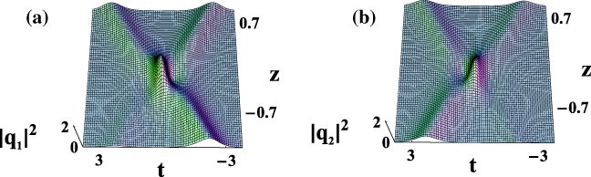
Figure 4. Inelastic interactions between optical spatial solitons. Parameters are: k1 = 1.5, k2 =− 1, w1 =− 1.5, w2 = 1, μ = 1, γ1 = 1, γ2 = 2, γ3 = 3, γ4 = 1, σ3 = 2, and σ4 = 3.
Download figure:
Standard image High-resolution image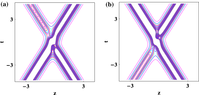
Download figure:
Standard image High-resolution imageSimilar to figure 2, when the interactions occur at zero angular separation between optical spatial solitons, then bound solitons can also be obtained, as shown in figures 6 and 7. The difference is that energy exchanges periodically. That feature can give rise to new phenomena, such as merging of optical spatial solitons. Therefore, inelastic interactions are attractive for guiding, directing and manipulating solitons with other solitons without any intervening fabricated structures.
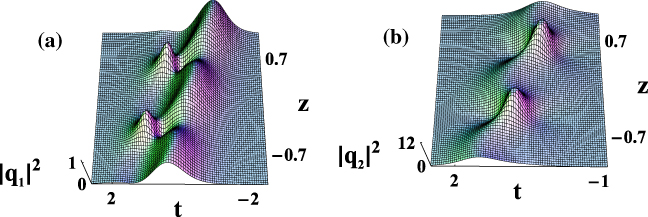
Figure 6. Inelastic interactions between optical spatial solitons. Parameters are: k1 = 1.5, k2 =− 0.3, w1 = 3, w2 =− 0.3, μ = 1, γ1 = 3, γ2 = 2, γ3 = 1.5, γ4 = 3, σ3 = 2, and ma4 = 1.
Download figure:
Standard image High-resolution image
Download figure:
Standard image High-resolution image
4. Conclusions
In conclusion, we have investigated elastic and inelastic interactions between optical spatial solitons in nonlinear optics. With symbolic computation, the coupled nonlinear Schrödinger equation (see equations (1) and (2)) has been studied analytically, and the analytic soliton solutions (31) and (32) for equations (1) and (2) have been obtained with two coefficient constraints (21) and (22); this being the key point of this paper. According to the two coefficient constraints, we have conducted an asymptotic analysis and demonstrated elastic and inelastic interactions respectively. For elastic interactions (see figures 1 and 2), the trajectories and velocity of optical spatial solitons were conserved, and optical spatial solitons recovered to their initial values after interactions. Inelastic interactions resulted in energy exchange, with energy being transferred from one soliton to another (see figures 4 and 6). The results of this paper have potential applications in all-optical switching, distribution, and processing.
Acknowledgments
This work has been supported by the National Natural Science Foundation of China under Grant No. 61205064, by the Fundamental Research Funds for the Central Universities of China (Grant No. 2012RC0706), and by the National Basic Research Program of China (Grant No. 2010CB923200).