Abstract
Bone mineral density at spine and hip is widely used to diagnose osteoporosis. Certain conditions cause changes in bone density at other sites, particularly in the lower limb, with fractures occurring in non-classical locations. Bone density changes at these sites would be of interest for diagnosis and treatment. We describe an application, based on an existing software option for Hologic scanners, which allows reproducible measurement of bone density at six lower limb sites (upper femur, mid-femur, lower femur; upper leg, mid-leg, lower leg). In 30 unselected subjects, referred for bone density, precision (CV%) measured on 2 occasions, separated by repositioning, ranged from 1.7% (mid-femur) to 4.5% at the lowest leg site. Intra-operator precision, measured by three operators on ten subjects on three occasions, was between 1.0% and 2.9%, whilst inter-operator precision was between 1.0% and 3.6%, according to region. These values compare well with those at the spine and upper femur, and in the literature. There was no evidence that this operator agreement improved between occasions 1 and 3. This technique promises to be useful for assessing bone changes at vulnerable sites in the lower limb, in diverse pathological states and in assessing response to treatment.
Export citation and abstract BibTeX RIS
For more information on this article, see medicalphysicsweb.org
Introduction
Bone mineral density (BMD) measurements at the spine or upper femur are widely used to help determine fracture risk of osteoporosis (Cummings et al 1994), in evaluating the response to treatment (Cummings et al 1998) and may also be a determinant of quality of life (Wilson et al 2012).
Under some circumstances, localized changes in BMD lead to increased fracture risk at specific skeletal sites, not necessarily reflected by spine and upper femur BMD measurements. For example, patients with stroke have an increased risk of fracture in the lower limbs (Davie et al 2003, Haddaway and Davie 2008), and fractures at the lower end of the femur and upper tibia (Comarr et al 1962, Ragnarsson and Sell 1981) in spinal cord injury (SCI) stress the importance of measuring bone loss at sites other than those classically assessed by dual x-ray absorptiometry (DXA) (Chow et al 1996). Modern advances in patient management have led to the prospect of walking in patients with SCI, leading to greater interest in the integrity of bone at sites in the lower limb and the need to examine whether drug or other therapies can reverse bone loss, at those sites especially at risk of fracture.
Not only is bone loss of interest, but, under certain circumstances, increased bone density at particular locations may also be of interest. Use of antiresorptive drugs, particularly the bisphosphonates (Giusti et al 2010), is associated with 'atypical' fractures occurring in the femur, from below the lesser trochanter to mid-shaft. Many reports comment on the increased cortical thickness found on the non-fracture side in patients with 'atypical' femoral fractures (Lenart et al 2008, Shane et al 2010). The ability to identify patients with unusually dense bone in the mid-femur might aid clinical decision making about whether to commence, continue or discontinue treatment.
Since DXA is, by definition, an 'areal' measurement, combining both cortical and trabecular bone, techniques which isolate areas of predominantly one type of bone (such as in QCT) can be valuable. Briggs et al (2010) has combined the use of sub-regions and scanning of the lateral lumbar spine, to assess the predominantly trabecular fraction of the spine.
Previous reports, using bone densitometry to obtain measurements of largely trabecular bone around the knee, have used various methods. Biering-Sorenson (Biering-Sørensen et al 1988) reported a relationship between bone mineral content and the presence of fracture in the lower extremities, in SCI patients. The more successful of these methods have applied the DXA lumbar spine analysis protocol to obtain measurements around the lower femur and upper tibia in SCI adults (Bloomfield et al 1996, Shields et al 2005), SCI children (Lauer et al 2007) and in osteoarthritis (Beattie et al 2005). However, use of this protocol for limbs can lead to incorrect application of the bone edge algorithm in the absence of sufficient soft tissue within the region (Murphy et al 2001).
The application described in this paper exploits the whole body facility of the Hologic QDR4500A, which allows a rapid acquisition of lower limb data without the patient having to be manipulated and without relying on external measurements. We have used an existing Hologic sub-regional analysis option to collect data from six well defined regions in the lower limb, to include the femur and tibia/fibula. The use of this option has been applied elsewhere in the analysis of bone changes in post-operative total hip replacements, for the measurement of Gruen Zones (Albanese et al 2009), for regions around the knee in inflammatory arthritis (Murphy et al 2001) and in SCI (Garland et al 2001). Lunar DXA machines have applied sub-regions to measure BMD in the knee (Vazquez et al 2004, Soininvaara et al 2004).
Materials and methods
Thirty consecutive patients (mean age: male (n = 3), 67 year; female (n = 27), 63 year), presenting for DXA scanning, were recruited from the Bone Metabolism unit at the Robert Jones and Agnes Hunt Orthopaedic Hospital as part of a (larger) service evaluation to measure scan precision, on a Hologic QDR4500A scanner (including hip, spine and whole body), following machine change and software upgrades.
The Local Research Ethics Committee was consulted and advised that submission was unnecessary for a service evaluation, provided appropriate patient information and consent were undertaken, which took place subsequently.
The software version was APEX 3.3. Patients presented for bone density assessment for osteoporosis. Regular quality control, including whole body tests, is performed routinely as per the manufacturer's requirement. Each patient underwent a whole body DXA scan, which was then repeated after the patient had got off and then back onto the scanning couch to evaluate re-positioning errors. This set of patient scans was used to undertake the lower limb analysis (LLA) in this study, using the manufacturer's 'sub-region analysis' programme, and to evaluate its precision with regard to re-positioning error. A sub-set of ten subjects, was analysed three times, by three different operators (HLD, CAS, MJH), to measure the inter- and intra-operator variation of the LLA technique.
Intra-operator coefficient of variation (CV) was calculated from the three measurements of each subject by each operator. Inter-operator CV was obtained from the first set of results obtained by each operator and from the third set of results. The results obtained from the third analysis were compared with the results from the first to investigate whether there might be a learning curve.
It is necessary to undertake a routine whole body analysis, prior to sub-region analysis, according to the conventional manufacturer protocol. In sub-region analysis mode, 6 regions (R1 to R6), covering each lower limb (hip to ankle, left and right, giving a total of 12 regions), were generated (see figure 1 and appendix).

Figure 1. Illustrating the six manually defined sub-regions (R1–R6) within the lower right leg used to acquire sub-regional BMD. Note that all boxes are extended to include air also allowing analysis of body composition indices (data not reported).
Download figure:
Standard image High-resolution imageThe right femur and tibia/fibula (subsequently referred to as tibia) were each sub-divided into three regions (femur: R1 (region 1) to R3 (region 3); tibia: R4 to R6), wherever possible of equal length, with the lower margin of R3 and the upper margin of R4 passing through the knee joint space. Further adjustment was sometimes required, to produce regions of equal size. Where this was necessary, lines were added to, or subtracted from, R1 or R6.
Region R1 was truncated at its superior, medial corner, to avoid inclusion of the ischium. R6 is adjusted to include the tibia, but not the foot. Regions were selected to include air as well as tissue for the purpose of assessing body composition at the same time (results not reported here).
To analyse the left leg, the right lower limb regions were 'mirrored' to outline the left limb regions. It was sometimes necessary to further adjust the regions at this point.
Statistics
Precision and inter- and intra-observer variation, for analysis of lower limb, were calculated using the International Society of Clinical Densitometry (ISCD) calculator (ISCD 2013), to give root mean square coefficient of variation. For the purpose of this paper, BMD has been used in each case. Least significant change (LSC), that value representing the smallest change in BMD considered biologically significant on the basis of measured CV (=2.77 × CV), was derived from the precision results (Baim et al 2005). The number in parenthesis (2.77) represents the 95% confidence interval (CI) associated with the value  .
.
ANOVA was used to test for statistically significant differences in precision, between the different regions of interest, and to test for the presence of a learning curve in the intra-operator data, by comparing the first and the third set of analyses. Precision results for left and right lower limbs were compared with the paired t-test.
Agreement between operators, within operators and investigation of any 'learning' effect on repeatability (differences between earlier (first) and later (third) analyses), was also calculated using intraclass correlation coefficients (ICC) (SPSS v18). The ICC is designated as ≤ 0.40: poor to fair agreement, 0.41–0.60: moderate agreement, 0.61–0.80: good agreement, and 0.81–1.00: excellent agreement (Bartko 1966).
Results
As a measure of machine and protocol repeatability the coefficients of variation (CV%) for the 30 subjects for BMD, at the 6 regions designated for the right lower limb, are shown in table 1. Data are presented as percentage (CV%) and also as a root mean square standard deviation (RMS SD) in gm cm−2. Values ranged from 1.7 to 4.5%, with the lowest being at the mid- and lower sites in the femur. These results demonstrate the greater difficulty in repeating analyses at regions R1 and R6, those areas close to the hip and the ankle, respectively, and also appear to show R5 (mid-tibia) to be less consistent than R2 (mid-femur).
Table 1. Machine precision (obtained from 30 subjects) as coefficient of variation (%CV), and least significant change (%LSC) for lower limb sub-regional data acquisition. Also included are absolute RMS SD expressed in terms of gm cm−2.
| Machine precision for right lower limb BMD | ||||||
|---|---|---|---|---|---|---|
| Sub-region | R1 | R2 | R3 | R4 | R5 | R6 |
| % CV | 3.5 | 1.7 | 2.6 | 2.6 | 4.2 | 4.5 |
| RMS SD (gm cm−2) | 0.039 | 0.026 | 0.026 | 0.023 | 0.048 | 0.034 |
| %LSC | 9.8 | 4.6 | 7.1 | 7.2 | 11.5 | 12.4 |
| LSC (gm cm−2) | 0.11 | 0.07 | 0.07 | 0.06 | 0.13 | 0.09 |
Acquisition (CV%) errors at R3 and R4, the regions representing the distal femoral and proximal tibial condyles around the knee, comprising greater proportions of cancellous bone, are similar (2.5–2.6%) with LSC values in the range 7.1–7.2% indicating that changes of approximately 7.2% (or more) would imply a clinically or biologically meaningful change in BMD from a baseline or reference value (table 1).
Analysis was also performed on the data derived from the left lower limb. Comparison of left and right lower limbs revealed no significant differences in repeatability and these data are not reported.
Intra-operator variability, for the right lower limb only, as a measure of an individual operator's precision at repeating the same analysis, shows good agreement (table 2). ANOVA on these results revealed no significant difference between operators.
Table 2. Intra-operator and inter-operator errors (obtained from a subset of ten subjects) in the analysis of the sub-regions of the lower limb (values are CV%).
| Operator error for right lower limb BMD (%CV) | ||||||
|---|---|---|---|---|---|---|
| Sub-region | R1 | R2 | R3 | R4 | R5 | R6 |
| Intra-operator | ||||||
| MJH | 2.3 | 1.5 | 1.6 | 1.0 | 0.7 | 2.9 |
| CAS | 2.0 | 1.5 | 1.3 | 1.1 | 1.4 | 2.5 |
| HLD | 2.0 | 1.3 | 1.4 | 1.1 | 1.5 | 2.6 |
| Inter-operator | ||||||
| First meas. | 3.5 | 1.4 | 1.4 | 1.1 | 1.2 | 2.5 |
| Third meas. | 1.6 | 1.0 | 1.3 | 1.5 | 1.7 | 3.6 |
Inter-operator variability is also shown in table 2. This indicates that not only are the individual operators achieving good precision with this protocol, but that agreement between operators is robust. Comparison between the first and the third measurement did not show statistically significant evidence of a learning effect. Values of ICC also support the conclusion that results do not appear different for first or third analysis (table 3).
Table 3. Intra-class correlation coefficient (ICC (95% CI)).
| Intra-operator (ICC (95% CI)) | ||||||
|---|---|---|---|---|---|---|
| Rater | R1 | R2 | R3 | R4 | R5 | R6 |
| MH | 0.979 (0.941; 0.994) | 0.996 (0.990; 0.999) | 0.997 (0.991; 0.999) | 0.998 (0.993; 0.999) | 0.999 (0.997; 1.000) | 0.986 (0.961; 0.996) |
| CS | 0.988 (0.967; 0.997) | 0.996 (0.988; 0.999) | 0.997 (0.991; 0.999) | 0.996 (0.989; 0.999) | 0.996 (0.988; 0.999) | 0.990 (0.971; 0.997) |
| HD | 0.990 (0.973; 0.997) | 0.997 (0.989; 0.999) | 0.997 (0.988; 0.999) | 0.996 (0.987; 0.999) | 0.996 (0.987; 0.999) | 0.994 (0.982; 0.998) |
| Inter-operator | ||||||
| First analysis | 0.970 (0.918; 0.992) | 0.996 (0.989; 0.999) | 0.997 (0.992; 0.999) | 0.997 (0.991; 0.999) | 0.996 (0.990; 0.999) | 0.991 (0.972; 0.997) |
| Third analysis | 0.992 (0.978; 0.998) | 0.998 (0.994; 0.999) | 0.998 (0.994; 0.999) | 0.994 (0.979; 0.998) | 0.996 (0.988; 0.999) | 0.983 (0.948; 0.996) |
Discussion
We have described a novel application for the analysis of the BMD in defined regions of the lower limb, obtained from whole body DXA scans, and tested the related machine and operator precision. Machine precision or repeatability with patient repositioning ranged from 1.7% (R2) to 4.5% (R6). This compares well with the study by Albanese et al (2009) using this analysis option in hip prostheses, which reported precision ranging from 1.5 to 3.7%. Our poorest precision was at R1 and R6, around the hip and ankle respectively. These regions are most subject to variation in patient position and are also those used for the finer adjustments within the protocol, when the upper or lower leg did not divide exactly into three. The exception to this was at R5 (mid-tibia). We investigated the possible causes of this higher value. It was not found to be a result of overlap of the tibia and fibula bones, nor a result of poor positioning of the region of interest in this case. One possibility is that the relative contribution of cortical and trabecular bone may vary between patients at this site. The study by Murphy et al (2001) found better precision at the femur compared with the tibia. Soininvaara et al (2004), using a Lunar machine, found an average precision of 2.5% at the knee.
The values for precision at R2–R4 compare well with those for conventional DXA hip and spine precision, measured on the same sample of patients, of 1.8% (lumbar spine), 1.1% (total hip) and 1.9% (femoral neck), and for those reported in a lateral in vivo spine study by Briggs (Briggs et al 2005).
The minimum acceptable precision recommended by the ISCD (ISCD 2012) for these regions measured by DXA is 1.9% (LSC = 5.3%), 1.8% (LSC = 5.0%) and 2.5% (LSC = 6.9%) respectively, which relate to machine precision for an individual operator. These values do not specifically apply to inter- and intra-operator precision, but our values concur with those reported by Briggs in cadavers (Briggs et al 2010) and in patients (Briggs et al 2005).
Our results include the ICC for inter- and intra-operator precision showing that the protocol is robust for regions R2 through R5 (mid-femur to mid-tibia). These ICC results are comparable with lumbar spine analysis agreement figures from Briggs et al (2005).
There was no evidence from our study that observer agreement improved with repeated analyses.
The novel application described here is based on a standard whole body DXA scan and does not require any special acquisition parameters or additional radiation dose compared with a conventional DXA whole body scan. Although not included here, it is also possible to extract body composition data for these sub-regions. Our technique enables regional information to be obtained in those disease conditions which affect the lower limb, such as bone loss following neurological damage, as in SCI and stroke. It also enables a degree of differentiation between sites at which cortical (e.g. mid-femur) or trabecular (e.g. lower femur or upper tibia) bone predominate, thereby giving information about changes affecting different types of bone. The potential to provide information relating to changes of bone mass within these bony fractions may prove clinically useful. However, this information is still a function of areal BMD and lacks the cross-sectional information available from peripheral QCT.
At this time, healthy reference data for the lower limb regions are not available for this technique. Thus z- and t-scores are not available. However, with the proviso that the expected bone loss will exceed the LSC at these sites, this application may prove useful in monitoring longitudinal changes of BMD in the lower limbs, particularly at those sites known to be at increased risk of fracture, such as around the knee in SCI patients.
Bone densitometry is now widely available, although the full technological potential of the densitometers is not widely exploited. The application described here can be simply performed on a whole body DXA scan with minimal radiation exposure (whole body scans take 5 min with a radiation dose of 4.2 microSieverts, (effective dose) to the patient. Application to the upper limb, as well as to body composition for both upper and lower limb, could also be assessed using this technique.
Several limitations to this application are acknowledged. Firstly, the method has been developed only for a Hologic fan beam densitometer and we are not able to comment on how it might be adapted to DXA scanners from other manufacturers, or to older pencil beam devices. Secondly, we have assessed precision of the technique on a relatively able and compliant patient sample, and data are derived from this particular scanning centre. Patient groups in which this technique could be valuable include subjects in whom positioning errors may be more confounding and where movement artefacts might be more prominent, although this can also apply to other conventional scanning sites as well. As such, the true repeatability errors may be greater in other patient groups. In the study by Briggs et al (2005) a greater imprecision was reported for an elderly cohort of patients, compared with a younger study group.
Whilst hip and spine regions are considered the gold standard for DXA scanning in those populations where the pathological process is 'homogeneous' or systemic, these sites may be less useful where immobility or neurological damage affects specific anatomical sites. The use of lower limb DXA analysis could extend the application of bone densitometry in these, and other, populations.
Acknowledgment
We wish to acknowledge the assistance of Gwyneth Williams (radiographer) who participated in the initial development of this technique.
Appendix:
Appendix. Whole body: lower limb analysis protocol
- (1)The whole body scan will have been acquired and analysed, according to the recommendations in the relevant Hologic manual.
- (2)Enter sub-region analysis mode. Adjust grey scale, if necessary, to show soft tissue, necessary if 'Body Composition Analysis' (BCA) is required.
- (3)Display lower limbs.
- (4)Select '+' to display first region R1 (figure 2).
- (5)With 'Whole Mode' selected on the left hand menu, move yellow box, so that its top left hand corner is above, and to the left of, the greater trochanter, with its lateral border in air.
- (6)Select 'Line Mode' and drag bottom edge (selected line becomes 'broken') so that it passes through the knee joint space. Keyboard arrow keys may be used for finer adjustment of position. (NB: it is necessary to select a box/line/point with the mouse before using the keyboard arrows.) Both lateral borders should be positioned in air, the medial normally corresponding to patient midline.
- (7)Dimensions of the region are displayed below the image. (Note that the higher number is not necessarily the longer dimension.)
- (8)Add 2 to the box length before dividing by 3 (to allow for line thickness). The femur will be divided up into three regions equal in length (e.g. if length + 2 = 36, each box will need to be 12). If it is not divisible by 3, allocate the extra line or two to the upper region (which will be R1). E.g. if length + 2 = 35, then R1 = 13, R2 = 11 and R3 = 11. Move the distal border up to the correct length, In this case 12. This is R1.
- (9)Click on 'Whole mode' and then click the '+' button and a new box appears.
- (10)Move this box (with an interrupted border), R2, to be in contact with, but not overlapping, the distal border of R1.
- (11)Adjust box borders as required, using 'Line mode' as appropriate (see below **), reducing the length if this box is to be smaller than R1. It is not necessary to move the lateral box border if it is still in air.** Ensure side borders of regions are in air, in order for body composition to be assessed, if required (it may be necessary to adjust the grey scale of the image to achieve this—see previously—step 3) except medial border of R1 and proximity of hand soft tissue.
- (12)This creates R2 and is the method for generating further regions.
- (13)Repeat for R3, with distal border passing through the knee joint space.
- (14)The end result should be that the individual boxes (regions) are equal in length if possible, but the extra line or two allocated to R1 if not (in this example, R1 = 12, R2 = 11, R3 = 11).
- (15)Having completed regions R1–R3, in 'Whole Mode' click on R1 to select it and then 'Point Mode'.
- (16)Move the upper medial corner point toward the left (using the keyboard arrow keys) until the line bisects the femoral neck. Ideally this line will miss the ischium, but this will not always be the case.
- (17)This completes the regions for the femur.
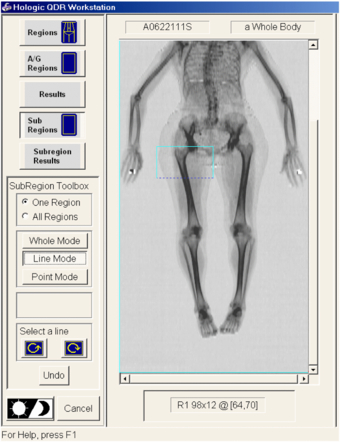
Figure 2. Selection of first region, R1.
Download figure:
Standard image High-resolution imageAppendix. For the tibia and fibula
- (18)Click on 'Whole Mode' and select R3.
- (19)Clicking on the (+) box will then generate a new box. Size this box to extend from the knee joint space to the distal tip of the fibula, using 'Line Mode' as appropriate to move the distal margin. Ensure lateral and medial margins are in air.
- (20)Divide and choose region lengths (adding 2 lines to the displayed length. e.g. (30 + 2) = 10 + 10 + 12), for R4 to R6, as for the femur. Adjust the length of R4, using 'Line Mode'
- (21)Ensure lateral borders are in air.
- (22)Click 'Whole mode' and then '+' button. Move box R5, to be in contact with, but not overlapping, distal border of R4.
- (23)Adjust the side borders as required, using 'Line mode' as appropriate (see above **). This creates the second region R5 and is the method for generating further regions.
- (24)Again click '+' sign, under 'Whole Mode', and repeat for R6, with distal border tangential to the distal tip of the fibula.
- (25)The end result should be that they are equal in length if possible, but the extra line or two allocated to R6 if not (in this example, R4 = 12, R5 = 11, R6 = 11).
- (26)With R6 selected, use 'Point mode', to select the distal medial corner of R6 and move upward until distal border of R6 is in line with distal end of medial malleolus. It may be necessary to move in the lateral border as well. Angle the distal border of R6 as necessary to run tangential to the distal fibula.NB: The proximal femur region (R1) region, and the ankle region (R6), are the most difficult to define and the operator should take care with these regions.
- (27)
- (28)If BCA is required then click on the BCA button.
- (29)To analyse the left lower limb, click sub-region button.
- (30)Select 'All Regions' on the 'Sub-region Toolbox' window, scroll down for lower limb, and then use double horizontal arrow (↔) bottom left to move the sub-regions over to the left limb, mirroring the positions on the right limb.
- (31)Remember at this point that the mirroring of the regions is about the centre of the scan field, not necessarily the centre line of the patient (unless they are positioned exactly in the centre).
- (32)Select each region in turn using arrows to adjust, if necessary.
- (33)Adjustment of sub-regions may be required, if limb length or position is unequal, but attempt to mirror position on both limbs as closely as possible.
- (34)Click to generate the report for the left leg. (Note that the regions will be labelled R1 to R6, since the 'R' stands for region not 'right'.)In cases where lower limbs are of unequal length, adjust the lower border of R3 for small differences. For large discrepancies, redraw regions again.

Figure 3. Final analysis results for all six regions.
Download figure:
Standard image High-resolution image