


Abstract
The effects of including the singlet metastable molecule O2(b ) in the discharge model of a capacitively coupled rf driven oxygen discharge are explored. We furthermore examine the addition of energy-dependent secondary electron emission yields from the electrodes to the discharge model. The one-dimensional object-oriented particle-in-cell Monte Carlo collision code oopd1 is used for this purpose, with the oxygen discharge model considering the species
  ,
,  ,
,  , O(3P), O(1D),
  , O+, O−, and electrons. The effects on particle density profiles, the electron heating rate profile, the electron energy probability function and the sheath width are explored including and excluding the metastable oxygen molecules and secondary electron emission. Earlier we have demonstrated that adding the metastable O2(a
 ) to the discharge model changes the electron heating from having contributions from both bulk and sheath heating to being dominated by sheath heating for pressures above 50 mTorr. We find that including the metastable O2(b
 ) further decreases the ohmic heating and the effective electron temperature in the bulk region. The effective electron temperature in the electronegative core is found to be less than 1 eV in the pressure range 50–200 mTorr which agrees with recent experimental findings. Furthermore, we find that including an energy-dependent secondary electron emission yield for
  -ions has a significant influence on the discharge properties, including decreased sheath width.
Export citation and abstract BibTeX RIS
1. Introduction
The capacitively coupled plasma (CCP) discharge plays a significant role in modern plasma processing technologies. Applying a radio-frequency (rf) current or voltage to the electrodes can sustain such discharges at low pressure, with a high-voltage sheath forming between the plasma bulk and the electrodes. The two main heating mechanisms for electrons in these discharges are electron-neutral collisions, which lead to ohmic (or collisional) heating in the bulk and sheath regions, and momentum transfer due to the moving sheaths which leads to stochastic (or collisionless) heating at the plasma edge, independent of the neutral density [1, 2]. In addition there can be an energy transfer as electrons flow across ambipolar fields towards the electrodes, representing a negative power absorption [3]. In an earlier study using the oopd1 particle-in-cell Monte Carlo collision (PIC/MCC) code we found that detachment by the metastable molecule O2(a ) has a significant influence on the discharge properties such as the electronegativity, the effective electron temperature, and the electron heating processes [4]. In a subsequent study we explored the evolution of the charged particle density profiles, electron heating mechanism and the electron energy probability function (EEPF) in a capacitively coupled oxygen discharge in the pressure range 10–500 mTorr [5]. We found that at higher pressures (50–500 mTorr) the electron heating occurs mainly in the sheath region and at low pressures (10 mTorr) ohmic heating in the bulk plasma (the electronegative core) dominates. Thus at low pressures the EEPF is convex, and as the pressure is increased the number of low energy electrons increases, the number of higher energy electrons (>10 eV) decreases and the EEPF develops a concave shape or becomes bi-Maxwellian. This contradicts what has been observed both experimentally [6] and by PIC/MCC simulations [7] in argon CCP discharges where stochastic heating dominates at low pressure and the role of ohmic heating increases with increased pressure. Thus in argon, the EEPF evolves from concave shape to convex shape as pressure is increased.
Since oxygen is a weakly electronegative gas, the ion concentration in the discharge is at most only a few times larger than the electron density. The oxygen chemistry is rather involved, due to the presence of metastable molecular and atomic oxygen and their interactions, including dissociative attachment and detachment processes. In particular, the two low lying singlet metastable states of the molecular oxygen, designated by a and b
and b , which are located 0.98 and 1.627 eV above the ground state X
 , respectively, can play a significant role in the overall chemistry. The a
 state can be produced in significant amount due to its stability against deactivation by collisions with other molecules and chamber walls, while the b
 state is less stable towards wall quenching but is effectively produced by energy transfer from the metastable atom O(1D) [8]. Decades ago it was pointed out by Thompson [9] that detachment by the b
 state may be a significant detachment process in the oxygen discharge. Global model studies of high density oxygen discharges, such as the inductively coupled discharge, indeed indicate that a significant fraction of the oxygen molecules are in the singlet metastable states a
 and b
and b [8, 10, 11]. Furthermore, these models indicate that both the metastable states have a significant contribution to the creation, through dissociative attachment, and destruction, through detachment, of the negative ion O−. These two low-lying excited electronic states of oxygen, a
 and b
and b , are also of considerable interest since they play important roles in the chemistry of the upper atmosphere [12]. This is due to the selection rules that prohibit their radiative and collisional transitions, such that they have very long lifetimes in the atmosphere. Both these states possess approximately the same nuclear separation and similarly shaped potential curves as the ground state X
 [13].
[13].
To date, ion-induced secondary electron emission yield implemented in PIC/MCC codes has usually been taken to be a constant, with the constant generally set to 0 or 0.2 for oxygen as bombarding species [4, 5, 14]. Roberto et al [15] explored the effects of varying a constant secondary electron emission yield in a 13.56 MHz capacitively coupled oxygen discharge simulated using xpdp1 (plasma device planar in 1 dimension for X windows), at a peak voltage of 500 V and pressure values of 20 and 200 mTorr, and found that as the secondary electron emission yield is varied from 0 to 0.4, the density profiles, electron energy distribution functions (EEDFs), and the electron heating rate profiles change significantly. Specifically, the electron density increases with increasing secondary electron emission yield at the higher pressure value of 200 mTorr. More recently, Derzsi et al [16] explored the effects of including an energy-dependent ion- and neutral-induced secondary electron emission yield in a 13.56 Mz argon discharge, in the pressure range 40–750 mTorr and voltage range 100–1000 V. They found that this changes the discharge characteristics significantly. With a realistic inclusion of heavy particles in the simulation, the plasma density and the ion flux towards the electrodes increases, and the sheath width decreases. For the energy-dependent secondary electron emission yields, they used fits developed by Phelps et al [17, 18], which were based on measurements from various metal surfaces for ion- and neutral-induced secondary electron yield due to argon bombardment.
The code oopd1 (object oriented plasma device in 1 dimension) used here is a 1d-3v object-oriented PIC/MCC code [19, 20], i.e. the model system contains one spatial dimension and three velocity components, and is an upgrade from the well known xpdp1 code [14]. The oxygen discharge model in the xpdp1 code only contained the species O2(X ,
,  -ions, O−-ions and electrons [21]. In the oopd1 code, we have added oxygen atoms in the ground state O(3P), O+ -ions, the molecular metastable O2(a
 ) and the metastable atom O(1D), along with revising all cross sections [4, 14]. Contrary to what has been done before, the metastables in oopd1 are not taken to be a constant fraction of the O2 density [22], they are both created and destroyed, and can be tracked kinetically.
Here we discuss the addition of O2(b ) to the reaction set and the effects of including energy dependent secondary electron emission yields for both oxygen ion (
 and O+) and neutral (O2 and O) bombardment of the electrodes. The reactions added and the cross sections used for O2(b
 ) are discussed in section 2. In section 3 we review measurements of the secondary electron emission yield for clean and oxidized metal surfaces by O+-ions,
  -ions, O atoms and O2 molecules and develop fits for the energy-dependent secondary electron emission yields. The cases explored are defined in section 4 and the results are compared and discussed in section 5. In section 5 we also compare the findings of the simulations to experimental observations. Concluding remarks are given in section 6.
2. Reactions involving the metastable O2(b )
)

The basic reaction set and cross sections included in the oopd1 code for the oxygen discharge are discussed in an earlier work [14] and will not be repeated here. Similarly, the reactions involving the metastable oxygen atom O(1D) and the metastable oxygen molecule O2(a ) are discussed elsewhere [4]. The most important reactions involving the metastable singlet molecule O2(b
 , as determined by a global model [8], are added to the discharge model and listed in table 1.
Table 1. The reaction set for oxygen reactions involving metastable oxygen molecule O2(b ).
).
| Reaction | Process | Reference |
|---|---|---|
e + O2(b ) → ) →  + e + e + e + e |
Ionization | Threshold reduced |
e + O2(b ) → O(3P) + O− ) → O(3P) + O− |
Dissociative attachment | Threshold reduced from  [23] [23] |
e + O2(b ) → O2(X ) → O2(X + e + e |
Deexcitation | (Detailed balancing) |
e + O2(b ) → O2(A ) → O2(A , A , A , c , c ) + e ) + e |
Metastable excitation (2.42 eV) | Threshold reduced |
e + O2(b ) → O(3P) + O(3P) + e ) → O(3P) + O(3P) + e |
Dissociation (4.49 eV) | Threshold reduced |
e + O2(b ) → O(3P) + O(1D) + e ) → O(3P) + O(1D) + e |
Dissociation (6.77 eV) | Threshold reduced |
e + O2(b ) → O(1D) + O(1D) + e ) → O(1D) + O(1D) + e |
Dissociation (8.34 eV) | Threshold reduced |
e + O2(b ) → O(3P) + O+ + 2e ) → O(3P) + O+ + 2e |
Dissociative ionization | Threshold reduced |
O− + O2(b ) → O(3P) + O2(X ) → O(3P) + O2(X + e + e |
Detachment | Rate coefficient from [24] |
O(1D) + O2(X → O(3P) + O2(b → O(3P) + O2(b ) ) |
Energy transfer | Rate coefficient from [25] |
O2(b ) + O2(X ) + O2(X → O2(X → O2(X + O2(X + O2(X |
Quenching | Rate coefficient from [25] |
O2(b ) + O2(X ) + O2(X → O2(b → O2(b ) + O2(X ) + O2(X |
Scattering | Same as for the ground state in [26] |
 + O2(b + O2(b ) → O2(X ) → O2(X + +  |
Charge exchange | Same as for the ground state in [27–29] |
O+ + O2(b ) → ) →  + O(3P) + O(3P) |
Charge exchange | Same as for the ground state in [30] |
Due to the lack of measurements and/or calculations of the cross sections for electron impact ionization and electron impact dissociative ionization from the metastable oxygen molecule O2(b ), they are assumed to be the same as for the ground state molecule [31] but with a reduced threshold (1.627 eV). Similarly the cross sections for electron impact excitation and dissociation are assumed to be the same as for the ground state molecule but with a reduced threshold. The 2.42 eV excitation reaction leads to the generation of metastable oxygen molecule O2(A
 , A
, A , c
, c ). Currently, we do not include two-step ionization processes from these metastable states, so it is included here only to account for electron energy loss. The cross section for the electron impact dissociative attachment from O2(b
 ) is assumed to be the same as the cross section for the electron impact dissociative attachment from O2(a
 ) [23], but with the threshold reduced by 0.65 eV.
The energy transfer reaction 
 is known to be an efficient quencher of the O(1D) state [32] that leads to the formation of the singlet molecular oxygen O2(b
 ). This reaction has been suggested to account for the formation of O2(b
 ) in the atmosphere [33] and in a recent global model study it has been found to be the dominant reaction for the formation of O2(b
 ) in the oxygen discharge [8]. The rate coefficient recommended by Baulch et al [25] is
  which we use to estimate a cross section at room temperature and allowed to fall as
  for E < 184 meV and then remain constant. In these equations, Tn is the gas temperature, and E is the energy of the metastable O(1D) in the rest frame of O2(X
 .
.
The cross section for detachment from O− by O2(b ) is estimated from the rate coefficient of
  m3 s−1 at 300 K, given by Aleksandrov [24] and allow it to fall as
  for E < 184 meV and then remain constant. We use the rate coefficient of
  m3 s−1 for quenching of the metastable O2(b
 by the molecular oxygen in the ground state as recommended by Baulch et al [25] which is based on the measurements of Martin et al [34] and Lawton et al [35]. From this rate coefficient we estimate a cross section and allow it to fall as
  for E < 184 meV and then remain constant. These three cross sections are shown in figure 1.
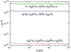
Figure 1. The cross sections for quenching of the metastable O2(b ) by O2(X
 , the energy transfer reaction O(1D) + O2(X
 , and detachment from O− by O2(b
 ).
).
Download figure:
Standard image High-resolution imageThe cross section for scattering of  molecules by
  molecules is assumed to be the same as for ground state molecules and is taken from Brunetti et al [26] and extrapolated to high and lower energy assuming a constant cross section. For the charge exchange
  + O2(b
 ) → O2(X
 +
+  , the cross section is assumed to be the same as for the ground state molecule and is taken from the literature [27–29], as discussed in our earlier work [14]. Similarly, the cross section for the charge exchange O+ + O2(b
 ) →
) →  + O is assumed to be the same as for the ground state and is taken from Lindsay and Stebbings [30]. All the reactions that are added here to the discharge model for oxygen are listed in table 1 along with the citation to the source for cross section or the rate coefficient used to estimate the cross section.
3. Secondary electron emission yield for oxygen bombarding metals
The emission of secondary electrons as a result of ions or neutrals bombarding a metallic surface plays an important role in discharge physics. Ion- and neutral-induced secondary electron emission has been studied both theoretically and experimentally for decades. In first approximation, the secondary electron emission yield is independent of the velocity of the bombarding particle for low energies, since the electron emission occurs due to transfer of the incoming ion or atom's potential energy to an electron in the target [36–38]. Considering that the ionization energies of O+ and  are 13.6 eV and 12.1 eV, respectively [39], i.e. they only differ by about 10%, we might expect that the potential secondary electron yield to be similar for O+ and
  . In accordance with this, Mahadevan et al [40] measured the secondary electron emission yield of O+ to be only 30% higher than of
  , for oxygen bombarding clean molybdenum and with a bombarding ion kinetic energy of around 50 eV. Kinetic emission, occurring when a bombarding particle transfers sufficient kinetic energy to an electron in the target, starts contributing to the total yield at a threshold energy of around a few hundred electron volts and dominates at higher energies. Both experimental data and theory predict a linear dependence of the secondary electron emission yield on the bombarding energy close to the threshold energy, and linear dependence on the bombarding velocity at higher energies [38, 41–43]. According to the theory of Parilis and Kishinevskii [41], the linearly dependent increase with increase in energy starts at a bombarding velocity of around
  m s−1, and the linearly dependent increase with velocity at around
  m s−1. At much higher energies, experimental data shows that the electron yield starts decreasing with increasing bombarding velocity. This occurs for a bombarding energy of around 100 keV for H+ [43]. Since the projectiles in our simulations have energies of at most around 500 eV, we do not expect this effect to have influence in our work and thus we do not include it in our fits. The energy threshold for kinetic energy emission is much larger than the bond energy of an oxygen molecule (5.17 eV at 298 K [44]), so in the kinetic emission regime we expect a bombarding oxygen molecule to behave as two independent oxygen atoms. A deviation from this is called a molecular effect. Experimentally, almost no molecular effect is measured [45, 46], although sometimes twice the yield of O+ is found to be 10%–30% higher than the yield of
  , at the same bombarding velocity [40, 47–51]. The reason for the molecular effect is not known at present [49, 52, 53], but Ferrón et al [54] suggest that if the oxygen ion beam contains a fraction f of the ion
  , then the atomic yields would increase by a factor 1 + 2f. The two different mechanisms are considered to be detachable, so the total electron emission yield is written as

where  and
and  are the contributions from potential and kinetic emission to the total yield, respectively.
The condition of the target significantly affects the ion-induced secondary electron emission yield. Clean metals, i.e. metals free of oxidation, gas adsorbtion, and other contamination, generally have a lower kinetic emission yield than contaminated metals [38, 42, 43, 55–59]. Heating in vacuum is usually not sufficient to obtain a clean surface, an evaporation in UHV or sputter cleaning with non-reactive ions is needed. The difference between early and more recent measurements of secondary electron emission yield is usually attributed to contamination on the metal surfaces of the earlier measurements due to inadequate cleaning [43]. Furthermore, experiments have failed to give reproducible results of the emission yield of oxidized metals. It has been hypothesized that this is due to changes in work function with different amounts of adsorbed and absorbed oxygen in the metal. Since electrons are more strongly bonded in adsorbates than in metals [59], there is a suppression of potential emission when oxygen is adsorbed on the surface. Agarwala and Fort [60] showed that the work function of oxygen-covered aluminum is highly dependent on the temperature and oxygen pressure of the oxygen gas the metal is exposed to when the oxygen layer is forming its surface, but in all cases the work function decreases compared to a clean aluminum surface. A stable layer will form, consisting of both surface oxygen and oxygen incorporated in the metal. Ferrón et al [54] showed that for Ar+ ions bombarding aluminum and molybdenum metals, the secondary electron emission yield is highly dependent on the target's oxygen exposure, and the dependence of the yield on exposure is qualitatively similar to the change in work function with oxygen exposure. They suggest that if oxygen is absorbed below the surface, the work function ϕ is lowered, but if oxygen is adsorbed on the metal, ϕ increases with increased amount of adsorbed gas. However, they also showed that changes in the work function cannot fully explain the change in magnitude of the secondary electron emission yield, and the yield is most likely also influenced by a change in the surface barrier caused by the adsorbed or absorbed oxygen in the metal, and by electrons emitted from the oxide layer due to the surface dipole field [54, 59].
3.1. Fits of secondary electron emission yield as a function of energy for oxidized metals
The data we collected from the literature on the ion-induced secondary electron yield of oxygen species bombarding contaminated metal surfaces is shown in figures 2 and 3 for  -ions and O+ -ions, respectively. In order to make a fit of the secondary electron emission yield to implement into oopd1, we seek data for a metal that would best represent the metal in a capacitively coupled rf discharge. We furthermore look for data for oxidized metals as targets, since we are simulating a steady state. The measurements by Chen [61] for oxygen bombarding aluminum were taken for a piece of aluminum foil that was not treated by sputtering or heating, and Auger electron spectroscopy (AES) showed that the surface was heavily oxidized. Furthermore, aluminum is a material commonly used for electrodes in capacitively coupled oxygen discharges. This data is the only data we found with a surface that could represent discharge conditions, and hence it is the only data we will use for our fit. The fit, shown in figures 2 and 3, lies close to the data of Wittmaack [49], and Yamauchi and Shimizu [62], who found by AES that the aluminum surface used as target was oxidized even though it had been bombarded with 2 keV argon ions prior to measurements. However, our fit for the yield is three orders of magnitude larger than the data collected by Parker [63], in the potential energy regime. He exposed platinum and tantalum targets to oxygen gas before measuring the oxygen ion induced secondary electron emission, without distinguishing whether
  or O+ had been the bombarding species. The surface was not characterized by AES, but since platinum does not oxidize in air at any temperature, and tantalum is not reactive at temperatures below 150 °C, we expect the oxygen to be absorbed on the surface [64]. As previously discussed, this should lower the potential emission significantly compared to if the gas were adsorbed in the metal. Similarily, our fit for the yield lies significantly higher than the yield of oxygen bombarding copper, measured by Chen [61]. This can possibly be explained by the fact that copper reacts slowly with oxygen at standard conditions, and AES showed that the copper surface used had similar transition peaks as a clean surface, although impurities of Cr, S and Cl were detected. The secondary electron emission yield of oxygen bombarding copper was not taken at normal incidence, and the data displayed on the graph is found with the formula
  [65–68], where
  is the yield at an incident angle of θ.
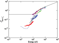
Figure 2. Electron yield of  ions bombarding untreated metal surfaces, along with a fit to the data as explained in the text. (×) Al [62] (— - —) Ta [63]; (•) Pt [63]; (
 ) Al [61]; (
 ) Cu [69]; (
 ) Mo [40]; (◦) Al [49]; (
 ) Si [49]; (
 ) n-Si [50]; (•) Cu (60° incidence) [61]; (−) fit to the data as explained in text.
Download figure:
Standard image High-resolution image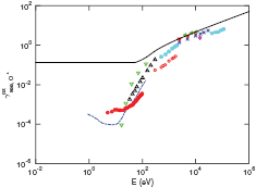
Figure 3. Electron yield of O+ ions bombarding untreated metal surfaces, along with a fit to the data as explained in the text. ( ) n-Si [50]; (— - —) Ta [63]; (•) Pt [63]; (
 ) Cu [70]; (
 ) SS [71]; (
 ) Al [49]; (
 ) untreated Mo [40]; (◦) monolayer-covered Mo [40]; (
 ) Cu (measured in lab) [69]; (
 ) Cu (measured in satellite) [69]; (×) Inconel 625 [72]; (−) fit to the data as explained in text.
Download figure:
Standard image High-resolution imageIn our fit for the yield of  bombarding oxidized aluminum, we use a constant value of
  in the potential energy regime, and a value of
  that varies linearly with bombarding ion velocity for high bombarding energies. The constant
  is taken to be the mean value of the data points of Chen [61] at an energy lower than 120 eV. The data points between 120 eV and 500 eV were fitted by a 3rd degree polynomial. The threshold energy, when kinetic energy starts to make a contribution and the yield is no longer constant, was taken to be the intersection of the polynomial with the constant value chosen for
  . A linear fit in bombarding velocity was found using data points for bombarding velocities higher than
  . This linear fit was forced to pass through the point of the 3rd degree polynomial at 500 eV energy and is used for bombarding energy values higher than 500 eV.
The fit for  as bombarding species on oxidized metal target is as follows:

where E is the energy of the incoming ion in the lab frame in eV,  is the mass of an oxygen molecule, and e is the elementary charge. When developing a fit for O+ , we do not assume any molecular effects to take place, so the kinetic emission of O+ is assumed to be half the kinetic emission of
  at the same bombarding velocity, i.e.
where E is the energy of the incoming O+ ion, and  and
and  are the secondary electron kinetic emission yields for O+ and
  respectively. We assume that the potential emission yield is the same for O+ and
  , i.e.
  =
=  . The fits for
  and O+ are plotted in figures 2 and 3, respectively. Even though no data for O+ as bombarding ions was used to make the fit, it can be seen in figure 3 that the fit lies very close to the aluminum data points.
Amme [73] measured the secondary electron yield for O2 neutrals with lab energy in the range 100–1000 eV. The target material itself is not specified, but it is untreated, and H2O is assumed to be the principal absorbed species. We found a 3rd degree polynomial fit to the measured values on a log–log scale and used for our fit for the secondary electron emission yield of neutral O2 bombarding the electrodes in the plasma discharge. Since species in our simulation do not have energy higher than around 500 eV, and we have data up to 1000 eV, we do not use a linear model for higher energies. The formula for the fit is:
where E is the energy of the incoming molecule in the lab frame in eV. Since only kinetic emission occurs for neutral atoms and molecules in the ground state, the secondary electron emission yield for neutral O  is taken to be half the value of the secondary electron emission yield for neutral O2
  computed at twice the bombarding energy of the neutral O, i.e.

The data points from Amme [73] and the fits can be seen in figure 4.
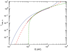
Figure 4. Electron yield of O2 molecules bombarding an untreated metal surface, and a fit to the data. (−) [73]; (−−) fit to the data for neutral O2 as explained in text; (⋯) fit for neutral O as explained in text; (– - –) kinetic emission of  .
.
Download figure:
Standard image High-resolution imagePotential emission does not occur for neutrals, and kinetic emission depends, in first approximation, only on the bombarding velocity of the incoming ion or neutral so the neutral-induced secondary electron emission yield might be taken to be only the kinetic emission yield of the corresponding ion. The kinetic emission of  is plotted in figure 4. It agrees well with our fit in the energy range 100–1000 eV, but since the threshold energy for kinetic emission was taken to be around 100 eV, the kinetic emission of
  is taken to be zero below that threshold in our fit. Medved et al [74] did not find the kinetic emission yield to be the same for neutral Ar (
 ) and Ar ions (
 ) bombarding clean molybdenum. In particular, they measured
  = 1.5, where E is the projectile's energy. Furthermore, Lakits et al [75] did not find
  to be constant for H, He, Ne and Ar bombarding clean gold. This was explained by a semiempirical theory, assuming that the projectile electrons screen the cores differently in neutrals and ions when the projectile penetrates the solid. Thus, we implement the fit to the data by Amme [73] in oopd1, instead of assuming that the kinetic emission of neutral O2 is the same as for the ion
  .
.
3.2. Fits of secondary electron emission yield as a function of energy for clean metals
Experimental data from the literature for  bombarding clean metal surfaces are shown in figure 5. We made a 4th degree polynomial fit to all data available, except the 8 lowest energy data points of Mahadevan et al [40] and the data of Cawthron et al [45]. The data points of Mahadevan et al [40] are ignored since the surface might not have been atomically clean [76] and the potential emission they measured is considerably larger than the measurements of Vance [77] and Propst and Lüscher [78]. However, the data of Cawthron et al [45] is ignored since it was not taken at normal incidence. The data displayed on the graph is found with the formula
  . However, the yield can deviate considerably from this formula [50, 79], which is why the data is not included in the fit. The 4th degree polynomial was made to fit log–log data and we used the method of least squares. The potential energy emission was taken to be the constant
  , which is the value of the polynomial at the data point with the lowest energy measurement of around 26 eV, made by Vance [77]. This value is used for the yield of particles with energy lower than 26 eV. We expect the kinetic emission threshold to be much higher than 26 eV, but since measurements exist in the low-energy regime, they were used to make a polynomial fit, instead of assuming constant potential emission. The highest three values of
  available, measured by Large [46], were used to make a linear fit in velocity for high bombarding energies. This data was used for the fit for bombarding energies higher than 184.32 keV, which is the intercept of the line for high bombarding energies, and the 4th degree polynomial for intermediate energies.

Figure 5. Electron yield of  ions bombarding clean surfaces, along with a fit to the data as explained in the text. (+) Al [81]; (
 ) W [47]; (⋯) Pt (45° incidence) [45]; (−−) C (45° incidence) [45]; (— - —) Ta (45° incidence) [45]; (
 ) C [51]; (
 ) Mo [48]. (
 ) W [46]; (
 ) Mo [40]; (
 ) W [78]; (
 ) Mo [77]; (
 ) n-Si [50].
Download figure:
Standard image High-resolution imageExperimental data from the literature for O+ bombarding clean metal surfaces is shown in figure 6. We made a 4th degree polynomial fit to all data available (with the exceptions discussed below) that had a bombarding energy higher than 1000 eV, using the method of least squares. The polynomial was made to fit log–log data. The potential electron emission was taken to be a constant  , which is deduced both from the graph and from the potential emission found for
  below, using that the potential emission should be similar for O+ and
  . The reason why the value of
  is taken to lie farther away from the data of Mahadevan et al [40] than other data available, is that it was argued by Vance [76] that their method of cleaning the Mo target was not sufficient to clean the metal of all carbon contamination. The constant potential emission was used for the fit for bombarding energies lower than 370.35 eV, which is the intercept of the constant potential emission, and the 4th degree polynomial for intermediate energies. The highest three values of
  available, from Cook and Burtt [47] were used to make a linear fit in velocity for high bombarding energies. This data was used for the fit for bombarding energies higher than 16.837 keV, which is the intercept of the line for high bombarding energies, and the 4th degree polynomial for intermediate energies. The data of Cawthron et al [45, 80] was not used for the fit, as the ions were not bombarding the metals at normal incidence as for the rest of the data. The data displayed on the graph is found with the formula
  .
.
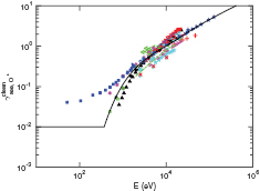
Figure 6. Electron yield of O+ ions bombarding clean surfaces, along with a fit to the data as explained in the text. (+) Al [81]; ( ) Pt (45° incidence) [80]; (
 ) Ta (45° incidence) [80]; (
 ) C (45° incidence) [80]; (
 ) Ni (45° incidence) [80]; (−−) C (45° incidence) [45]; (⋯) Pt (45° incidence) [45]; (— - —) Ta (45° incidence) [45]; (✶) C (the black and magneta colors correspond to bombarding of surfaces with high and low thermal conductivity, respectively) [82]; (
 ) W [47]; (•) C [51]; (
 ) Mo [48]; (
 ) Al [83]; (⋆) W [46]; (
 ) HOPG [84] (
 ) Au [85]; (
 ) Mo [40]; (
 ) Mo [86]; (
 ) n-Si [50]; (◦) Mg [87]; (
 ) Al [87]; (×) Si [87].
Download figure:
Standard image High-resolution imageThe fit for  as bombarding species on clean target is:
and the fit for O+ as bombarding species on clean target is:
4. The simulation
We assume a capacitively coupled discharge where one electrode is grounded and the other is driven by an rf voltage,

where t is the time, f is the frequency and V0 is the peak voltage. As in our earlier work [4, 14], we assume the discharge to be operated at a single frequency of f = 13.56 MHz, with electrode separation of 4.5 cm, and electrode diameter of 14.36 cm. The electrode diameter is needed to get the discharge volume for global model calculations and for calculating the absorbed power. A large, 1 F capacitor is assumed to be in series with the voltage source. Nine species are treated kinetically; electrons, the negative ions O−, the positive ions O+ and  , the metastable oxygen atom O(1D), the metastable oxygen molecules
  and O2(b
 , and the neutral species O(3P) and
  . The full oxygen reaction set was used in the simulation, as listed in our earlier works [4, 14] and in table 1. The charged particles are tracked at all energies, but since the neutral species density in the plasma is much higher than the density of the charged particles, the neutrals are only treated kinetically if their energy reaches a preset threshold value, listed in table 2. Neutrals with energy less than the threshold energy are treated as background species with fixed density and temperature, maintained uniformly in space and assumed to have a Maxwellian velocity distribution at the gas temperature (here
  = 26 mV). A volume averaged (global) model is used to determine the partial pressure for the neutral species at 50 mTorr [88], and these values are used for all pressures studied. The partial pressures used here are 0.52% for O(3P), 0.028% for O(1D) and 4.4% for O2(
 ). When the species O2(b
 is included in the discharge model, we assume the partial pressures 90.65%
  and 4.4% O2(b
 , but 95.05%
  when it is excluded, unless otherwise stated. Other combinations of singlet metastable partial pressures are also explored. The wall quenching and recombination coefficient for the neutrals are listed in table 2. For this study we assume that as an energetic oxygen molecule in the ground state O2(X
 hits the electrode it returns as a thermal O2(X
 with 100% probability. We use recombination coefficient of 0.5 for O(3P) and O(1D) at the electrodes as measured by Booth and Sadeghi [89] for pure oxygen discharge in a stainless steel reactor. This may be a bit high value and thus underestimate the oxygen atom density. We assume quenching probability of 0.5 for O(1D) hitting the electrode. For the metastable molecule O2(
 ) we use a quenching probability of 0.007 estimated by Sharpless and Slanger [90] for iron. Their estimate for aluminum is <10−3. Greb et al [91] argue that increasing the quenching coefficient leads to decreased O2(a
 ) density and thus decreased detachment by the O2(a
 ) state and thus higher negative ion density. For iron Ryskin and Shub [92] report a value of 0.0044 and a value of
  for aluminum. Using the values for aluminum electrodes would therefore lead to higher singlet metastable densities and lower electronegativity. We have seen in global model studies that wall quenching can be the main loss mechanism for the singlet metastable state O2(b
 ) [8]. In these studies we assumed that the quenching coefficient to be 0.1, which is the same value as we assume in this current study. This assumption is based on the suggestion that the quenching coefficient for the b
 state is about two orders of magnitude larger than for the a
 state [93]. The particle weight is the ratio of the number of physical particles to computational particles, i.e. the number of real particles each superparticle represents. In oopd1, different weights of particle species can be implemented. The particle weights used here are displayed in table 2 as well. The simulation grid is uniform and consists of 1000 cells, and the electron time step is
  s. The grid spacing
  and time step are chosen such that the electron plasma frequency is resolved adequately, and such that the electron Debye length of low-energy electrons satisfies
  , where
  is the electron plasma frequency. A sub-cycling factor of 16 was used for heavy particles and their initial density profiles are chosen to be parabolic [94]. The simulation was run for
  time steps or 2750 rf cycles.
Table 2. The parameters of the simulation, the particle weight, the threshold above which dynamics of the neutral particles are followed and the wall recombination and quenching coefficients used.
| Species | Particle weight | Threshold (meV) | Wall quenching or recombination coefficient |
|---|---|---|---|
 |
 |
500 | 1.0 |
O2( ) ) |
 |
100 | 0.007 [90] |
O2(b |
 |
100 | 0.1 |
| O(3P) |  |
500 | 0.5 |
| O(1D) |  |
50 | 1.0 (0.5 rec., 0.5 quench.) |
 |
107 | — | — |
| O+ | 106 | — | — |
| O− |  |
— | — |
5. Results and discussion
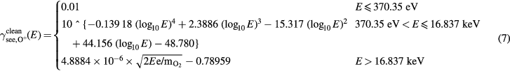
Figure 7 shows the density profiles of the charged particles and high energy neutral particles at 50 mTorr and V0 = 222 V when the simulation includes the energy-dependent secondary electron emission yield given in section 3 for oxidized metal surfaces, and for simulations excluding and including the metastable O2(b . As seen when comparing figures 7(a) and (c), the presence of O2(b
 changes the composition of the discharge significantly. When O2(b
 is excluded from the simulation as seen in figure 7(a), the density of the ions
  and O− is dominating in the plasma bulk (the electronegative core), and the electron density is smaller. When O2(b
 ) is included in the simulation as seen in figure 7(c), the density of
  -ions and electrons dominate in the plasma bulk and the O− density is smaller. In both cases the O+ density is negligible compared to the other charged particles. The density profiles for high energy neutrals, shown in figures 7(b) and (d) are considerably different from the ones found in Gudmundsson and Lieberman [4], in particular the atomic oxygen profile. This is due to a previous bug in our code, which led to too many neutrals being created in the discharge. The correct density profile for neutral oxygen atoms is now cosine like, for both O(3P) and O(1D). This is typical for neutral species where wall losses dominate and in accordance with the measurements of Katsch et al [95]. They measured a cosine like profile for atomic oxygen in a 13.56 MHz discharge, at a peak voltage of 200 V and 490 mTorr pressure. The metastables O2(a
 ) and O2(b
 , however, are more abundant near the electrodes than in the bulk. Both of these metastable molecular states are relatively stable towards wall quenching, while the neutral oxygen atoms are not. The density of the metastables O2(a
 ) and O2(b
 are almost identical, since the electron impact excitation reactions e + O2(X
 e + O2(a
 ) and e + O2(X
 e + O2(b
 are the dominant production mechanisms for high energy molecular oxygen metastables, and these two reactions have similar cross sections but the cross section for the creation of O2(a
 ) is slightly larger and has a lower threshold. Thus the metastable O2(a
 ) is slightly more abundant in the bulk region.
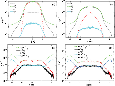
Figure 7. The density profile for charged particles (a) excluding the species O2(b and (c) including the species O2(b
 in the simulation, and the density profiles of high energy neutral particles (b) excluding the species O2(b
 and (d) including the species O2(b
 in the simulation, in a parallel plate capacitively coupled discharge at 50 mTorr with a gap separation of 4.5 cm driven by a 222 V voltage source at 13.56 MHz.
Download figure:
Standard image High-resolution imageFigure 8 shows the density profiles for  -ions, O−-ions and electrons at 50 mTorr. We explore the difference between the case when only the singlet metastable O2(a
 ) is included in the simulation, and the cases when both of the singlet metastables O2(a
 ) and O2(b
 ) are included at various partial pressures. Furthermore, we examine the effects of including the energy-dependent secondary electron emission yield. The peak
  -density is highest when only the O2(a
 ) state is included in the simulation as seen in figure 8(a). We see in figure 8(a) that the peak
  -ion density drops with increasing partial pressure of the singlet metastable O2(b
 ). However, adding the energy-dependent secondary electron emission increases the
  peak density. We also see that the
  -ion density profile widens with the addition of energy-dependent secondary electron emission. Similar behavior is observed for O−-ions as seen in figure 8(b), that is, the peak O−density decreases with increased partial pressure of O2(b
 ) in the discharge. The addition of the singlet metastable O2(b
 ) leads to an increase in the electron density as seen in figure 8(c) and the electron density profile is almost independent of the partial pressures of O2(a
 ) and O2(b
 ) when both are included. This is due to very efficient detachment process by the singlet metastable molecules. When the energy-dependent secondary electron emission is added to the discharge model the electron density increases even more, since electrons created at the electrodes are accelerated across the sheath and increase the ionization in the plasma bulk.
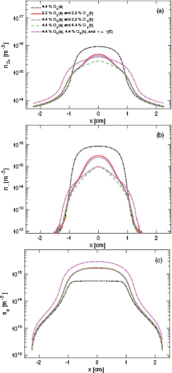
Figure 8. The (a)  -ion density profile, (b) O−-ion density profile, and (c) electron density profile for a parallel plate capacitively coupled oxygen discharge at 50 mTorr with a gap separation of 4.5 cm driven by a 222 V voltage source at 13.56 MHz.
Download figure:
Standard image High-resolution imageFigure 9(a) shows the profile of the power absorption by the electrons at 50 mTorr, given by  , where
  and
and  are the spatially and temporally varying electron current density and electric field, respectively. When the singlet metastable O2(b
 ) is added to the discharge model, the electron heating is entirely in the sheath region, so no ohmic heating occurs in the plasma bulk. Varying the partial pressures of O2(
 ) and O2(b
 ) has little effect on the heating profile. When only the singlet metastable molecule O2(
 ) is included in the simulation the peak heating rate in the sheath region is slightly lower than when O2(b
 ) is included, and there is some ohmic heating in the plasma bulk. When the energy-dependent secondary electron emission is added to the discharge model, the electron heating rate increases and occurs closer to the electrodes, so the sheaths become narrower. A concave or bi-Maxwellian shape of the EEPF, as seen in figure 9(b), has been associated with predominant sheath heating [6, 97]. We have discussed elsewhere how the presence of the metastable molecule O2(
 ) leads to this concave shape of the EEPF [4]. Furthermore, when adding the energy-dependent secondary electron emission yield, the EEPF becomes even more concave. The EEPF is related to the EEDF through
  where
where  is the EEPF,
  is the EEDF and
  is the electron energy. The EEPF is roughly independent of the partial pressure of O2(
 ) and O2(b
 ) when both are included in the model. When including an energy-dependent secondary electron emission yield, more electrons are created at the electrodes, which are accelerated to the bulk due to the potential difference between the electrode and bulk plasma. Thus more high energy electrons are created in the discharge and the EEPF develops a high energy tail.

Figure 9. The (a) electron heating rate profile and the (b) electron energy probability function (EEPF) in the center of for a parallel plate capacitively coupled oxygen discharge at 50 mTorr with a gap separation of 4.5 cm driven by a 222 V voltage source at 13.56 MHz.
Download figure:
Standard image High-resolution imageFigure 10 shows the electron heating rate profile and the EEPF in the pressure range 10–500 mTorr, for V0 = 400 V, with both O2(b ) and the energy-dependent secondary electron emission yield included in the simulation. As discussed by Gudmundsson and Ventéjou [5], ohmic heating in the bulk plasma dominates at low pressures (10 mTorr), but at higher pressures (50–500 mTorr), the electron heating occurs almost solely in the sheath region. When both the singlet metastable states are included in the simulation model, the ohmic heating in the plasma bulk is essentially zero in the pressure range 50–500 mTorr as seen in figure 10(a).
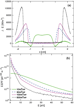
Figure 10. The (a) electron heating rate profile and the (b) electron energy probability function (EEPF) in the center of for a parallel plate capacitively coupled oxygen discharge with a gap separation of 4.5 cm driven by a 400 V voltage source at 13.56 MHz.
Download figure:
Standard image High-resolution imageFigure 11 shows the density at the center of the discharge for  -ions, O−-ions and electrons as a function of pressure, in the pressure range 5–100 mTorr. We show three cases, including only the metastable O2(a
 ) (◦), including only both the singlet metastable metastable states O2(a
 ) and O2(b
 ) (+), and including both the singlet metastable states and an energy dependent secondary electron emission yield (x), in the simulation. When the metastable O2(b
 ) is excluded from the simulation, the density of
  -ions and O−-ions at the discharge center is approximately constant with increasing pressure, but when it is included the O−-ion density is monotonically decreasing with increasing pressure and the
  -ion density decreases with increasing pressure to a minimum at 40 mTorr and then increases again with further increase in pressure. This is in accordance with the measurements of Stoffels et al [98], who found the O−-ion density in a capacitively coupled discharge with 30 sccm gas flow and 10 W input power to decrease from around
  m−3 to
  m−3 in the pressure range 30–200 mTorr. However, they measured a decreasing density with decreasing pressure below 30 mTorr, which we did not see in our simulations. Adding energy-dependent secondary electron emission yield increases the
  -ion density and the electron density slightly. In figure 12, the electron density from our simulations is compared to the measurements of Kechkar [96]. In his experiment, the discharge was slightly asymmetric, as the diameter of the driven electrode was 205 mm, but 295 mm for the grounded electrode. We simulated this case with both electrodes of area 330 cm2, which corresponds to the smaller diameter. The voltage values used in our simulations correspond to Kechkar's [96] input power of 200 W. When the metastable O2(b
 ) and energy-dependent secondary electron emission yield are included in the discharge model, the results agree very well with the measurements of electron density by Kechkar [96], in the entire pressure range 100–600 mTorr.

Figure 11. The (a)  -ion density, (b) O−-ion density, and (c) electron density at the center as a function of pressure for a parallel plate capacitively coupled oxygen discharge with a gap separation of 4.5 cm driven by a 222 V voltage source at 13.56 MHz. (+):
  , 4.4% O2(a
 ) and 4.4% O2(b
 ); (◦):
  , 4.4% O2(a
 ); (x):
  , 4.4% O2(a
 ) and 4.4% O2(b
 ).
).
Download figure:
Standard image High-resolution image
Figure 12. The electron density at the center as a function of pressure for a parallel plate capacitively coupled oxygen discharge with a gap separation of 4.5 cm driven by a 200 W voltage source at 13.56 MHz. (+):  , 4.4% O2(a
 ) and 4.4% O2(b
 ); (◦):
  , 4.4% O2(a
 ); (x):
  , 4.4% O2(a
 ) and 4.4% O2(b
 ); (
); ( ) Measurements from Kechkar [96].
Download figure:
Standard image High-resolution imageFigure 13 shows the comparison of the calculated and measured effective electron temperature in the discharge center ( where
where  is the average electron energy) as a function of pressure. The center effective electron temperature decreases as the pressure is increased, from around 7 V at 10 mTorr to less than 1 V at 100 mTorr, in the case where both the metastables O2(
 ) and O2(b
 ) are included in the discharge model. The addition of the singlet metastable O2(b
 ) has a significant influence on the effective electron temperature. At 50 mTorr the center effective electron temperature drops from 1.4 V when only the singlet metastable O2(
 ) is included in the simulation, to about 0.7 V when the singlet metastable O2(b
 ) is added along with the relevant reactions. The effective electron temperature drops further, to around 0.5 V, when the energy-dependent secondary electron emission yield is added to the simulation model. The drop in the effective electron temperature in the discharge center indicates that the heating of the electrons is effective in the sheath region, but the ohmic heating in the discharge center is ineffective. Earlier, we showed that when the metastables O2(
 ) and O2(b
 ) are excluded from the simulation, the effective electron temperature is parabolic in shape, that is, the temperature does not drop in the discharge center [4]. Thus it is essential to include the singlet metastable states in the simulation in order to get the effective electron temperature and the electron heating mechanism correct. The results of our simulations are compared to the measurements of Kechkar [96] in figure 13. In the intermediate pressure range (50–200 mTorr), our results agree well with the measured values. As shown in Gudmundsson and Lieberman [4], adding the metastable O2(
 ) to the discharge model at 222 V and 50 mTorr lowers the effective electron temperature from around 3.3 eV to around 1.7 eV, and here we show that by adding the metastable O2(b
 ) further lowers the electron temperature to values below 1 eV. This is in accordance with the measurements of Kechkar [96] which find
  eV in the pressure range 50–200 mTorr in a pure oxygen discharge. Furthermore, the measurements of Pulpytel et al [99] measured the effective electron temperature in an Ar/O2 (
 ) mixture at 110 mTorr and voltages above 300 V to be around 1 eV. However, we note that the measured effective electron temperature at 400 and 600 mTorr is much higher than the simulations predict.
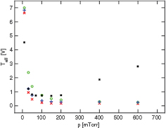
Figure 13. The effective electron temperature at the center of the discharge as a function of pressure for a parallel plate capacitively coupled discharge with a a gap separation of 4.5 cm driven by a 200 W voltage source at 13.56 MHz. (+):  , 4.4% O2(a
 ) and 4.4% O2(b
 ); (◦):
  , 4.4% O2(a
 ); (x):
  , 4.4% O2(a
 ) and 4.4% O2(b
 ); (
); ( ) Measurements from Kechkar [96].
Download figure:
Standard image High-resolution imageFigure 14(a) shows the variation of the effective electron temperature at the center of the discharge at 50 mTorr with the discharge peak voltage V0. When the metastable O2(b ) is included in the discharge model, the effective electron temperature at low operating voltages of around 100 V are significantly smaller than at 500 V, contradictory to the case when O2(b
 ) is excluded. At all voltages explored, the energy-dependent secondary electron emission decreases the effective electron temperature somewhat. Furthermore, figure 14(b) shows the variation of the center electronegativity
  /
/ at 50 mTorr with voltage, where n−0 is the center negative ion density and
  is the center electron density. The electronegativity decreases with increased voltage for voltages above 300 V. When the metastable O2(b
 is included in the discharge model, the electronegativity at 100 V is lower than at 500 V, but when it is excluded, the electronegativity seems to be almost monotonically decreasing with increasing voltage, except for a small peak around 200 V. Gudmundsson and Ventéjou [5] showed that in a capacitively coupled oxygen discharge at 50 mTorr, 13.56 MHz and 222 V, the electronegativity drops from about 63 when no metastables are included to around 15 when the metastable O2(a
 is included, due to the effective detachment by the O2(a
 molecule. Including the metastable O2(b
 ) in the discharge model further lowers the electronegativity to around 0.52, and including an energy-dependent secondary electron emission yield lowers it even further to 0.33. As can be seen in figure 8, this decrease by almost two orders of magnitude is due to both an order of magnitude's decrease in the O−-ion density and an order of magnitude's increase in electron density, when the metastable O2(b
 ) and the energy-dependent secondary electron emission yield are included in the discharge model, compared to when only O2(a
 is included.

Figure 14. The (a) effective electron temperature and (b) electronegativity at the center of the discharge for a parallel plate capacitively coupled discharge at 50 mTorr with a a gap separation of 4.5 cm at 13.56 MHz. (+):  , 4.4% O2(a
 ) and 4.4% O2(b
 ); (◦):
  , 4.4% O2(a
 ); (x):
  , 4.4% O2(a
 ) and 4.4% O2(b
 ).
).
Download figure:
Standard image High-resolution imageFigure 15 shows the variation of the center  -ion density, O−-ion density and electron density as a function of the peak voltage applied to the discharge. The center
  -ion density and O−-ion density decrease when the metastable O2(b
 ) is added to the discharge model, and the electron density increases. Including the energy-dependent secondary electron emission yield increases the
  -ion and electron density, and the increase gets larger with higher applied voltage. Adding energy-dependent secondary electron emission has little effect on the negative ion density.
Figure 15. The electron density as a function of peak voltage for a parallel plate capacitively coupled oxygen discharge at 50 mTorr with a gap separation of 4.5 cm at 13.56 MHz. (+):  , 4.4% O2(a
 ) and 4.4% O2(b
 ); (◦):
  , 4.4% O2(a
 ); (x):
  , 4.4% O2(a
 ) and 4.4% O2(b
 ).
).
Download figure:
Standard image High-resolution image
6. Conclusion
The one-dimensional object-oriented particle-in-cell Monte Carlo collision code oopd1 was applied to explore the influence of the singlet metastable molecules O2( ) and O2(b
 ) on the oxygen discharge. We find that detachment by the singlet metastable molecules O2(a
 ) and O2(b
 ) has a significant influence on the discharge properties such as electronegativity, effective electron temperature and electron heating processes in a capacitively coupled oxygen discharge. Earlier we had demonstrated that the heating mechanism changes significantly when the metastable molecule O2(a
 ) is included in the reaction set [4], mainly due to the detachment by the singlet metastable molecule. Thus we have demonstrated that in order for the electron kinetics of the discharge to be correct when simulating an oxygen discharge, the singlet metastable O2(a
 ) has to be included in the discharge model. This is particularly important for discharge pressure above 30 mTorr. Furthermore, in order to fine tune the electron heating processes the singlet metastable O2(b
 ) has to be included as well, along with energy dependent secondary electron emission yield. The energy dependent secondary electron emission yield has an influence on the width of the electronegative core (the sheath width) and in particular the electron density profile.
We developed a fit for an energy-dependent secondary electron emission yield for O+ -ions,  -ions, O-atoms and O2 molecules bombarding both clean and oxidized metal electrodes and incorporated these into the oopd1 code. An energy-dependent secondary electron emission yield changes the discharge properties such as the density profiles of ions, electron heating rate, EEPF and effective electron temperature. The sheath width decreases and the density of electrons and the density of
  -ions in the discharge center increases when secondary electron emission is included. In our simulations, only the secondary electron emission yield of the ion
  contributes significantly to the discharge properties, and the secondary electron emission due to the ion O+ and the neutrals is negligible. The simulation results for both electron density and effective electron temperature agree very well with experimental findings, in particular the effective temperature is found to be
  eV in the pressure range 50–200 mTorr.
Acknowledgments
We are grateful to Dr Samir Kechkar for providing us unpublished experimental data.
This work was partially supported by the Icelandic Research Fund Grant Nos. 130029-053 and 163086-051 and the Swedish Government Agency for Innovation Systems (VINNOVA) Contract No. 2014-04876.