


Abstract
Digital holography is a valuable tool for three-dimensional information extraction. Among existing configurations, the originally proposed set-up (i.e. Gabor, or in-line holography), is reasonably immune to variations in the experimental environment making it a method of choice for studies of fluid dynamics. Nevertheless, standard hologram reconstruction techniques, based on numerical light back-propagation are prone to artifacts such as twin images or aliases that limit both the quality and quantity of information extracted from the acquired holograms. To get round this issue, the hologram reconstruction as a parametric inverse problem has been shown to accurately estimate 3D positions and the size of seeding particles directly from the hologram. To push the bounds of accuracy on size estimation still further, we propose to fully exploit the information redundancy of a hologram video sequence using joint estimation reconstruction. Applying this approach in a bench-top experiment, we show that it led to a relative precision of 0.13% (for a 60 μm diameter droplet) for droplet size estimation, and a tracking precision of  .
.
Export citation and abstract BibTeX RIS
1. Introduction
Optical diagnostics are reliable tools for fluid dynamics and studies in reactive environments. Their non-invasive nature makes it possible to extract quantitative information from the medium under investigation without disturbance. Among the available techniques, digital in-line holography enables reconstruction of a three dimensional volume from a single interference recording called a hologram. Moreover, unlike off-axis configurations, digital in-line holography is experimentally simple to implement and is almost immune to variations in the experimental environment (e.g. temperature evolution, vibrations), making it a method of choice for medium characterization in severe experimental conditions [1–5]. The recorded information is usually reconstructed by calculating light back-propagation from the sensor plane to a targeted plane in the volume under study [6, 7], leading to the extraction of three-dimensional information such as the velocity field, and the trajectories [8–11]. However, hologram reconstruction based on light back-propagation is prone to sampling artifacts and twin image disturbances [12–15], which limit the signal to noise ratio of the reconstructed holograms, as well as the accuracy of the estimated parameters of the object (3D positions x, y, z, and radius r for particle holography).
In contrast to these light back-propagation reconstruction methods, in certain cases, signal processing tools and their extensions to image processing may enable optimal processing [16]. Instead of transforming the hologram through numerical light back-propagation, the aim here is to find the imaging model parameters that best represent the recorded hologram [17, 18]. These 'inverse problems' (IP) approaches, which are sometimes referred to as compressive sensing methods [19–21], makes it possible to increase the accuracy of the reconstruction [22, 23] and to recover signal beyond the physical limits of the imaging sensor [24]. Among IP algorithms, the reconstruction of parametric objects is performed using greedy algorithms, objects are iteratively optimally detected and removed from the original hologram for SNR improvement. Exploiting information redundancy along a video sequence makes it possible to further improve the accuracy of the imaging model parameters, thereby performing joint parameter estimation [25, 26] or super resolution [27]. However, the accuracy of the reconstruction is achieved at the cost of computation time. Time processing issues can be solved by considering either software [28, 29] or hardware strategies [30, 31]. However, in this article, we focus on the algorithm that improves accuracy and leave aside problems of computation time.
To test the algorithm in bench-top experiments, we propose to use IP reconstruction algorithm to reconstruct and track droplets delivered, on demand, by a piezo-electric (PZT-) injector, using digital in-line holography. The PZT injector used in this experiment generates mono-dispersed water droplets. We consequently exploited the constancy of the radius during the course of the video hologram sequence to improve the accuracy of its measurement. Moreover, the assumption of free-falling objects gives a trajectory model that allowed us to estimate the accuracy of 3D positioning. We demonstrate that the proposed method is able to perform 3D droplet localization and tracking with a precision of  μm3 (or
  ), and with a precision of
  nm (or 0.13%) in the radius estimation (for a 30 μm water droplet).
2. Data acquisition and pre-processing
2.1. Experimental setup
Figure 1 shows the in-line holographic setup used for 3D tracking of free-falling droplets. This configuration is similar to that of [32]. The light emitted from a Nd-YVO4 solid state laser ( nm Millennia IIs Spectra Physics) is low pass filtered and expanded using a f = 100 mm focal-length lens associated with a 50 μm a diameter pinhole. The illumination beam is a spherical diverging wavefront impinging the water droplet jet under investigation. The jet consists of free-falling mono-dispersed water droplets generated by a piezo-electric injector (MJT-AT-01 MicroFab Technologies jetting device, 60 μm orifice diameter) located at 992 mm from the diaphragm and 472 mm from the imaging sensor. Interference between the field diffracted by the droplets and the reference beam (the part of the illumination beam that does not interact with the droplets) are recorded on a
  pixel CMOS sensor (Phantom V611) with a pixel pitch of 20 μm and operating at 6200 frames per second. It should be noted that no collection optics is used for the holographic recording. The pixel fill factor, representing the ratio of the active surface of the pixel to the physical surface of the pixel, can be accounted for in our imaging model according to [33] and is
  . The axial position of the water droplet is estimated roughly (based on the distance from the injector to the sensor) to be in the
  m to
m to  m range. To measure image magnification, the injection plane is considered as a reference plane. Magnification in the ith plane Gi was calibrated using a reticle and expressed as
  (see [35] for details about the calibration procedure). Here,
  is the algebraic distance between the injection and the ith planes (counted as positive in the light propagation direction). The z range
 ![$\left[{{z}_{\text{min}}};{{z}_{\text{max}}}\right]$](https://content.cld.iop.org/journals/0957-0233/27/4/045001/revision1/mstaa14c4ieqn012.gif) verifies
verifies  , with r the droplet radius. Under this assumption, the droplets can be viewed as opaque spherical objects and the Huygens–Fresnel integral, which gives the intensity recorded on the imaging sensor, has an analytical solution [36]. The intensity
  recorded for a spherical opaque particle at a distance of z from the imaging sensor is thus given by
where ϑ is the aperture function of the spherical droplet defined as
and  are the coordinates in the aperture (droplet) plane. The Fourier transform of ϑ can be analytically derived and is given by
where J1 is the Bessel function of the first kind. It should be noted that the squared term in equation (1) is negligible in our experimental conditions as  . In the case of a diluted sample, optical interaction between particles can be disregarded. Therefore, multiple particles can be considered with an additive intensity model given by
where  is the number of particles to be considered and i is the particle index. It should be noted that intrinsic in-line holographic experiment limitations apply to our reconstruction method. The shadow density has to be so that no more than 5–10% of the sensor area is occupied by the objects [34]. Moreover, the more the particle number, the less the hologram SNR and therefore the less the reconstruction accuracy.
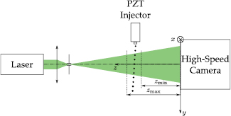
Figure 1. Experimental setup for holographic 3D tracking of free-falling droplets.
Download figure:
Standard image High-resolution imageAn example of a hologram obtained with the experimental setup shown in figure 1 is depicted in figure 2. As it can be seen, the contrast of the interference pattern is weak and the background is not spatially uniform. To avoid these problems, the acquired hologram sequences are pre-processed before being reconstructed.
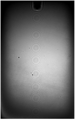
Figure 2. Example of an acquired hologram.
Download figure:
Standard image High-resolution image2.2. Holograms pre-processing
The aim of pre-processing the hologram is to enhance the signal to noise ratio (SNR) of the diffraction pattern. The principles of hologram pre-processing are illustrated in figure 3. Using the recorded hologram sequence, it is possible to build a background image by calculating the median of the sequence. Doing so makes it possible to obtain a background image with a noise structure much more representative of the hologram sequence than that of an 'empty' hologram recorded prior or after the image acquisition. For this purpose, the larger the number of acquired frames, the better the background. Here, all 1000 holograms were used to construct the background image. The constructed background image is then subtracted from the original hologram sequence, leading to an average removed sequence. It can be seen in figure 3 that the resulting sequence exhibits better fringe visibility and background uniformity. Moreover, the background noise (i.e. region of the hologram without interference signal) strongly resembles Gaussian white noise. This aspect will be very useful for the implementation of the proposed reconstruction scheme. This point is discussed in detail in section 4.
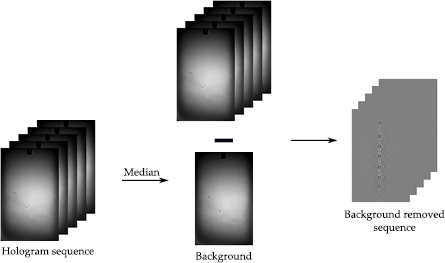
Figure 3. Pre-processing of the acquired hologram sequence.
Download figure:
Standard image High-resolution imageOnce the pre-processing step was complete, the hologram sequence is ready for hologram reconstruction. The proposed method is not based on backpropagation scheme as is often the case, but relies on inverse problem approaches. The next section is therefore devoted to the description of the reconstruction scheme.
3. Hologram reconstruction using inverse problems approaches
Standard hologram processing methods are based on light back-propagation methods [6]. These aim to calculate the Huygens–Fresnel integral from the recorded hologram giving the intensity of the light field in the object plane [37]. However, as these back propagation methods do not account for signal sampling, they are prone to ghost images [38]. In addition, as far as the in-line holographic configuration is concerned, reconstructed holograms are subject to twin-image disturbances, which drastically reduce the signal to noise ratio (SNR) of the reconstructed image, thereby reducing tracking accuracy. To overcome these problems, rather than back-propagating the hologram, an inverse problems (IP) reconstruction scheme can be considered [18, 22, 24, 39]. Assuming additive white Gaussian noise, the aim of this approach is to find the imaging model that best fits the experimental data, in the least-square sense. In our experimental configuration, a parametric imaging model relying on four parameters ( , see equation (4) for details) was available, and hence a parametric IP reconstruction [18, 22, 24]. Note that astigmatism, which can occur in pipe flow studies, can also be accounted for in the image formation model [40]. Tilt or spherical aberration can also be considered, leading to more complete image formation models. For more complicated objects or configurations a Maximum A Posteriori approach (MAP) [39, 41, 42] can be applied. All these approches, often referred to as compressive sensing [19–21], have been shown to lead to optimal signal reconstruction [16, 25].
The reconstruction algorithm used for this tracking study is shown in figure 4 and relies on two main steps:
- (i)
- (ii)

Figure 4. Schematic diagram of the reconstruction procedure used for high resolution particle tracking.
Download figure:
Standard image High-resolution imageIn the remainder of this article, this reconstruction scheme is applied to the tracking and particle sizing of a free-falling water droplet jet. Joint reconstruction with refined estimation of the radius r, is made possible considering r constant over each trajectory or at least over each hologram stack. It should be noted that this procedure can be generalized to other imaging techniques, and therefore not limited to holographic imaging, as long as a parametric imaging model is available.
4. Experimental results and data statistics
The experimental setup presented figure 1 is used for the holographic acquisition of free-falling water droplets injected with a PZT-injector. This injector can generate mono-dispersed droplets. Our joint reconstruction approach is expected to allow accurate estimation of the injected droplet radius. It should be noted that for a known noise model, the accuracy of the 3D positions of the droplets is driven by the Cramer–Rao lower bound [16] and can be as low as one hundredth of a pixel. Note that the main purpose of this experiment is to validate the performances of our reconstruction algorithm on bench-top experiments.
4.1. Accuracy of the droplet 3D tracking
Tracking is performed on a sequence of N = 1000 holograms. In order to reduce the data processing time, values of z and r will be optimized in a range of ±10% around roughly estimated values. More generally, the reconstruction approach remains valid as long as our imaging model remains valid (i.e.  ). Seven to eight particles can be tracked on each hologram. For statistical reasons, only particle trajectories that span at least 200 holograms were considered. Moreover the holograms are cropped in order not to consider objects that exit from the injector (these are not spherical and do not corresponds to our image formation model). Therefore, according to the acquired holograms,
  trajectories will be processed. For each trajectory, random stacks of
  holograms are built for the purpose of joint optimization.
An example of a hologram sequence is shown in figure 5(a) (see Media 1 for the dynamic sequence (stacks.iop.org/MST/27/045001/mmedia)). Here, white crosses corresponds to the position of the object detected using the first main steps of the reconstruction algorithm (i.e. classical IP reconstruction). A three-dimensional representation of the  is plotted in figure 5(b). The coordinates
  corresponds to the center of the hologram, while the injector is positioned at the top of the hologram (see figure 5(a)) and in the top left hand corner of figure 5(b). As it can be seen in figure 5(b), the extracted 3D trajectories are only weakly dispersed in both x and z directions. This can be explained by the fact that the imaging sensor is positioned to record the region of droplet injection, limiting the effect of the experimental environment on the droplet trajectories. To assess the accuracy of the 3D trajectory reconstruction, second order polynomial trajectories were fitted to the experimental data [43]. This choice was driven by the free-falling nature of the droplets. Results obtained for the
  trajectories are given in table 1 in the 3rd to 5th columns for the classical IP, and in the 7th to 9th columns for joint reconstruction. From these results, it can be seen that the joint reconstruction process weakly influences the accuracy of the 3D tracking. This result was to be expected as neither xi, nor yi, nor zi are constant throughout the image sequence. Moreover, it shows the low correlation between r and the
  parameters. It should be noted that the average processing time for each trajectory (classical IP approach and joint IP reconstruction for 8 particles tracked over 1000 holograms) is 8 h using Matlab 2015b on a high-end labtop computer (Windows 7-64 bit, Intel Core i7 3740QM @2.7 GHz with 24 Go RAM).

Figure 5. Example of particle tracking. (a) Parallel tracking of each particle in the hologram (full video sequence is available in Media 1 (stacks.iop.org/MST/27/045001/mmedia)). (b) Extracted 3D-trajectories for all the objects detected.
Download figure:
Standard image High-resolution imageTable 1. Data statistics for particle tracking and size estimation using both IP reconstruction and joint reconstruction.
| Tracka |  |
 |
 |
 |
 |
 |
 |
 |
 |
 |
 |
|---|---|---|---|---|---|---|---|---|---|---|---|
| 1 | 235 (26) | 0.11 | 0.14 | 19.64 | 0.26 | 16.8 | 0.11 | 0.13 | 16.39 | 0.052 | 10.3 |
| 2 | 321 (35) | 0.08 | 0.23 | 17.66 | 0.29 | 16.6 | 0.08 | 0.21 | 22.24 | 0.039 | 6.6 |
| 3 | 389 (43) | 0.10 | 0.37 | 15.61 | 0.27 | 13.9 | 0.10 | 0.37 | 21.29 | 0.035 | 5.4 |
| 4 | 459 (51) | 0.28 | 0.52 | 19.69 | 0.26 | 12.3 | 0.28 | 0.57 | 19.18 | 0.049 | 7.1 |
| 5 | 512 (56) | 0.45 | 1.77 | 19.31 | 0.25 | 10.9 | 0.44 | 1.71 | 18.39 | 0.039 | 5.2 |
| 6 | 513 (57) | 1.13 | 6.61 | 24.09 | 0.25 | 11.1 | 1.13 | 6.61 | 16.42 | 0.039 | 5.1 |
| 7 | 503 (55) | 3.49 | 2.89 | 20.89 | 0.24 | 10.5 | 3.49 | 2.88 | 19.24 | 0.046 | 6.2 |
| 8 | 501 (55) | 7.75 | 7.06 | 20.88 | 0.24 | 10.4 | 7.75 | 9.11 | 19.78 | 0.047 | 6.4 |
| 9 | 505 (56) | 7.45 | 8.76 | 21.79 | 0.26 | 11.5 | 7.57 | 10.13 | 23.14 | 0.041 | 5.4 |
| 10 | 507 (56) | 7.29 | 11.35 | 20.83 | 0.25 | 11.3 | 7.42 | 12.69 | 19.13 | 0.043 | 5.8 |
| 11 | 504 (56) | 6.16 | 6.71 | 19.38 | 0.24 | 11.0 | 6.16 | 6.75 | 19.76 | 0.031 | 4.2 |
| 12 | 478 (53) | 4.21 | 4.43 | 20.96 | 0.19 | 8.9 | 4.29 | 4.68 | 21.42 | 0.034 | 4.7 |
| 13 | 407 (45) | 2.84 | 2.95 | 18.33 | 0.11 | 5.6 | 2.91 | 3.03 | 22.63 | 0.031 | 4.5 |
| 14 | 338 (37) | 1.43 | 1.54 | 20.64 | 0.12 | 6.8 | 1.48 | 1.98 | 26.06 | 0.024 | 4.1 |
| 15 | 264 (29) | 3.54 | 3.94 | 21.29 | 0.13 | 8.2 | 3.54 | 3.87 | 25.56 | 0.037 | 7.1 |
aStandard deviations on the x, y, z particle positions  are estimated by fitting a theoretical free-falling droplet trajectory.
b
are estimated by fitting a theoretical free-falling droplet trajectory.
b corresponds to the number of hologram per trajectory.
cEstimated over the number of holograms of the trajectory.
dEstimated over the number of hologram stacks for each trajectory as given.
corresponds to the number of hologram per trajectory.
cEstimated over the number of holograms of the trajectory.
dEstimated over the number of hologram stacks for each trajectory as given.
This processing time can be improved through parallel processing strategies. Nevertheless, these discussions fall out of the scope of this article. According to the values listed in table 1, the tracking precision (assumed to be the standard deviation between estimated positions and the fit of the trajectory, under the assumption of a second order polynomial trajectory [43]), is found to be  μm3, corresponding to
  pixels. It should be noted that we do not assess the absolute particle position (note that theoretical localization accuracy can be as low as one hundredth of a pixel [16]) but the precision of the trajectory fit.
4.2. Accuracy of the estimation of the droplet radius
As the radius is assumed to remain constant over the hologram sequence, its estimate should benefit from our joint reconstruction approach. The accuracy of our radius estimation will be assessed by two quantities: the standard deviation of the estimated radius distribution  , and the standard error of the mean
  . From the standard deviations of both IP and joint reconstruction estimation of the radius
  , and
, and  , standard errors of the mean are defined as
for the standard error of the mean of r estimated by classical IP reconstruction. Here  is the number of holograms per trajectory. The standard error of the mean (used to assess the accuracy of the estimation of the average) of the radius estimation using joint reconstruction is given by
where  is the integer part of the ratio of the number of holograms per stack to the number of holograms per trajectory.
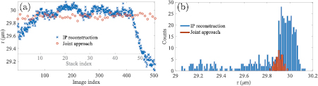
The statistical results of the estimation of the radius using the two reconstruction schemes are listed in table 1. In addition, to better underline the interest of our joint reconstruction approach, changes in the radius estimation and statistical distribution of the droplet radius are illustrated in figure 6. These graphical representation were performed considering the 11th trajectory. In both figures 6(a) and (b), results obtained with classical IP reconstruction are plotted in blue, while results obtained with the joint reconstruction approach are plotted in orange. The interest of the random hologram stack construction is clear in figure 6(a). As can be seen, the estimated values of the radius are biased at the end of the hologram sequence and noise is clearly visible on the estimation. This behavior is no longer noticeable in the joint reconstruction results where the estimated values are barely scattered around the average estimate. This point is confirmed by the statistical distribution in figure 6(b). The results for all the trajectories are given in Media 2 (stacks.iop.org/MST/27/045001/mmedia). Note that estimates of the radius are less dispersed around the distribution average when a joint reconstruction scheme is used.
Figure 6. Evolution of the estimated radius in trajectory 11. Results obtained for classical IP reconstruction are in blue, the joint reconstruction estimates are in orange. (a) Evolution of the radius as a function of the image/stack index. (b) Statistical distribution of the estimated values of the radius (Histogram for all the trajectories are given in Media 2 (stacks.iop.org/MST/27/045001/mmedia)).
Download figure:
Standard image High-resolution image
Results obtained for the 15 tracks are summarized in table 1. From these 15 independent trajectories, and considering that the injector generate monodispersed droplet distributions, we can estimate the average standard deviations and standard errors for the two reconstruction methods. As the number of holograms differs from one trajectory to the next, weighted average values are calculated considering
for the classical IP reconstruction, and
for the joint reconstruction. Weighted averages on the standard errors were obtained the same way.
Therefore using classical IP reconstruction the radius can be estimated with a standard deviation  μm and a standard error
  nm, while using a joint reconstruction scheme these values are
  μm and
  nm resulting in a gain of 5.9 on the standard deviation and 1.9 on the standard error. It should be noted that in the case of white Gaussian noise, if the estimation of the radius computed using classical IP were averaged over
  holograms instead of performing the joint estimation reconstruction, the maximal gain in the radius estimation would be
  , which is half of the gain obtained using our method. Compared to a classical back-propagation reconstruction approach, the IP method has been shown to result in an improvement of the 3D localization of parametric objects [22]. As our approach is based on model-fitting, single point resolution has to be considered [16]. However, two-point resolution (e.g. Rayleigh criterion) is often considered.
For the purpose of comparison, and according to our experimental conditions, the Rayleigh criterion gives  μm, and
  mm considering a numerical aperture of
  , which are 40 times higher for lateral resolution and 300 times higher in axial resolution.
4.3. Discussion about image formation model
Despite their consistency, the presented results can be biased by an inadequacy of the imaging model used for hologram reconstruction. To test the validity of our model, we performed particle hologram simulations with an electromagnetic model (Lorenz–Mie theory). Comparison with our simplified imaging model shows a difference of less than 2% in intensity. To estimate the bias thus introduced, simulations are realized under realistic conditions (parameters corresponding to our experiments, addition of a white Gaussian noise with the same variance as that of figure 5(a)). Reconstruction of the simulated holograms is realized using IP reconstruction with the Tyler/Thompson image formation model (see [36]). From the processing of these holograms, the bias introduced by the simplified model, is found to be about 1.5% on the z, r parameters estimation, while x, y estimation is not affected. This point shows the limits of our approach using a simplified model. Let us note that the whole process is 10 times longer using a Lorenz–Mie model due to its computation complexity. However this model can be used in a calibration step for the estimation of the reconstruction bias, making it possible to unbias measurements. These results were obtained in the particular case of digital in-line holography with parametric objects. It should however be noted that more complicated objects can be considered using a regularized MAP reconstruction approach. Moreover, the proposed method is not limited to digital in-line holography but can be generalized to any technique that is based on a reliable physical model.
5. Conclusion
Digital in-line holography was successfully applied to the 3D-reconstruction and sizing of a free-falling water droplet jet generated by a PZT-injector. Instead of transforming data through Fresnel based light back-propagation calculations, holograms were processed using IP reconstruction. This method makes it possible to obtain 3D position parameters as well as the size of the droplets being investigated. Moreover, by exploiting the information redundancy of a temporal acquisition of holograms, it is possible to improve estimation of at least the parameters that remain constant during the acquisition.
Based on this principle, a joint estimation reconstruction scheme was developed. Accurate estimation of the 3D location of the droplets was intrinsically provided by the classical IP reconstruction algorithm, while the precision of the droplet size parameters was improved by jointly estimating their value over randomly built hologram sequences. This method proved to be less sensitive to measurement biases than the classical IP reconstruction, making it a method of choice for both high resolution tracking and particle sizing.
The proposed joint reconstruction scheme makes it possible to reconstruct a 3D droplet jet with a precision of  μm3 over a field of view of
  , and also makes it possible to achieve a droplet sizing precision of
  μm with a standard error
  nm. This results in a gain of a factor 5.9 in standard deviation and 1.9 in standard error compared to classical IP reconstruction. Considering the low standard deviation values achieved, cares are to be taken about the choice of the model to prevent from reconstruction bias.
The proposed method can be used for every imaging technique associated with a known imaging model and can be advantageously used for accurate estimation of redundant parameters in image sequences (e.g. optical properties, mechanical properties...).
Acknowledgments
The authors are grateful for the financial support of Université de Lyon through the Program 'Investissements d'Avenir' (ANR-11-IDEX-0007), and LABEX PRIMES (ANR-11-LABX-0063). The authors also would like to thank the French National Research Center (CNRS) for supporting this research work through the project DETECTION funded by the call for projects DEFI IMAGIn 2015.