


Abstract
A novel angular resolved scattering system for measurements of spatial angular distribution function (3D ADF) of scattered or emitted light using a digital camera is presented. 3D ADF is determined from the digital image captured from a transmissive flat screen. With the developed camera-based system we can quantify transmitted or reflected light scattered by textured samples or emitted light from light sources in a few seconds. In this paper the setup of the camera-based system is described, and the main transformations of the acquired digital image to obtain the 3D ADF are explained, along with the haze calculation. The system is applied and validated on a randomly nanotextured transparent sample and a periodically textured non-transparent sample. Good matching is obtained with rigorous simulations and measurement results carried out with a conventional goniometric angular resolved scattering system.
Export citation and abstract BibTeX RIS
1. Introduction
Light scattering is an important phenomenon in a broad range of applications, in particular for efficient in-coupling or out-coupling of light in photovoltaic and optoelectronic devices [1]. Scattered light is usually induced by nanorough surfaces in the device. In solar cells, scattered light rays have prolonged optical paths, ultimately resulting in higher conversion efficiency. In the case of light sources, scattering at nanorough surfaces is used to broaden the angular distribution of emitted light. As different (nano)structures scatter light differently, it is of great importance to know and quantify the process of light scattering. The basic concepts of light scattering measurements are therefore standardized and described in ASTM [2, 3] and ISO [4] standards.
In the field of (thin-film) photovoltaics, two main techniques are used to characterize light scattering properties of rough surfaces: total integrating scattering (TIS) and angular resolved scattering (ARS). TIS measures the entire scattered light and does not include the directional (angular) information on scattered light [5]. Using a monochromator and an integrating sphere with openings, TIS measurements are performed in a broad wavelength range for both reflected and transmitted light.
In the case of ARS, goniometric based systems are used to measure angular distribution function (ADF), usually in one plane only (1D ADF). Different goniometric ARS systems have been developed, such as ones by Rifkin et al [6], Krč et al [7], Schröder et al [8], Amra et al [9] and Jäger et al [10] where the last two can measure ADF in a broader wavelength range. Since they usually use a goniometric scanning method, ARS systems are quite time consuming even if measuring in one plane only. In case of random textured surfaces, assuming rotational symmetry, one plane provides enough information to predict the intensity distribution in 3D space. However, goniometric scanning is not time-effective and sometimes not sufficient to accurately determine light scattering in 3D space. In order to acquire more complete information about 3D ADF in a short time, camera-based ARS systems are used. Some of them are commercial products [11, 12]. For light sources, hemispherical reflective screens are typically used that are already fully compliant with standards. Scattered light can also be projected onto flat screens that are either reflective or transmissive.
A few camera-based systems used at laboratory scale have already been reported. Berner et al [13] introduced a system with a lens and transmissive screen for measurements of transmitted scattered light. In our previous publication [14], we reported on a system where we included the lens to broaden the polar angle range. However, a reflective screen was used instead of a transmissive one in order to gain in the signal. A similar approach (but without a lens) was used for the characterization of optical films for 3D displays [15]. Foldyna et al [16] reported on a system for spatial measurements of reflected light in a broad range with a very complex conoscopy configuration. Some other publications on the measurements of reflected light were also reported [17, 18]. They, however, have been developed for applications (road surface reflectivity and modelling for computer graphics, respectively) and samples that are very different to the application and samples discussed here. Additionally, light scattering systems were built to analyze reflection under illumination from linear light sources [19] and inspect surface roughness or defects [20–22].
In this paper we present a novel camera-based ARS system. Due to its speed, the 3D ADF is measured in a few seconds compared to from 0.5 to a few hours (depending on the requested resolution) with goniometric systems, the developed system is suitable for in-line or off-line quality control in production monitoring. In the setup we use a transmissive screen, positioned non-perpendicularly at the specular beam to cover large scattering angles. Compared to the other reported setups, such configuration enables measurements of all the polar angles θ, from 0° to 90°. To broaden the range for azimuthal angles φ, we apply a few step rotations of the sample and/or the screen with the camera. Our camera-based system is useful for both scattering samples and light emitting samples (LED and OLED). Besides transmitted, the new setup enables also measurements of reflected light which has not been reported yet. In addition to the fast and accurate determination of the (full) 3D ADF, we will show how to obtain the haze parameter (ratio between integrated diffused over total light) with the new setup. We also carried out basic repeatability and uncertainty analysis.
In the first part, we will present the configuration of the system and image processing procedure to acquire light scattering parameters of the sample from raw image. In the results section we will present the results of measurements of the two selected samples: nanotextured transparent conductive oxide on a glass substrate and periodically textured silicon sample. The results of the haze determination will also be shown.
2. Experimental
2.1. The setup
The setup of the novel camera-based system is illustrated in figure 1. A collimated laser source with a selected light wavelength is used to illuminate the sample. A collimated light from a monocromator can be used if a scan over the wavelength range is needed. The scattered or emitted light from the sample is projected on the transmissive screen and captured by the camera. The screen, positioned at α = 45° to the sample plane, is used for either reflectance or transmittance measurement, denoted with R and T in figure 1. When measuring the reflected light, the laser beam is first let through the hole in the screen R so that it can reach the sample. When measuring the transmitted light, the specular beam needs to be blocked with a pin on the screen T if it causes camera saturation and/or blooming effect. A hole could also be used instead of the pin. However, when measuring specular beam the hole would have to be filled with the screen material. To capture the image from a screen, a 1.4 Mpixel CCD camera with 16-bit resolution was utilized in our system, positioned perpendicularly to the screen(s). This way we avoid additional asymmetry transformations.
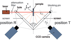
Figure 1. Schematics of the camera-based system for measurements of reflected and transmitted light. The screen angle α = 45°. In case of measurement of reflected light, the laser beam is let through the screen via a hole in the screen. In case of a measurement of the transmitted light, the specular beam is blocked to prevent camera saturation. The camera captures the light that is projected on the screen. Attenuation filter position is also depicted, as it will be later referenced in the haze results section.
Download figure:
Standard image High-resolution imageIn figure 1 two configurations are presented, one for reflectance (position R) and one for transmittance (position T). It requires two cameras and two screens to measure scattered light in R and T simultaneously. In case of a single camera, an automatic (or manual) rotation of 90° is needed to change the camera from one position to the other, allowing us to sequentially measure both R and T. Due to possible reflections from one screen onto another, additional care is advised.
With the placement of the screen as shown in figure 1, we do not cover the entire hemisphere of reflected or transmitted light, but only a part of it. This way, however, we get full polar range θ, from 0° to 90°, at the cost of a smaller azimuth range. The range can be extended to almost a full sphere (in R or T) by, for example, rotating the camera around the sample for 90°, 180° and 270° or, as will be proposed here, by rotating the sample. Nonetheless, if samples scatter light isotropically, one measurement is sufficient and can be extended to other azimuthal angles considering rotational symmetry.
2.2. Image processing and transformations
Once the image from the camera is captured, it needs further processing and transformations to acquire the correct 3D ADF from its pixel values. Camera effects, such as noise offset and outliers, have to be removed first. Furthermore, to gain comparable results from different measurements, the intensities of the pixels in the images are normalized with their integration time as the used camera has linear time dependency. Here we follow standard procedure, as described in [23]. In cases where the light source intensity changes, the pixel intensities need to be normalized once more.
2.2.1. Coordinate system.
In our transformations and 3D ADF presentations we will refer to the spherical coordinate system as presented in figure 2. Symbol θ denotes the polar angle and φ the azimuth angle. The origin of the spherical coordinate system is set at the illumination point of the laser beam on the sample.
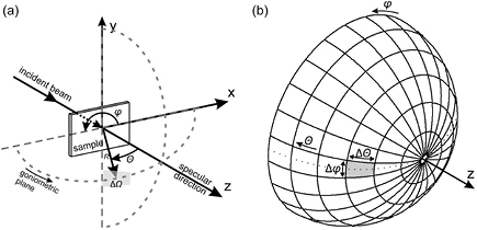
Figure 2. (a) Coordinate system for the camera-based system. Spherical and Cartesian coordinates are denoted together with specular direction. A selected solid angle area ΔΩ for 3D ADF in transmission is presented. A goniometric plane is drawn for further reference. (b) A hemisphere with lines with constant Δθ and Δφ. Spherical coordinates θ and φ are shown together with z as specular direction. The goniometric plane is presented with a dotted line.
Download figure:
Standard image High-resolution imageDespite the angular distribution of scattered light being a continuous function in general, a discrete representation of the ADF at the specific angles is widely accepted and applied also in our case. The 3D ADF is here defined as a light intensity in a discrete solid angle ΔΩ =  . We measure it at a certain distance from the sample (in the far field region). A solid angle ΔΩ at the specific coordinates θ and φ, is also depicted in figure 2. Figure 2(b) presents a hemisphere where lines with constant Δθ = Δφ = 15° are shown. It is noticeable that over the sphere the areas with constant Δφ and Δθ are different, therefore they have different ΔΩ. For a valid presentation of the 3D ADF, the ΔΩ should remain constant over the sphere. To ensure the same ΔΩ at each coordinate, the Δθ should stay the same, but Δφ has to be weighted with
  following the solid angle formula.
When presenting the 3D ADF, our discrete spherical coordinate system is defined with the angular step of 1°: θi = 0°, 1°, 2°...90° and φi = 0°, 1°, 2°...360° to cover the whole (hemi)sphere, while the same ΔΩi was set with Δθ = Δφ = 0.5° and appropriate  .
.
Below we show the image transformation procedure for the transmission case (position T in figure 1). The procedure for reflection, however, is the same, just for the other hemisphere.
2.2.2. Angle transformation/determination.
The scattered light is projected on the screen which is flat and not hemispherical, therefore the same ΔΩ covers different areas on the screen for different θi and φi. The following procedures have to be carried out to ensure that the scattered light intensity at a chosen spherical coordinate corresponds to the same solid angle ΔΩ and its projection on the screen. First, central points of each of the pixels from the image are positioned in a spherical coordinate system:

Indices m and n determine lateral and vertical positions in a pixel matrix (m = 1...1040, n = 1...1392, 1.4 Mpixel camera). Second, pixels with central point coordinates within a certain ΔΩ region are summed. The scattered light intensity in a certain ΔΩi at a chosen spherical coordinate (θi, φi) is therefore proportional to the sum of pixel intensities Ipixel within the ΔΩi:
2.2.3. Screen characteristics.
It is of key importance to use highly transmissive and diffusive screens in order to assure a sufficiently large signal in the case of samples with low scattering levels. The diffusive nature of the screen enables that each of the illuminated points on the screen directs a portion of light towards the camera. From the point of view of the transformation, the ideal light scattering distribution of the screen—the ADF of the screen, ADFscreen—would be uniform, i.e. equal intensity in all scattering angles and independent on the incident angle of illumination ray. As this is not the case, the ADFscreen has to be known or determined in advance.
In our case two isotropic diffusive screens were used: (a) opal diffusing glass (25 × 30 cm2) [24] and (b) PLEXIGLAS® (21 × 30 cm2) [25]. RTA measurements in a broad wavelength range were conducted for both screens, the results are presented in figures 3(a) and (b). Both screens have around 30% transmission at λ = 633 nm (later used in measurements), such transmission is sufficient for camera-based measurements. At longer wavelengths, the PLEXIGLAS® has higher transmission, making it more suitable for NIR measurements. Optical losses of transmissive screens are presented by reflected light and internal absorption losses in figures 3(a) and (b). Low reflection is desired as the reflected light can reach the sample and distort the measurements. This, and the size of the screen, has to be considered when choosing the distance between the sample and the screen.
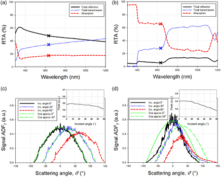
Figure 3. RTA measurements of (a) opal diffusing glass and (b) PLEXIGLAS®. Goniometric ARS measurements of ADFT in a plane at λ = 633 nm for (c) opal diffusing glass and (d) PLEXIGLAS® at selected incident angles. Cosine approximations for angles 0° and 30° were added. Amplitude peaks (after interpolation) dependent on incident angle for opal diffusing glass and PLEXIGLAS® are also shown as inserts in top right corner in (c) and (d), respectively.
Download figure:
Standard image High-resolution imageFor both screens ADF in transmission ADFTscreen in a horizontal plane −90° < θ' < 90° was measured with the goniometric ARS system, isotropy of the screens was assumed. The incident angle of the 633 nm laser beam towards the screen was altered between 0° and 60° with a step of 5° to acquire all the needed data, the results for selected incident angles are presented in figures 3(c) and (d). Compared to the PLEXIGLAS®, the opal diffusing glass exhibits almost perfect cosine (Lambertian) distribution (the cosine approximation is also plotted as a reference). With increasing incident angle a peak amplitude drops (see inserts top right corner in figures 3(c) and (d) and angle shift can be observed.
As shown, different screens have different ADFs, so ADFTscreen needs to be included in the image processing procedure. First, for each ΔΩi (summation area) the resulting average incident angle γin of the scattered rays from the sample to the screen is calculated based on the system configuration. Second, for the same ΔΩi exiting angle γex from the screen towards the camera is also calculated. Both angles are denoted in figure 1. The γin is used to select the appropriate ADFTscreen curve while γex defines the scattering angle of the screen. The intensity I'(θi, φi) of each ΔΩi is then weighted with the obtained value. Finally, the correct scattered light intensity, equal to ADF, is therefore:

The screen thicknesses for opal diffusing glass and PLEXIGLAS® are 3 and 5 mm, respectively, the refractions inside the screen can be and are neglected in the calculations.
As both screens are commercially available and intended for general purpose usage, such as rear projection, no polarization effects due to the screens were expected or observed in our system. By putting a polarization filter after the light source or the sample, one is also able to measure the scattered polarized light with the camera-based system [15].
2.2.4. Image processing in graphics.
As a conclusion to the image processing section, the discussed transformations parameters are graphically shown for the system configuration described in the results section. Figure 4(a) shows the number of pixels summed per summation area, determined by Δθ = 0.5° and Δφ = 0.5°. The amount increases as we move outwards of the perpendicular direction to the screen, (θ, φ) = (45°, 180°) where the projection of the solid angle area on a (flat) screen surface is the smallest. Just around the origin of the coordinate system, the amount of summed pixels is the highest due to the azimuth angles being so congested (see figure 2(b) around specular beam). Figure 4(b) shows PLEXIGLAS® screen weight function that can be composed from the ADFTscreen values. The peak is again at perpendicular incident angle on the screen, (θ, φ) = (45°, 180°), outwards of this peak the value decreases, resulting in a higher value of the ADF after weighting. Both figures show vertical symmetry (φ = 0°, 180°). The edges of the graphs (coloured, signal area) are determined by the camera angle of view (shape of the sensor), defining the range of the single measurement. These matrices are dependent on the system configuration (distances between the elements), camera resolution and screen, not on the sample, and can therefore be considered as a constant for the individual system setup configuration.
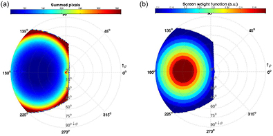
Figure 4. (a) number of summed pixels per summation area (θi, φi) and (b) screen weight function (θi, φi) for PLEXIGLAS®.
Download figure:
Standard image High-resolution image2.3. Haze determination
Besides the determination of the ADF we also tested whether our system can be applied to determine the haze parameter based on the ADF measurements. This requires the measurement of the specular component of the light which presents a challenge and also affects the accuracy of the haze determination procedure [10]. In this section we will show how to calculate it for the case of transmitted light, the same procedure can be followed for the reflected light (substitution of T with R, slight sample rotation is needed so that the specular beam can be caught on the screen instead of passing back through the hole). Our approach to the measurements of the specular component will be described in the results section. Haze in transmission is defined as [5]:

where ITdif and ITtot are diffuse and total light scattering intensities. When used in a ratio we can describe haze with diffuse and total (Tdif and Ttot) transmittance, where Ttot consists of diffuse and specular (Tspec) parts. This means measurements with the camera must be in our system performed without a blocking pin on screen to capture the specular part. However, camera saturation must be avoided (see section 3.2). The values for Tdif and Tspec are in general obtained by integrating the diffuse and specular light over the hemisphere [10]:

The symbol θi denotes the boundary angle between the specular and diffuse part. In case of light scattering by isotropic sample, the azimuth component can be neglected and the integrals can be simplified into the following auxiliary equations:

ADF1D is the average line and is extracted by averaging the 3D ADF for each θ through all φ that we measured with the system. ADF1D is then transformed to ADF3D where we expand the line over the whole hemisphere [5]. Δθ was set at 0.5°. Specular beam value (SBV, θ = 0°) in ADF3D is 0 because of the cosine part, therefore we calculate SBV by summing all the azimuth values for polar angle θ = 0° and weighting it with the solid angle a beam with 2* Δθ = 1° would cover. The specular and diffuse components are then calculated as following:

3. Results and discussion
The applicability of the presented system is demonstrated with two different light scattering samples: for transmittance measurements we selected a textured transparent conductive oxide (TCO), used as a substrate in thin-film solar cells, and for reflectance a periodically textured silicon sample. The SEM images of the tested samples are shown in figure 5.

Figure 5. SEM images of (a) textured TCO—magnetron sputtered ZnO:Al, etched in HCl for 30 s and (b) for periodic hexagonal hole array with a period of 1500 nm and depth of 550 nm on silicon substrate. Main planes of the sample are drawn for further reference (a = 750 nm and b = 1299 nm).
Download figure:
Standard image High-resolution image3.1. 3D ADF
For the measurements presented below, the distance between the sample and the screen was set to 11.4 cm in specular direction (direction of the laser beam) to avoid strong reflection relation between the screen and the sample. The distance between the screen and the camera was 35.7 cm so that all polar angles could be captured with our camera. HeNe gas laser with a λ = 633 nm and P = 10 mW was used in the measurements. Other lasers/wavelengths can also be used, with screen characteristics (ADFTscreen) accordingly applied. The samples were perpendicularly illuminated. Normally, camera integration time varies between 0.5 and 2 s, depending on scattering abilities of the sample, the power of the laser and the screen used. All the images are therefore time normalized to gain comparative results.
First, we show the result of 3D ADFT for magnetron sputtered ZnO:Al, etched in HCl for 30 s, exhibiting crater like random texturization with vertical root-mean-square roughness of ~110 nm [26]. PLEXIGLAS® was used as a screen here. Figure 6(a) shows raw image as captured with the camera before any processing, camera integration time was t = 0.25 s. Quasi-elliptic bright area and dark black spot, where the pin blocks the specular beam, can be observed. After applying the transformations described in section 2.2 an expected circular pattern (rotationally symmetric isotropic scattering) is acquired (figure 6(b)). A much lower signal at the position of the specular beam (0, 0) is a result of a pin blocking the specular beam. This figure also shows the available range of the single measurement (M1) of the setup for the selected distances between the elements, which is 0° < θ < 90° and approximately 130° < φ < 230°. Confined by the rectangular shape of the camera sensor (before the image processing), the polar angles increase from 45° at φ = 90° (270°) to 90° at φ = 130° (230°).

Figure 6. Transmittance measurement results for ZnO:Al, etched in HCl for 30 s, for λ = 633 nm with PLEXIGLAS® as a screen: (a) image from the camera, (b) measured 3D ADFT, single measurement M1 (c) 2 measurements M1 + M2 combined where the sample was rotated for 180°. (d) Comparison between camera-based ARS and goniometric ARS. Red and green solid lines from (c) match those in (d). (e) Average line scan and standard uncertainty at each polar angle for the selected sample obtained from 12 measurements with PLEXIGLAS® as a screen. Comparison between the measurement results with both screens for three different TCO samples. The grey areas in (d), (e) and (f) show where the error due to the blocking pin and spike just after it is.
Download figure:
Standard image High-resolution imageGreater angular range can be obtained by, for example, one additional measurement by rotating the sample for 180° (M2) and recapturing the screen image with the camera; this is presented in figure 6(c). In this way, with our setup, only a minor part of the hemisphere was not measured (white/light grey area in figure 6(c)), but could be fully measured by additional rotation of the sample by 90° (M3) and 270° (M4). The lines denote the range of the individual measurement (M1, M2, M3 and M4) if all four measurements would have been performed. Nevertheless, rotational symmetry in the 3D ADF of the sample can clearly be observed with two and even one measurement.
To validate the system, a conventional goniometric ARS system was used as a reference, where the scattering in a selected plane (denoted in figure 2) perpendicular to the sample is measured. A scan from such measurement was compared with line scans at φ = 180° (M1) and φ = 0° (M2) from 3D ADFT and shown in figure 6(d). Besides the differences around angle 0° due to the blocking pin and the spike just after (the area where greater error appears was marked grey in figures 6(d)–(f)), good matching between both measurements is obtained. While the matching is not 100%, it is more than sufficient for the inspection systems in photovoltaics where fast throughput often prevails over accuracy.
For the selected sample and PLEXIGLAS® as a screen, we also investigated the uncertainty of the measurements. Twelve measurements were carried out under the same conditions, from which the average value and standard deviation at each scattering angle were calculated. The standard deviation was then used as a standard uncertainty. The results are shown in figure 6(e). The average values are presented as an ADF curve and the standard uncertainty with error bars. We can conclude good repeatability and low standard uncertainty of the measurement system, which, combined with the obtained good matching, validates the system.
To compare the performance of the two analyzed screens, the light scattering from three ZnO:Al samples with different etching times (30 s, 20 s and 10 s, rms values 110 nm, 90 nm and 50 nm, respectively) was measured using both screens. The line scans from the obtained 3D ADFT are compared in figure 6(f). Measurements with both screens result in very similar ADFs, making them both suitable for the ADF measurements if their characteristics are accordingly applied.
Second, reflection measurements will be presented on a case of a periodic hexagonal hole array on silicon substrate with a period of 1500 nm and depth of 550 nm (commercially available sample [27]). The system was also successfully calibrated by linear 1D gratings. However, compared to periodic 1D gratings, periodic samples with 2D hexagonal grating scatter light not only in one plane but in space. This makes them perfect candidates to show the advantage of the camera-based 3D measurement system which enables us to detect multiple spatially distributed modes with a single measurement. Following the diffraction grating equation, different modes at different polar angles can be calculated for the selected sample (table 1).
Table 1. Calculated modes for hexagonal hole array with a period of 1500 nm for λ = 633 nm.
| Mode order | Effective period, d (nm) | Notation on figure 5(b) | Mode angle, θ (°) |
|---|---|---|---|
| 1 | 1500/2 = 750 | a | 57.57 |
| 1 | 1500 *  /2 = 1299 /2 = 1299 |
b | 29.16 |
| 2 | 1500 *  /2 = 1299 /2 = 1299 |
b | 77.05 |
The mode angles for the inspected sample were calculated using the diffraction grating equation [28]:

Symbol θ denotes the scattering mode angle, m is the mode order, d is the period or as is the case with 2D gratings, the effective period as the distance between the planes rather than the period has to be considered. Two main effective periods, a and b shown schematically on SEM image in figure 5(b) with corresponding planes, were used in calculations. Incident wavelength λ = 633 nm in air was assumed.
Figure 7(a) shows the measured 3D ADFR of the periodic sample. Opal diffusing glass was used as a screen, camera integration time was t = 0.1 s. The measured modes are in good agreement with the calculated modes—the red lines with θ as calculated in table 1 were added to the plot. In addition, for this sample we simulated the 3D ADFR using combined FEM (finite element method) and Huygens expansion approach [29], providing the additional validation of the system (figure 7(b)).
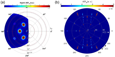
Figure 7. Reflectance of hexagonal hole array (period 1500 nm) for λ = 633 nm: (a) measured 3D ADFR and (b) simulated 3D ADFR. Opal diffusing glass was used as a screen, t = 0.1 s. In figure (a) red lines with θ as calculated in table 1 were added to the plot for validation.
Download figure:
Standard image High-resolution imageAs previously mentioned, all the measurements were carried out under perpendicular illumination. With the presented camera-based system, light scattering at different non-perpendicular illumination angles can also be measured. Since the non-perpendicular illumination will most likely cause an asymmetrical ADF pattern, both sides have to be measured rather than rotating the sample. Therefore the screen and/or camera have to be placed on the other side (rotated for 90°—manually or by rotating arm), with the camera looking perpendicularly at the screen and the screen angle being 45° at the sample at any illumination angle.
3.2. Haze
As a proof of concept, we present the haze obtained with our system for the three above mentioned ZnO:Al samples with different etching times (30 s, 20 s and 10 s), resulting in different hazes. PLEXIGLAS® was used as a screen for all the haze measurements. The diffuse part was measured exactly as described above in section 2.2 (normal, single measurement, t = 250 ms). The specular part, however, required additional measurements due to a strong specular component. The specular beam can exceed the scattered light intensity by a few decades depending on the scattering abilities of the sample and would in normal (ADF) measurement cause saturation of the camera. Therefore multiple images are needed to gradually measure the specular beam—the peak itself and the small area just around the peak. This way we get the signal to fill the black spot caused by the pin (see figure 6(a)) and obtain the correct value of the specular beam. If the used camera has higher resolution than ours (16-bit), single measurement may be sufficient.
The additional measurements of the specular part were performed without the blocking pin, but with an attenuation filter with 9.12% transmission at 633 nm and decreasing integration times of the camera (250 ms, 50 ms, 1 ms and 0.5 ms) to prevent camera saturation. All images were normalized with camera integration time and composed together. After the new full image was acquired, the haze was determined as explained in section 2.3. Following the results shown in figure 6, rotational symmetry was assumed for all three samples. Simplified equations for average line scan were correspondingly applied. The boundary angle θi was set to 4°, corresponding to the opening size in the integrating sphere.
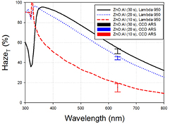
The haze results obtained from camera-based measurements were compared with measurements done with spectrophotometer Lambda 950 and are shown in figure 8. The haze scans with Lambda 950 were done in a broad wavelength range, while the camera-based haze determination was carried out at the selected wavelength λ = 633 nm. Three camera-based haze measurements were done for each sample, allowing us to also plot the error bar. The comparison shows moderate matching, with the highest discrepancies for the third sample (red colour). The system is primarily built for the determination of light scattering—diffuse part, ADF—for which it shows good accuracy. The main error in haze determination, however, is caused by the specular part. This could be due to the laser instability combined with extremely short camera integration times (0.5–1 ms). Even small errors can escalate when they are normalized by a couple of decades' different factors. Still, the results are good enough for the haze estimation. As mentioned above, they could be improved by using a camera with higher resolution.
Figure 8. Haze curve obtained with Lambda 950. Measurements with camera-based system are added at λ = 633 nm.
Download figure:
Standard image High-resolution image
4. Conclusions
The described camera-based ARS system enables fast and accurate measurements of light scattering properties of textured surfaces and light emitting devices with a single shot in a 3D space in broad angular range in a few seconds. We presented the solution which can be used for measurements of reflected or transmitted scattered or emitted light. The tilted screen position allows us to measure full polar range at the cost of the limited azimuthal range. However, with appropriate (automatic) rotation of the sample scattered light in full sphere can be obtained. Additionally, the system was also applied to the determination of haze parameter.
Measurements of two types of scattering samples were presented. Randomly textured ZnO was used to show how to acquire full sphere 3D ADF by rotating the sample. Characterization of periodically textured silicon substrate was used to demonstrate the advantage of using spatial (camera-based) systems instead of conventional goniometric systems. With one measurement we were able to detect all the modes of the periodic sample in the angular range of the measurement. The goniometric system, together with simulations, was used for validation of the newly developed system. Comparison with other methods showed good matching.
The presented camera-based ARS system is a powerful tool for optical characterization and can be applied also as an inspection tool in high throughput industrial production. Randomly, periodically and quasi-periodically textured transparent samples or light sources, such as LEDs, can be characterized accurately and in a very short time (seconds).
Acknowledgment
Miro Zeman and Olindo Isabella from Technical University Delft are acknowledged for providing TCO samples. The authors thank Martin Sever for carrying out the simulations. The authors acknowledge the financial support from the Slovenian Research Agency (program P2-0197 and project J2-5466). MJ thanks the Slovenian Research Agency for his PhD funding.