


Abstract
The behavior of a bubbly two-phase flow in the vicinity of a wall affects heat, mass, and momentum transfer; therefore, there is great interest in developing a quantitative technique to monitor this behavior. Herein we propose a new method based on ultrasound echo signal processing that it feasible for industrial applications where the boundary layer is modified by traveling bubbles. By introducing time-resolved direct waveform analysis at 100 MHz, we have succeeded in the spatio-temporal detection of bubble surfaces at echographic profiling frequencies in the range of 15–20 kHz. Unlike conventional approaches, which use short pulses, a relatively long pulse length is applied to allow ultrasound Doppler velocimetry in the liquid phase. Examination of the horizontal bubbly two-phase turbulent channel flows demonstrated the feasibility of this method; spatio-temporal echography of moving bubble surfaces is successfully achieved as the bubbles travel on length scales smaller than the spatial ultrasonic pulse length near the wall. The applicable range of parameters (e.g. bubble size and shape, and flow speed) was determined by 3D numerical analysis of the wave equation and its application to bubbles flowing beneath a flat-bottom model ship.
Export citation and abstract BibTeX RIS
Nomenclature and units
| a, b | long and short lengths of a spherical bubble, m |
| B(t) | echo signal from the bubble surface, Pa |
| cw | speed of sound in water, m/s |
| DU | diameter of the ultrasonic beam, m |
| DB | size of the bubble, m |
| dB | distance between the wall and bubble surface, m |
| fr | pulse repetition frequency, Hz |
| fs | sampling frequency, Hz |
| fU | ultrasonic frequency, Hz |
| H | height of the model ship, m |
| h | half height of the channel, m |
| L | length of the model ship, m |
| Ld | distance from the center of the bubble to the center of the ultrasonic beam, m |
| Lp | pass length of the ultrasonic beam, m |
| Lx, Ly, Lz | distance in each direction for a region of the numerical simulation, m |
| n | number of cycles in the ultrasound pulse, dimensionless |
| P | acoustic pressure, Pa |
| P0 | maximum emitted acoustic pressure, Pa |
| PB | maximum echo amplitude from the bubble surface, Pa |
| PM | maximum echo amplitude, Pa |
| Pr | acoustic pressure received by the receiving ultrasound transducer, Pa |
| PW | maximum echo from the upper wall, Pa |
| Reh | Reynolds number defined by the half height of the channel, dimensionless |
| Rex | Reynolds number on the flat plate, dimensionless |
| S(t) | echo signal from the wall and bubble surface, Pa |
| tdelay | time for a round trip of ultrasonic pulses in the liquid film, s |
| t | time, s |
| Ubulk | bulk mean velocity of the test flow, m/s |
| Uship | main flow velocity under the ship (equivalent to towing speed), m/s |
| uB | advection velocity of the bubble surface, m/s |
| uy | streamwise velocity distribution in the turbulent boundary layer, m/s |
| V | echo amplitude, V |
| VM | maximum echo amplitude near the upper wall, V |
| VW | maximum echo amplitude from the upper wall, V |
| W | width of the model ship, m |
| W(t) | echo signal from the wall, Pa |
| x, y, z | x, y, z coordinates in the experimental setup, m |
| xʹ | streamwise length from the measurement point, m |
| Δxʹ, Δy | spatial resolution in the x and y directions of the ultrasonic measurement, m |
| Zmaterial | acoustic impedance of the material, kg/m2 s |
| αchannel | void fraction in the channel flow, dimensionless |
| αδ | void fraction in the turbulent boundary layer on the flat plate, dimensionless |
| Γ | oblateness of a spheroidal bubble, dimensionless |
| δx | 99% turbulent boundary layer thickness, m |
| λ | wavelength of the ultrasound, m |
| ν | kinematic viscosity of the test fluid, m2/s |
1. Introduction
How do bubbles move within the boundary layer near a wall? This question has been considered for a long time and is a critical issue in fluid, thermal, and chemical engineering applications where boundary layer control is required. Bubbly drag reduction is an effective approach to control turbulent momentum transfer along a wall, and is applicable to large vessels [1, 2]. This technique is currently applied for cruising vessels [3–6]; however, the internal structure of bubbly turbulent shear flow remains unknown owing to the complex behavior of deformable bubbles. One of the coauthors of the present study recently summarized the 40 year history of drag reduction by bubble injection [7], and called for advanced measurement techniques that can quantitatively monitor two-phase flow structures appearing in practical applications. For instance, two-phase flows show large spatio-temporal variations in void fraction in high-Reynolds-number applications as observed by voidage waves. Moreover, the mean bubble size and bubble depth from the wall remain immeasurable in high-speed, two-phase flows, such as those present in sea trials. Oishi et al [8] noted the importance of naturally induced spatio-temporal fluctuations of the void fraction along the boundary layer, which improves the average drag reduction compared with the case of a uniform bubble flow. We have previously developed a repetitive bubble injection technique to artificially provide void waves and have succeeded in enhancing drag reduction using this technique [9, 10]. Local bubble advection is believed to affect heat and mass transfer in the proximity of a wall. This is our motivation to develop a new method to monitor bubbles traveling inside boundary layers. Furthermore, such a measurement should be resistant to the high-speed flow environment and turbulent shear, and should be easily maintained for use in natural environments such as sea water.
Table 1 summarizes the currently available techniques for bubble detection in two-phase flows. The sensing principles are classified according to the signal used for measurement, regardless of the intrusiveness to the flow, as electric wire mesh sensors [11], optical fibers [12], optical shadowgraphy [13, 14], radiography [15], ray-attenuation-based computed tomography (CT) [16–18], and the ultrasonic pulse method [19]. Although all techniques have inherent advantages and drawbacks, the ultrasonic pulse method stands out because it permits non-invasive time-resolved bubble sensing as long as the flow speed is lower than 10 m s−1 (i.e. slower than the bulk speed of sound in a bubbly mixture). Here we use ultrasonic echography because it allows visualization of bubbles in the 2D space–time domain. Ultrasonic echography is further classified as either transmitted-wave or reflection-wave echography, as listed in table 2. The former provides the spatial constitution of materials based on the principle of tomography using differences in the speed of sound [20] or attenuation [21]; however, this has only rarely been applied to bubbly flows because of the non-penetrative nature beyond gas/liquid interfaces that are longer than the ultrasound beam diameter. In ultrasonic bubble identification, the amplitude of the ultrasonic echo scattered from individual bubbles can be the primary measurement. An alternative method is to use information from the null Doppler shift, because a local standing wave emerges close to the bubble surface [22]. Murakawa et al [23] designed an ultrasound transducer embedding two piezo-electric elements for emitting and receiving ultrasonic waves of two different frequencies to distinguish bubbles from solid particles significantly smaller than the bubbles. We previously identified the surfaces of bubbles using differences in echo intensity between tracer particles and bubbles in bubbly flows [10]. Recently, an ultrasonic detector of the air layer on a ship's hull was commercially developed [24]; however, this detector is unable to resolve individual bubbles and remains a qualitative tool for macroscopic void passages because of its low sampling frequency. Because the velocity and size of bubbles around the surface of a ship's hull are quite fast and small (ca. 3–8 m s−1 and 0.2–3.0 mm [25], respectively), only time-resolved echography over O(kHz) can provide information relating to modification of the boundary layer for turbulent boundary layer control.
Table 1. Characteristics of techniques used to measure bubbles.
| Equipment | Wire sensor | Optical fiber | Camera | Radiation | CT scanner | Ultrasound transducer |
| Principle | Electric conductivity | Refractive index | Projection of image | Transmissivity | CT | Acoustic impedance |
| Interference of the flow | Invasive | Invasive | Non-invasive | Non-invasive | Non-invasive | Non-invasive |
| Spatial dimensions | 1 | 0 (point-wise) | 2 | 2 | 3 | 1 |
| Load of data processing | Low | Low | High | High | High | Low |
Table 2. Classification of ultrasonic echography techniques.
| Received wave | Transmitted | Transmitted | Reflected | Reflected | Reflected |
| Principle | Attenuation | Speed of sound | Speed of sound | Doppler shift | Echo intensity |
| Measured value | Amplitude | Time of flight | Time of flight | Frequency | Amplitude |
| Converted value | Volume fraction of material | Volume fraction of material | Length | Velocity | Type of material |
In the present study, we developed an ultrasonic echography system with high spatial and temporal resolution to obtain detailed information about advective bubbles, such as their shape and the thickness of the liquid film between the wall and the bubbles. Furthermore, to allow future application to real vessels, we used an ultrasonic velocity profiler (UVP) so that velocity profiling for the turbulent boundary layer is realized simultaneously during measurement. A representative configuration of the measurement system is schematically shown in figure 1. An ultrasound transducer is separated from a bubbly flow by a wall to protect the transducer from physical damage. The echo signals from the bubbles and the wall are superimposed; therefore, it is necessary to distinguish the signal from the bubbles from combined signal. The objective of the present study is to address this point, which we approach theoretically and experimentally by investigating the ultrasonic pulse behavior beyond the solid/liquid and gas/liquid interfaces in three dimensions. In particular, we try to measure the thickness of the liquid film flowing between the solid wall and moving bubbles with time-resolved echography because the presence of the film sensitively influences the macroscopic structure of the bubbly shear flow along the wall [26]. Although many techniques for measuring film thickness have been developed [27–31], they use single-cycle ultrasonic pulses to achieve a short spatial pulse length (i.e. a high spatial resolution) by avoiding echo signals from the wall and the bubbles. To enable the simultaneous measurement of the Doppler velocimetry for liquid flow monitoring, the ultrasound pulse needs to contain several cycles to provide sufficient information to analyze the frequency shift. This generally leads to a situation where the liquid film is thinner than the spatial ultrasonic pulse length. Therefore, it is challenging to identify bubbles from echo signals, which are composed of multiple reflections from many cycles propagating in the film. A technique for such an acoustic environment was proposed by Hunter et al [32] who succeeded in the ultrasound-based measurement of a liquid film flow bound by two solid walls. They adopted a calibration-based approach and successfully detected films thinner than 100 μm as functions of time. In the present study, we investigate the local liquid films formed between the wall and moving deformable bubbles as a function of time. Thus, the technique of Hunter et al cannot be applied. To establish a methodology to investigate bubbly boundary layers, experimental and numerical analyses are undertaken. We demonstrate the application of this method in a horizontal bubbly channel flow and in a towing tank facility with a model ship. Through this study, we suppose effective monitoring of bubbles injected beneath the ship bottom for the drag reduction assessment as an important application of the present echography technique. Application area is, however, not restricted, and all of demands for monitoring of bubbles traveling in a pipe or a duct, made by an opaque material will be satisfied by the present technique.

Figure 1. Schematic diagram of the experimental setup, where DB, DU, and Ld are the bubble size, diameter of the ultrasonic beam, and horizontal displacement from the center of the bubble to the center of the ultrasonic beam, respectively.
Download figure:
Standard image High-resolution image2. Experimental and simulation details
2.1. Experimental analysis
2.1.1. Experimental setup.
As shown in figure 1, the experimental setup is composed of four components: an ultrasound transducer, a wall separating the transducer and the water, a UVP, and a data logger. The ultrasound transducer with a resonance frequency ( fU) of 8 MHz is mounted on the outer surface of the wall and connected to the UVP (UVP-DUO MX, MET-FLOW) to generate the ultrasonic emission and echo signals. The ultrasonic beam diameter (DU) is 2.5 mm and the divergence half-angle is 2.2°. The frequency and diameter affect various aspects of bubble detection, such as the spatial resolution, accuracy, and the range of measuring distances. In general, it is possible to distinguish small bubbles using a thin ultrasonic beam with a high frequency because it has a high spatial resolution owing to its short wavelength. Moreover, at high ultrasonic frequency, it is easier to achieve a fine beam diameter with sufficiently large acoustic pressure intensity. However, high-frequency ultrasonic waves experience significant attenuation, which restricts the range of distances over which the velocity can be measured in the beam direction by the UVP. The echo signal received by the UVP to obtain the velocity profiles is transmitted to the data logger (DIG-100M1002-PCI, CONTEC) with a sampling frequency ( fs) of 100 MHz. This sampling frequency is 12.5 times higher than the ultrasonic frequency, which makes it possible to resolve the echo signal. The measurement parameters for the UVP and the data logger are summarized in table 3. The wall between the transducer and the water is made of a transparent acrylic board with 10 mm thickness and is used for three purposes: (i) to optically inspect the conditions of bubbles beneath the wall, (ii) to protect the transducer from physical damage such as that incurred under high shear stress, and (iii) to avoid jamming of the echo signal by ultrasonic emission noise. It is expected that the noise will be attenuated by the transducer upon receiving the first echo signal from the liquid/solid interface because the wall is sufficiently thick.
Table 3. Instrument settings.
| UVP (ultrasonic velocity profiler) | ||
| Ultrasonic frequency ( fU) | 8 | MHz |
| Number of cycles (n) | 4 | − |
| Wavelength (λ) | 0.19 | mm |
| Spatial pulse length | 0.76 | mm |
| Pulse repetition frequency ( fr) | 15–20 | kHz |
| Voltage of ultrasonic pulse emission signal | 150 | V |
| Diameter of ultrasonic beam (DU) | 2.5 | mm |
| Divergence half-angle | 2.2 | degrees |
| Data logger | ||
| Sampling frequency ( fs) | 100 | MHz |
| Range of voltage | ±2 | V |
| Resolution of voltage | 4 | mV |
2.1.2. Detection of bubbles in contact with the wall from the echo intensity.
When an ultrasonic beam propagating in a material reaches the surface of another material with a different acoustic impedance, a reflection echo is generated at the interface of the two materials. The echo amplitude from a bubble in a liquid medium is large compared with that from solid materials in liquid because the acoustic impedance of air is considerably lower than that of liquids and solids. For example, the acoustic impedances (Zmaterial) of air, water, and an acrylic plate are approximately 428, 1.5 × 10⁶, and 3.2 × 10⁶ kg m2 s−1, respectively. Thus, the presence of bubbles is generally identified from a large echo amplitude [33–35]. We first investigated the echo amplitude from bubbles beneath the wall in still water. Figure 2(a) shows the emission and echo signals from the liquid/solid interface recorded by the data logger in the absence of bubbles. The emission signal from the 4-cycle UVP pulse can be seen at t < 0.50 μs. After the initial four cycles, a noisy signal emerges, which is also generated by the UVP upon termination of the pulse. The echo signal from the wall appears at t ≈ 8.00 μs; at this time, the noise is attenuated owing to the sufficiently thick wall. When a single bubble that is larger than the beam diameter is present beneath the upper wall under the transducer (see figure 1), propagation of the ultrasonic beam is blocked. The amplitude of the echo signal at t ≈ 8.00 increases in this case, as can be seen in figure 2(b), although this signal is composed of two echo signals from the liquid/solid and gas/liquid interfaces because the distance between the two interfaces is too small. These results suggest that the presence of a large bubble can be identified by analysis of the echo amplitudes.

Figure 2. Echo amplitude recorded by the data logger: (a) without a bubble and (b) with a bubble, where the signal is composed of the echo signals from the wall and from the bubble.
Download figure:
Standard image High-resolution imageTo determine the extent to which the amplitude is increased by the presence of bubbles, we investigated the maximum echo amplitudes with bubbles of different sizes (0.8 < DB/DU < 6.4), as shown in figure 3, where DB/DU is the bubble size normalized with respect to the ultrasonic beam diameter. The bubbles do not move and are in contact with the upper wall in still water. The upper surfaces on the bubbles flattens because the buoyancy force exceeds the surface tension. Although a higher echo amplitude is expected from a flat surface, the sides of the bubbles are still round. Thus, an investigation of the maximum echo amplitude is required that considers the whole shape of the bubble surface. Figure 4 shows the maximum echo amplitudes from bubbles at various distances (Ld) from the center of the bubble to the center of the beam. The maximum echo amplitude (VM) from the echo signal is normalized with respect to the amplitude of the signal measured from the upper wall (VW). In the region above the bubble, the echo amplitude is approximately 1.5 times larger than that from the upper wall. Therefore, if we know the maximum echo amplitude from the wall, it is possible to detect the surfaces of bubbles near the wall by comparing the maximum echo amplitudes. Beyond a certain distance from the upper wall, it is not possible to detect bubbles using the peak in the echo signal. In this case, two peaks appear in the signal, the second of which originates from the bubble surface instead of from the bottom wall. The depth of the surface below the upper wall is obtained from the time delay between the upper wall and the surface.
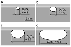
Figure 3. Illustrations of bubbles of different sizes beneath the wall in still water: (a) DB/DU ≈ 0.8, (b) DB/DU ≈ 1.6, (c) DB/DU ≈ 3.2, and (d) DB/DU ≈ 6.4.
Download figure:
Standard image High-resolution image
Figure 4. Maximum echo amplitude from bubble surface normalized with respect to that measured from the upper wall; the gray line represents the bubble surface.
Download figure:
Standard image High-resolution image2.2. Numerical simulation
2.2.1. Conditions.
We confirmed that stationary bubbles that have a relatively flat shape beneath the wall are detectable based on the echo amplitude. However, advective bubbles have different shapes to stationary bubbles and cannot be detected accurately using the same procedure. It is supposed that the maximum echo amplitude from advective bubbles is weaker as a result their round shapes. If the maximum echo amplitude from bubbles beneath the wall is similar to that from the wall, they are difficult to detect. To evaluate the extent to which the amplitude is reduced by the rounder surface, we performed numerical simulations of an ultrasonic wave reflected by a spherical bubble. We first investigated the waveform of the ultrasonic pulse emitted from the transducer for use in the simulation. To avoid noise from the UVP, the ultrasonic pulse was measured by another ultrasound transducer, which was positioned collinearly and was movable, as shown in figure 5(a). Figure 5(b) shows four sample waveforms measured at different distances from the emitter. These results demonstrate that although the ultrasonic pulse exponentially decays with distance, the waveform is maintained. The experimentally obtained waveform in figure 5(c) is modeled, and the modeled waveform is used as the emission signal in the simulation. The simulation is performed in a 3D domain, which is an authentic model of the area near the upper wall, as schematically shown in figure 6; the conditions of the domain are summarized in table 4. The finite-difference time-domain (FDTD) algorithm adopted in the present simulation is useful for solving elastic and acoustic waves at an interface [36]. In the simulation, Higdon's absorbing boundary condition is applied to prevent reflection of the ultrasonic wave at the boundaries of the calculated region [37]. It is assumed that the acoustic impedance of air (Zair) is zero, such that the ultrasonic wave is perfectly reflected at the gas/liquid interface. A 2.5 mm-diameter transducer located at the boundary of the z–x section of the elastic field emits an ultrasonic pulse with the same parameters as in the experiment and receives the echo signal. The physical properties of the acrylic resin used are representative values generally used in simulations because the properties of commercially available resins change over time and between manufacturers.
Table 4. Parameters for the numerical simulation.
| Algorithm | FDTD (finite-difference time-domain) | |
| Calculating region (Lx × Ly × Lz) | 5 × 15 × 5 | mm3 |
| Space step | 20 | μm |
| Time step | 2.5 | ns |
| Absorbing boundary condition | Higdon second order | |
| Acoustic impedance of air (Zair) | 0 | kg/m2 s |
| Speed of sound in water (cw) | 1480 | m/s |
| Density of water | 980 | kg/m3 |
| Attenuation rate in water | 0.2 | dB/m/MHz |
| Density of acrylic resin | 1190 | kg/m3 |
| Young's modulus of acrylic resin | 3.14 | GPa |
| Poisson ratio of acrylic resin | 0.35 | − |
| Attenuation rate in acrylic resin | 42 | dB/m/MHz |
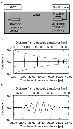
Figure 5. Ultrasonic pulse emitted from the ultrasound transducer: (a) schematic diagram of the experimental setup used to measure the pulse, (b) sample signals received at four different distances from the emitter, and (c) detailed pulse waveform.
Download figure:
Standard image High-resolution image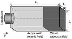
Figure 6. Schematic diagram of the 3D domain for numerical simulation of the elastic and acoustic waves, where Lx, Ly, and Lz are the distances in each direction, which are set at 5, 15, and 5 mm, respectively, contacting surface of the transducer is set on acrylic resin and located at the center of domain.
Download figure:
Standard image High-resolution image2.2.2. Echo intensity from a bubble in contact with the wall.
The two conditions shown in figure 7 (i.e. no bubble and a small spherical bubble with DB/DU = 0.8 at the liquid/solid interface) are numerically calculated, where the light gray, dark gray, and white represent acrylic resin, water, and air, respectively. Figure 8 shows the acoustic pressure of the echo averaged over the surface of the transducer (Pr) normalized with respect to the maximum acoustic pressure for ultrasonic emission (P0). In the experiment with stagnant bubbles, the maximum echo amplitude was almost 1.5 times larger than that from the liquid/solid interface (i.e. the upper wall) in the absence of bubbles. We suppose that even if a bubble has a round shape, it will produce a discriminable echo from the upper wall because the acoustic pressure is proportionally converted to a voltage by the ultrasound transducer. However, the results of the simulation indicate that the echo amplitude is almost the same with and without a bubble present. This is because the ultrasonic pulse is scattered by the round surface of the bubble, as seen in figure 9. The simulated results for bubbles of different size (DB) and oblateness (Γ) are summarized in figure 10, where PM and PW are the maximum echo amplitude with and without a bubble, respectively: Γ is defined as Γ = 1 − a/b, where a and b are the major and the minor length of the bubbles, respectively. Even for a large spherical bubble (DB/DU = 0.8 and Γ = 0) beneath the wall, PM increased by only 17% compared to the case without a bubble present because of the round bubble surface. However, for bubbles with flatter surfaces (i.e. with higher Γ), PM significantly increased. When Γ ⩾ 0.9, PM was approximately 50% higher compared to the case without a bubble present, which is in good agreement with the experimental results shown in figure 4. This means that the increased echo amplitude observed in the experiment is caused by the flatter bubble surface. To detect bubbles of the dimensions considered in the simulation based on the echo amplitude, we have to be able to detect small variations in the echo signal. For instance, the minimum increase in echo amplitude in the simulations was just 3.8% for a bubble with DB/DU = 0.6 and Γ = 0.25.

Figure 7. Conditions for the numerical simulation, where light gray, dark gray, and white represent acrylic resin, water, and air: (a) without a bubble and (b) for a small spherical bubble with DB/DU = 0.8.
Download figure:
Standard image High-resolution image
Figure 8. Echo amplitude received by the ultrasound transducer: (a) without a bubble and (b) with a small spherical bubble with DB/DU = 0.8, where signals in t ⩽ 1.00are the emission signal, the amplitude (Pr) is determined as the average of all received acoustic pressures at the surface of the transducer, P0 is the maximum acoustic pressure for ultrasonic emission, and PW and PM are the maximum echo amplitude in the absence and presence of the bubble.
Download figure:
Standard image High-resolution image
Figure 9. Ultrasonic pulse reflected from the wall: (a) without a bubble and (b) with a small spherical bubble with DB/DU = 0.8 indicated by the white circle.
Download figure:
Standard image High-resolution image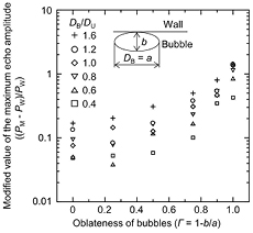
Figure 10. Ratio of the maximum echo amplitude from the surfaces of bubbles of different shapes, where the gray line indicates the maximum echo amplitude from the upper wall and DB/DU is the relative size of the bubble compared to the ultrasonic beam diameter.
Download figure:
Standard image High-resolution image2.2.3. Calculation of liquid film thickness.
Although detection of a bubble beneath the wall is possible by comparing PM with PW, this does not provide information about the thickness of the liquid film between the bubble and the wall. In cases where the liquid film thickness is measured by an ultrasonic pulse with a spatial pulse length longer than the film thickness, general measurement techniques cannot be used because the echo signals from the liquid/solid interface (i.e. the wall surface) and the gas/liquid interface (i.e. the. bubble surface) are superimposed. Therefore, to measure the liquid film thickness, it is necessary that the echo signal from the bubble is extracted from the combined signal. The black and gray lines in figure 11(a) show the waveform of the echo from the wall, W(t), and the waveform of the combined echo signal, S(t). To extract the echo waveform, S(t) is subtracted from W(t); the differential between the two signals, B(t), is shown in figure 11(b). An increase of the maximum amplitude of B(t), PB, with higher Γ is expected from the change in PM. Figure 12 shows samples of B(t) with a fixed bubble size (DB/DU = 0.6) and three different values of Γ (0, 0.5, and 1.0). An increase in Γ results not only in a higher PB as expected, but also a phase shift of the echo waveform. In the simulations, the average locations of the bubbles' upper surfaces are lifted when the bubbles have different values of Γ because they are in contact with the wall. The phase shift makes bubble detection much easier, using PB instead of PM. For example, if PM = PW and only the echo phase is shifted by the bubble, the bubble is detectable by evaluation of PB; this is not possible based on an evaluation of PM. We evaluated PB for several different bubbles in contact with the wall and the results are summarized in figure 13, where the echo from the wall is measured at PB/PW = 0. Even for a tiny bubble (DB/DU = 0.4), the calculated value of PB is more that 5% greater than PW. As previously discussed, the minimum increase in PM was 3.8%. Therefore, it is possible that bubbles near the wall are more easily detected by comparing PB and PW instead of PM and PW.

Figure 11. (a) Echo waveform without and with a bubble with DB/DU = 1.6 and Γ = 0; and (b) echo waveform from the bubble surface calculated from the two waveforms in (a).
Download figure:
Standard image High-resolution image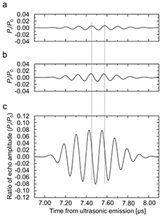
Figure 12. Changes of phase and amplitude of the echo waveforms of bubbles with DB/DU = 0.6 for different values of Γ: (a) Γ = 0.0, (b) Γ = 0.5, and (c) Γ = 1.0.
Download figure:
Standard image High-resolution image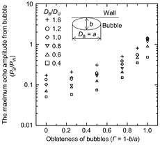
Figure 13. Maximum difference in the echo amplitudes from the upper wall and the bubble surface for different bubble oblatenesses (Γ) and relative bubble sizes (DB/DU), where PW is the maximum echo amplitude from the wall and PB = 0 means that the echo signals with and without the bubble are the same.
Download figure:
Standard image High-resolution imageB(t) provides information for measuring the liquid film thickness. When a bubble is located away from the wall, B(t) appears with a certain delay. Figure 12 shows the delayed echo waveform from a bubble located 0.2 mm from the wall. Apart from the location, the conditions of the bubble are the same as that in figure 11, which is a simulation of a bubble in contact with the wall. The echo waveform of B(t) in figure 14(b) appears with a delay of 0.27 μs relative to that in figure 11. This delay corresponds to the time required for the ultrasonic wave to complete a round trip between the wall and the bubble. Under the idealized conditions of the simulation, it is possible to accurately determine the delay and the distance. However, under experimental conditions, the accuracy of the waveform depends on the voltage resolution of the data logger. If PB is lower than the voltage resolution, the bubble is not detected. Furthermore, the properties of the wall material are unknown in many cases and it is difficult to know when an echo from the wall will appear even if the wall thickness is known. Therefore, it is necessary that the wall thickness and bubble location are determined from the echo waveforms. As seen in figure 14, the wall and the bubble can be detected when the echo amplitude exceeds a threshold. The exact distance is defined as the shortest distance between the bubble and the wall, and the distance between the wall and the bubble (dB) is calculated using the time delay (tdelay) and the speed of sound in water (cw): dB = cwtdelay/2. To evaluate the accuracy of this method, dB of six different bubbles (using three different values of DB and two different values of Γ) were investigated for four thresholds; the results are shown in figure 15. When the threshold was set at 0.2% of PM, the accuracy was within 0.1 mm although the bubble is small and spherical. Furthermore, dB increased linearly in all cases. However, the accuracy for the small spherical bubble fluctuated at large thresholds (e.g. at 5% of PM) and this bubble became undetectable when the threshold was set above PB. The resolution of the data logger used corresponds to 1.3% of PM. Although the accuracy is poor compared with that at 1.3% of PM, the linearity of dB is still maintained. From these results, it is concluded that this method is applicable for practical use if the bubbles' shapes are maintained while they traverses the ultrasonic beam.
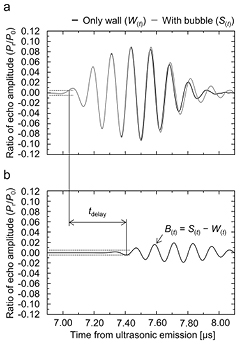
Figure 14. (a) Echo waveforms without a bubble and with a bubble with DB/DU = 1.6 and Γ = 0 that is 0.2 mm from the wall; (b) echo waveform from the bubble surface calculated from the two waveforms in (a), where the dashed lines indicate a threshold and tdelay is the delay between the two waveforms.
Download figure:
Standard image High-resolution image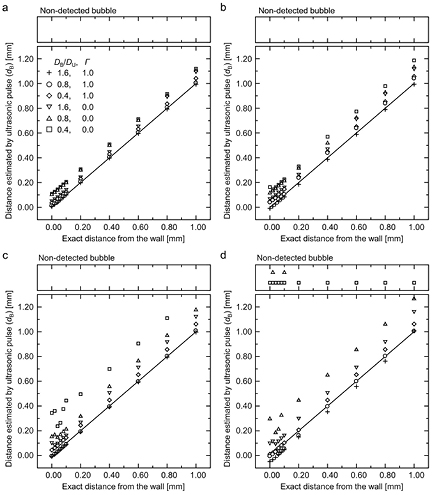
Figure 15. Accuracy of the bubble locations determined under the wall for various threshold voltages: (a) 0.2%, (b) 1.3%, (c) 5%, and (d) 10% of PM.
Download figure:
Standard image High-resolution image3. Application in real situations
3.1. Horizontal channel flow
To confirm the applicability of the present technique in real situations, the surfaces of advective bubbles were detected in a turbulent channel flow. Figure 16 is a schematic diagram of the experimental setup. The test section is a horizontal, rectangular channel composed of transparent acrylic boards, 40 mm high (2 h), 160-mm wide, 6000 mm long, and with a wall thickness of 10 mm. The x, y, and z coordinates are defined as the streamwise distance from the channel inlet, vertical distance from the upper wall, and the spanwise distance from the inner wall of the channel, respectively. Tap water at 21 °C is used as the working fluid with a kinematic viscosity (ν) of 9.8 × 10⁻⁷ m2 s−1 and speed of sound (cw) of 1486 m s−1. To generate bubbles in the test section, ambient air is injected by a compressor through an injector comprising many tiny holes mounted on the upper wall in the upstream region of the channel at x = 1.5 m. A water tank is installed at the end of the channel to remove bubbles in the flow; the water is circulated using a pump. The ultrasound transducer for echography is located on the outer surface of the upper wall, 2.0 m from the injector. The echography settings are listed in table 3; the pulse repetition frequency ( fr) was fixed at 15 kHz.

Figure 16. Schematic diagram of the horizontal channel.
Download figure:
Standard image High-resolution imageFigure 17 shows traveling bubbles beneath the wall at Reh ≈ 30 000 with αchannel ≈ 0.17%, where the Reynolds number (Reh) and void fraction (αchannel) are defined as Reh = hUbulk/ν and αchannel = Qgas/(Qliquid + Qgas); Ubulk, Qgas, and Qliquid are the bulk mean velocity of the flow, gas flow rate, and liquid flow rate, respectively. The bubble sizes in the flow are distributed in the range of 3 mm < DB < 20 mm. The echo amplitude with advective bubbles in the turbulent channel flow is shown in figure 18(a). The length scales, streamwise length (x') and depth (y) are converted from the time-domain data. The spatial resolution in each direction, Δx' and Δy, are evaluated using Taylor's hypothesis on frozen turbulence and from cw, respectively: Δx' = uB/fr and Δy = cw/2fs, where the average value of uB is obtained using a camera. A large echo amplitude exists under the upper wall and an echo signal modified by the surfaces of the bubbles also appears. The modified echo signal nearest to the top wall at each value of x' is plotted in figure 18(b). These plots represent the upper surfaces of the bubbles. There sizes of the two bubbles in figure 18 were measured from the camera images. The bubbles have a flat upper surface because of the upper wall and their buoyancy. Moreover, the top of each bubble experiences a lift force because bubbles have higher advection velocities than the streamwise velocity of the ambient water flow near the wall and move to a downstream region. Depending on their shape and the lift force, the advective bubbles may have a liquid film above them. This shape-dependent behavior was previously studied by optical visualization and the results are shown in figure 19 [38]. In summary, we have demonstrated the successful application of this bubble detection system with high temporal resolution.
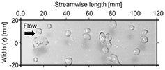
Figure 17. Snapshot picture of advective bubbles in the channel flow taken from above in the test section.
Download figure:
Standard image High-resolution image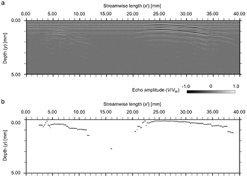
Figure 18. Advective bubbles in a turbulent channel flow with Reh = 30 000: (a) original echo amplitude distribution and (b) detected upper surfaces of bubbles.
Download figure:
Standard image High-resolution image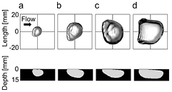
Figure 19. Shapes of bubbles in a channel flow with Reh = 18 520 obtained by optical visualization: (a) DB ≈ 10 mm, (b) DB ≈ 20 mm, (c) DB ≈ 26 mm, and (d) DB ≈ 28 mm, where the upper and lower panels are the top and side views, respectively. Figure taken with permission from Oishi and Murai (2014) [38], courtesy of Y Murai.
Download figure:
Standard image High-resolution image3.2. Model ship experiment
Experiments using a model ship were designed to evaluate the ultrasonic bubble measurement system. The experiments were performed in a towing tank at Hiroshima University. The experimental parameters are listed in table 5. The water temperature in the tank was 24 °C and the viscosity and speed of sound were ν = 9.2 × 10⁻⁷ m2 s−1 and c = 1494 m s−1, respectively. A photograph and schematic diagrams of the model ship are shown in figure 20. The model ship was made of transparent acrylic resin with dimensions of 4000 mm in overall length (L), 600 mm in width (W) and 500 mm in height (H). The x, y, and z coordinates are defined as the streamwise distance from the leading edge, vertical position from the bottom plate, and spanwise position from the center of the ship, respectively. To avoid the effects of the wave generated by the prow, two side walls were installed at y = 20 mm, as shown in figure 20(d). To simulate a boundary layer on a flat plate, the ship bottom was constructed using a flat plate, and the leading edges of the bottom plate and two side walls were machined at 45°. Bubbles were injected by an air injector located at x = 0.7 m. Air was introduced to a buffer chamber with a total volume of 5.0 × 10⁻³ m3 by a compressor, and injected into the boundary layer through a 100 μm-diameter porous plate, as shown in figure 20(e). An ultrasound transducer for bubble detection was placed on the upper surface of the bottom wall at x = 2.2 m. The echography settings are listed in table 3; fr was fixed at 20 kHz.
Table 5. Parameters of the model ship experiment.
| Towing tank | ||
| Length | 80 | m |
| Depth | 3.5 | m |
| Width | 8 | m |
| Towing train | ||
| Acceleration | ±0.1 | m/s2 |
| Maximum speed | 3.00 | m/s |
| Model ship | ||
| Material | acrylic resin | |
| Length (L) | 4000 | mm |
| Height (H) | 500 | mm |
| Width (W ) | 600 | mm |
| Weight (empty load) | 149.2 | kg |
| Draft (empty load) | 68 | mm |
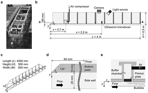
Figure 20. (a) Overview photograph of the ship. (b–e) Schematic diagrams of the side view of the ship, overview of the ship, leading edge, and injector, respectively.
Download figure:
Standard image High-resolution imageFigure 21 is a snapshot picture of bubbles traveling beneath the ship bottom taken by a camera located above the ultrasound transducer at a towing speed (Uship) of 2.0 m s−1 and Qgas of 100 L min−1. The Reynolds number on the flat plate (Rex) without bubbles and the void fraction on the boundary layer estimated from its thickness (αδ) are 4.8 × 10⁶ and 4.2%, respectively. They are defined as Rex = xUmain/ν and αδ = Qgas/(Qliquid + Qgas) ≈ Qgas/W where the 99% turbulent boundary layer thickness (δx) and streamwise velocity distribution (uy) in the layer are assumed as δx = 0.37x/
 and uy = Umain(y/δx)1/7, respectively. Bubbles with a broad size distribution (DB ≈ 1–20 mm) have the interfacial wave as indicated by the shadows on their upper surfaces in the figure. Capillary waves on the bubbles' surfaces indicate that a liquid film exists between the wall and the bubbles. Although the visualization confirms the presence of the liquid film, it cannot be used to estimate its thickness. Figure 22(a) shows an original echo distribution under the bottom of the ship used to measure the film thickness. The echo distribution is modified when bubbles pass under the ultrasound transducer. The upper surfaces of the bubbles detected using the modified echo are shown in figure 22(b). The thickness of the liquid film is determined to be approximately 0.1–1 mm from the gas/liquid interface.

Figure 21. Snapshot picture of bubbles traveling beneath the bottom of the ship taken by a camera placed above the ultrasound transducer.
Download figure:
Standard image High-resolution image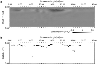
Figure 22. Result of the ultrasonic measurement performed on the model ship: (a) original echo amplitude distribution and (b) detected upper surfaces of bubbles.
Download figure:
Standard image High-resolution image
4. Conclusions
Heat, mass, and momentum transfer in a turbulent boundary layer in the vicinity of a wall are affected by the behavior of bubbles in the layer. In particular, the thickness of the liquid film between the wall and the traveling bubbles is important. We designed an ultrasonic echography system that can be applied under the typical flow conditions of ships. A relatively long spatial pulse length (0.76 mm) was used to ensure deep propagation of the pulse and to allow it to be coupled with ultrasonic velocity profiling (UVP). Bubbles larger than 1 mm were easily detected with the present echography system because they migrate at speeds between 0 and 37 m s−1. The measurable range depends on the diameter of the ultrasonic beam and the pulse repetition rate as long as the signal-to-noise ratio of the echo intensity is kept high. 3D numerical analysis of the wave equation for bubbles of different sizes and shapes, and at different locations confirmed that the measurement principle is valid if the echo waveform from the wall in the absence of bubbles is determined. The best spatial resolution of the bubble surface was 0.5λ (where λ is the fundamental ultrasonic frequency) and the poorest resolution was 1.5λ for spherical bubbles smaller than the diameter of the ultrasonic beam. After optimization of the experimental parameters, the technique was applied for bubble monitoring for two different experimental configurations: a horizontal channel and a model ship subjected to bubbly turbulent flow in the boundary layer. In both configurations, the streamwise length of bubbles and the shape of the bubbles' upper surfaces, obtained from liquid film thickness located on the ultrasound beam, agreed quantitatively with optical visualizations. Furthermore, bubbles accompanying liquid films that fluctuate rapidly were successfully measured although their characteristic thickness was approximately 0.1–1.0 mm (i.e. shorter than λ). Various extensions of this technique may follow in the future. For example, the ultrasound transducers may be positioned at different locations in spanwise and streamwise directions, which would result in spanwise bubble oblateness and improve the migration velocity, respectively.
Acknowledgments
This work was supported by the Fundamental Research Developing Association for Shipbuilding and Offshore (REDAS), Grant-in-Aid for JSPS Fellows No. 15J00147, JSPS KAKENHI Grant Nos. 24246033 and 23760143. The authors would like to express their appreciation for this support.