

Abstract
The flatness of an optical surface can be evaluated using a Fizeau interferometer. There is strong demand for ensuring that the measurement uncertainty of flatness is of nanometer order over a measurement range of 300 mm or more; however, the measurement range and measurement uncertainty of flatness at the National Metrology Institute of Japan (NMIJ) are 300 mm and 10 nm, respectively. In a Fizeau flatness interferometer, the gap distance between the reference flat and the specimen is measured. To obtain the absolute profile of the specimen, the absolute profile of the reference flat should be measured in advance. The three-flat test is one of the methods used to measure the absolute profile of a reference flat. The reference flat, however, deforms under the force of gravity, and its absolute deformation value cannot be determined by the three-flat test. The deformation value of the reference flat can be corrected by the finite element method (FEM) analysis; however, it is difficult to ensure the validity of the analysis and there is a large uncertainty component of the Fizeau flatness interferometer. To verify the FEM analysis, we developed a scanning deflectometric profiler (SDP) that does not require a reference flat and can directly measure a profile. We calibrated an optical flat using a Fizeau flatness interferometer and the SDP. Finally, the deformation value of the reference flat under the force of gravity was evaluated by comparing the measurement results.
Export citation and abstract BibTeX RIS
1. Introduction
There is strong demand for ensuring that the measurement uncertainty of flatness is of nanometer order over a measurement range of 300 mm or more. At the National Metrology Institute of Japan (NMIJ), we have a large-aperture high-precision Fizeau flatness interferometer (see figure 1). Its measurement range and measurement uncertainty of flatness are 300 mm and 10 nm (k = 2), respectively.
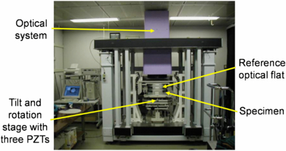
Figure 1. Large-aperture Fizeau flatness interferometer.
Download figure:
Standard image High-resolution imageIn the Fizeau flatness interferometer, the gap distance between a reference flat and a specimen is measured. To obtain the absolute profile of the specimen, the absolute profile of the reference flat should be measured in advance. The three-flat test is one of the methods used to measure the absolute profile of a reference flat [1–7]. In the three-flat test, three almost identical flats are prepared, and all combinations of two flats selected from three are compared. Solving three simultaneous equations (i.e. three measurements) for three unknown variables (i.e. three flats) yields the absolute profile of the flats. The three-flat test is a self-calibration technique; however, it has a problem. Figure 2 shows the situation of one combination measurement of the three-flat test. Figures 2(a) and (b) are no gravity condition and under gravity condition, respectively. Assuming that both optical flats have no profile error, the interferometer result is the flat-profile in no gravity condition. In actuality, both optical flats bend under the gravity condition. On the other hand, the deformation value of both optical flats is same. The same measurement results in both conditions are obtained. This is the problem that the absolute deformation value of the reference flat cannot be determined by the three-flat test. The deformation value of the reference flat can be corrected by finite element method (FEM) analysis; however, it is difficult to ensure the validity of the analysis and there is a large uncertainty component of the Fizeau flatness interferometer.
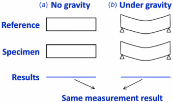
Figure 2. Effect of deformation under force of gravity.
Download figure:
Standard image High-resolution imageThus, we developed a scanning deflectometric profiler (SDP) that does not require a reference flat and can directly measure a surface profile. Various deflectometric systems have been developed for measuring a highly accurate optical surface profile [8–16]. In this study, we measured an optical flat using a Fizeau flatness interferometer and the SDP. It was verified that the deformation value for the reference flat under the force of gravity could be corrected by comparing the measurement results.
2. Problem of Fizeau flatness interferometer
2.1. Deformation of reference flat under gravity
Figures 3 and 4 respectively show a photograph and a cross-sectional view of the reference flat. The reference flat is 350 mm in diameter and 100 mm in thickness, and is made of synthetic fused silica. It is mounted in an aluminum ring with 54 supporting points as shown in figure 4. The deformation value of the reference flat under the force of gravity was calculated by FEM analysis [17]. The deformation value of the reference flat was 23 nm in the case of a 300 mm diameter. A correction map of the reference flat was made from the results of the three-flat test and FEM analysis.

Figure 3. Photograph of the reference flat.
Download figure:
Standard image High-resolution image
Figure 4. Cross-sectional view of the reference flat.
Download figure:
Standard image High-resolution image2.2. Validation of deformation analysis
To verify the FEM analysis results, the deformation value of the reference flat was experimentally measured. Figure 5 shows a schematic view of the experimental measurement. First, the surface profile of the reference flat is measured with respect to another optical flat before the reference flat is mounted in the aluminum ring. Then, the same measurement is carried out after the reference flat is mounted. Finally, the difference between the two results gives the deformation value of the reference flat under the force of gravity.

Figure 5. Systematic view of the experimental measurement to obtain the deformation value of the reference flat under the force of gravity.
Download figure:
Standard image High-resolution imageFigure 6 shows a comparison of the results by FEM analysis (solid line) and experimental measurement (dotted line). The conditions of the FEM analysis and experimental measurement are reported in detail in the literature [17]. The results show good agreement, but there is a peak-to-valley (P–V) difference of a few nanometers. The difference between experimental and calculated results is a major source of uncertainty of the Fizeau flatness interferometer. To reduce the uncertainty of the Fizeau flatness interferometer, it is necessary to improve the evaluation of the reference flat under the force of gravity.
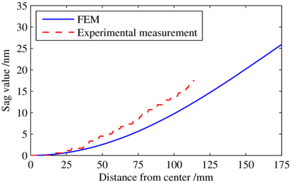
Figure 6. Comparison of results obtained by the FEM analysis and experimental measurement.
Download figure:
Standard image High-resolution image3. Development of scanning deflectometric profiler
3.1. Principle of SDP
We developed the SDP to evaluate the deformation value of the reference flat. The SDP does not require a reference flat and can directly measure the surface profile.
Figures 7 and 8 show a schematic view and a photograph of the developed SDP, respectively. The SDP is constructed using an autocollimator and a pentamirror fixed on an air slide table. The travel distance of the air slide table is 1.2 m. The measurement beam of the autocollimator is bent by the pentamirror so that it illuminates a specimen. The optical system of the SDP is aligned according to the literature [18–20] of an alignment procedure for a deflectometry system. The size of the measurement beam is  34 mm. An aperture is set in front of the specimen for increasing the special frequency. Local slope angles at each position of the specimen are measured by scanning the pentamirror. The pentamirror is effective for minimizing the moving error during scanning, and the influence of the moving error on the local slope angle measurement is negligible [18–20]. The surface profile F(xi) of the specimen is obtained by integrating the local slope angles as follows:

where i is a measurement number, N is the total number of measurement points, f(xi) is a profile, f'(xi) is a measured local slope angle and xi is measurement position. The measured slope angle f(x1) of the first measurement position x1 can be selected as an arbitrary angle. The numerical integration of equations (1) and (2) is calculated such that the measured angle of the first measurement position is zero. A dc component a0 of the measured slope angle f'(xi) is a line g(xi) = a0xi + b. Then, the least-squares line g(xi) is calculated from the profile f(xi). By subtracting g(xi) from f(xi), we can obtain the final profile F(xi) as follows:


Figure 7. Schematic view of the SDP.
Download figure:
Standard image High-resolution image
Figure 8. Photograph of the SDP.
Download figure:
Standard image High-resolution image3.2. Measurement accuracy
We used a commercial autocollimator (MÖLLER-WEDEL OPTICAL GmbH, ELCOMAT 3000) of which the total measurement range and the resolution are ±1000 arcsec (5.1 mrad) and 0.001 arcsec (4.8 nrad), respectively. The measurement accuracy of the autocollimator is the most important aspect of the SDP based on the angle measurement. We calibrated the autocollimator using a high-accuracy angle index table at NMIJ. The index table is controlled in arbitrary angle positions around 360° using a rotary encoder of which the total number of graduation lines and the electric interpolator are 225 000 and 2048 times division, respectively; therefore, the index angle resolution is 0.0028 arcsec (13.6 nrad). The servo-control stability is about ±1 pulse (±0.0028 arcsec). Figure 9 shows a photograph of a calibration setup of the autocollimator. We set a highly reflective mirror on the index table. The distance between the autocollimator and the mirror is 160 mm. The autocollimator is calibrated by measuring the rotation angle of the mirror. NMIJ is making an uncertainty budget for measuring a rotation angle, though the measurement accuracy is less than 0.005 arcsec. The measurement system of a rotation angle is reported in detail in the literature [21]. The evaluation results of the autocollimator using the high index table are described in the following sections.

Figure 9. Photograph of the high-accuracy angle index table.
Download figure:
Standard image High-resolution image3.2.1. Random error
Figure 10 shows the short-term stability of the autocollimator, when the mirror is controlled at an angular position. The sampling rate and the number of measurement points were 25 Hz and 100 points, respectively. The standard deviation σrand was 0.008 arcsec (38.9 nrad).
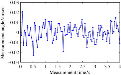
Figure 10. Stability of the autocollimator.
Download figure:
Standard image High-resolution imageAs a surface profile is calculated by integrating the local slope angles at each measurement position, the random error is also integrated. The standard uncertainty urand of the random error is given by

where N and dx are the total number of measurement points and the scanning pitch, respectively. When N and dx are 300 points and 1 mm, respectively, the standard uncertainty is 0.67 nm. The final profile F(xi) is obtained by subtracting a dc component of the measured angle slope f'(xi) from equation (3); therefore, a dc component of an integrated random error is also subtracted. Equation (4) is overestimated but the expected value of the random error is zero and the overestimated value is very small.
3.2.2. Systematic error
The reference flat of the Fizeau flatness interferometer is approximated by the quadratic curve of the concave surface. The maximum profile deviation (sag value) and the maximum deviation of the local slope angle over the measurement range of 300 mm are 23 nm and ±0.06 arcsec, respectively. Thus, the measurement range of the autocollimator is very small. Figure 11 shows the calibration curve of the autocollimator. The range and pitch of the calibration angle were ±5 arcsec and 0.05 arcsec, respectively. The maximum deviation ea of the angle over the range of calibration (P–V value) was 0.032 arcsec (155.1 nrad). The measurement range of the autocollimator varies with the surface profile of the specimen. We assume that the standard deviation of the systematic error is set to be the uniform distribution of the maximum angle deviation of the calibration curve, then the standard uncertainty usys of the systematic error is given by

N and dx are 300 points and 1 mm, respectively, and the standard uncertainty is 0.78 nm.
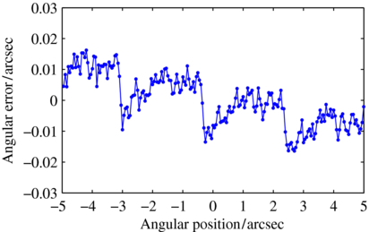
Figure 11. Calibration curve of the autocollimator.
Download figure:
Standard image High-resolution imageThe literature [11, 22–24] reported that the systematic error of an autocollimator is changed by measurement conditions: distance between an autocollimator and a mirror, aperture size and reflectance. The evaluation results in figures 10 and 11 were only one condition. We are estimating an uncertainty budget of the SDP from a number of measurement conditions.
4. Comparison measurement between a Fizeau flatness interferometer and an SDP
4.1. Comparison method
To verify the FEM analysis results, we measured an optical flat using the Fizeau flatness interferometer and the SDP. Figure 12 shows a photograph of the optical flat used for comparison, which is 340 mm in diameter and 70 mm in thickness, and is made of the ultralow-expansion ceramic NEXCERA™. A mask of size 300 mm × 30 mm is placed on the optical flat. The comparison measurement is performed along the center line of the mask.
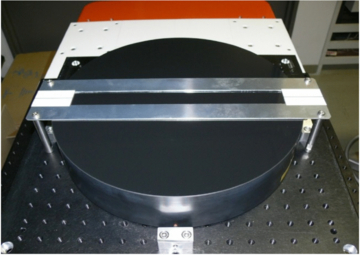
Figure 12. Photograph of the optical flat used for comparison.
Download figure:
Standard image High-resolution image4.2. Fizeau flatness interferometer
The optical flat was set up on the rotary stage of the Fizeau flatness interferometer. The flatness of the optical flat within the mask area was measured. After the measurement, the optical flat was rotated 30°. Then, the flatness measurement was performed again. As a result, the optical flat was set up in 12 different orientations and measured in each orientation. Figure 13 shows the measurement results for each orientation. The orthogonal coordinate XY is the CCD camera coordinate of the Fizeau flatness interferometer and all orientation results have a common coordinate. The pixel size is 1024 × 1024 and the lateral size is about 0.34 mm/pixel. Figure 14 shows the center line of the mask, which was extracted from the measurement results for each orientation. The P–V value and the root mean square (RMS) value for the average curve of the measured profiles were 32.7 nm and 10.8 nm, respectively. The standard deviation of the P–V value and the RMS value for each orientation were 0.46 nm and 0.11 nm, respectively. Figure 15 shows the difference curves from the average center line curve for each orientation. The profiles for each orientation are in good agreement, and the dispersion excluding the spike noise was about ±1 nm. This result indicates the reliability of the correction map for the reference flat of the Fizeau flatness interferometer obtained by the three-flat test. However, this result does not validate the correction map for the deformation under the force of gravity obtained by FEM analysis. This is because of the axisymmetrically deformed profile. The correction map for the deformation is an axisymmetrical profile. When a profile of an optical flat with respect to a different line of the reference flat is measured, the amount of correction for a deformation of the reference flat is not changed. Thus, the correction map for the absolute deformation value of the reference flat cannot be validated from the results in figures 13–15.

Figure 13. Measurement results of the optical flat obtained by using a Fizeau flatness interferometer.
Download figure:
Standard image High-resolution image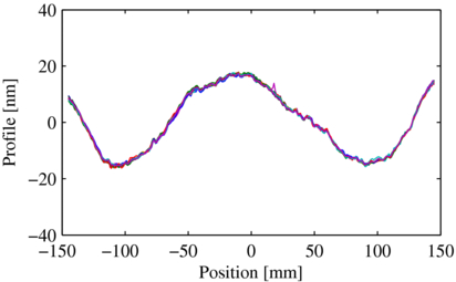
Figure 14. Center line of mask for 12 measurement orientations.
Download figure:
Standard image High-resolution image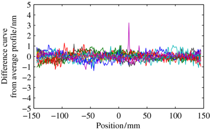
Figure 15. Dispersion of center line measurement from each orientation.
Download figure:
Standard image High-resolution image4.3. Scanning deflectometric profiler
The profile of the optical flat was measured using the SDP. The aperture size was  8 mm and the scanning pitch was 1 mm. To avoid drift, we adopted a measurement strategy [25] in which the measurement was performed in four directions: forward, backward, backward and forward. Figure 16 shows the measured local slope angle. The measurement range of the autocollimator was about 0.4 arcsec. The profile was calculated by integrating the curve obtained by averaging the four obtained measurement curves. Figure 17 shows the calculated profile. There are 10 profiles, that is, the total number of measurements was 40. The P–V value and the RMS value for the average curve of the measured profiles were 32.2 nm and 10.5 nm, respectively. The standard deviation of the P–V value and the RMS value for ten profiles were 0.62 nm and 0.15 nm, respectively. Figure 18 shows the difference curves from the average profile curve. The repeatability was ±1.3 nm.

Figure 16. Measured local slope angle.
Download figure:
Standard image High-resolution image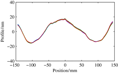
Figure 17. Profile measured using the SDP.
Download figure:
Standard image High-resolution image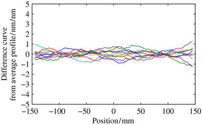
Figure 18. Repeatability of profile measurement.
Download figure:
Standard image High-resolution image4.4. Difference between Fizeau flatness interferometer and SDP
Figure 19 shows the measurement results obtained by the two different methods. The P–V values for the Fizeau flatness interferometer and SDP were 32.7 nm and 32.2 nm, respectively. The RMS values for the Fizeau flatness interferometer and SDP were 10.8 nm and 10.5 nm, respectively. Figure 20 shows the difference curve between the Fizeau flatness interferometer and the SDP. The measurement results are in good agreement, and the P–V value and the RMS value for the difference curve were 3.3 nm and 0.60 nm, respectively. For the Fizeau flatness interferometer, when the correction map for the deformation value of the reference flat under the force of gravity calculated by the FEM analysis is incorrect, the difference curve has a quadratic component. As a result, the quadratic component of the difference curve was less than 1 nm P–V. The comparison results validate the correction map for the reference flat obtained using the Fizeau flatness interferometer by the three-flat test and FEM analysis.
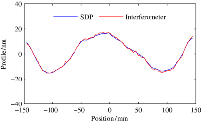
Figure 19. Measurement result based on two different methods.
Download figure:
Standard image High-resolution image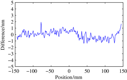
Figure 20. Comparison of results between the interferometer and the SDP.
Download figure:
Standard image High-resolution image
5. Conclusions
In a Fizeau flatness interferometer, the correction of the reference flat is important. The three-flat test could be used to measure the profile of the reference flat; however, the deformation value under the force of gravity cannot be determined, although its deformation value can be calculated by finite element method (FEM) analysis. To verify the FEM analysis, we developed a scanning deflectometric profiler (SDP) that does not require a reference flat and can directly measure a surface profile. In this study, we performed a comparison measurement between a Fizeau flatness interferometer and the SDP. Then, the correction map of the reference flat obtained by the three-flat test and FEM analysis was verified. To reduce the uncertainty of the Fizeau flatness interferometer, the next task is to estimate the uncertainty of the developed SDP.