

Abstract
A novel method is presented to quantify the uncertainty of PIV data. The approach is a posteriori, i.e. the unknown actual error of the measured velocity field is estimated using the velocity field itself as input along with the original images. The principle of the method relies on the concept of super-resolution: the image pair is matched according to the cross-correlation analysis and the residual distance between matched particle image pairs (particle disparity vector) due to incomplete match between the two exposures is measured. The ensemble of disparity vectors within the interrogation window is analyzed statistically. The dispersion of the disparity vector returns the estimate of the random error, whereas the mean value of the disparity indicates the occurrence of a systematic error. The validity of the working principle is first demonstrated via Monte Carlo simulations. Two different interrogation algorithms are considered, namely the cross-correlation with discrete window offset and the multi-pass with window deformation. In the simulated recordings, the effects of particle image displacement, its gradient, out-of-plane motion, seeding density and particle image diameter are considered. In all cases good agreement is retrieved, indicating that the error estimator is able to follow the trend of the actual error with satisfactory precision. Experiments where time-resolved PIV data are available are used to prove the concept under realistic measurement conditions. In this case the 'exact' velocity field is unknown; however a high accuracy estimate is obtained with an advanced interrogation algorithm that exploits the redundant information of highly temporally oversampled data (pyramid correlation, Sciacchitano et al (2012 Exp. Fluids 53 1087–105)). The image-matching estimator returns the instantaneous distribution of the estimated velocity measurement error. The spatial distribution compares very well with that of the actual error with maxima in the highly sheared regions and in the 3D turbulent regions. The high level of correlation between the estimated error and the actual error indicates that this new approach can be utilized to directly infer the measurement uncertainty from PIV data. A procedure is shown where the results of the error estimation are employed to minimize the measurement uncertainty by selecting the optimal interrogation window size.
Export citation and abstract BibTeX RIS
1. Introduction
Digital particle image velocimetry (PIV) is nowadays an established and reliable flow diagnostic tool capable of measuring velocity fields in two- and three-dimensional (3D) domains. Several works have been focused on PIV measurement errors. Fincham and Spedding (1997) distinguished two major forms of errors in digital PIV, namely the mean-bias error and the root-mean-square (RMS) error of the remaining fluctuations (or random error). The bias error arises from the inadequacy of the statistical method of cross-correlation in the evaluation of PIV recordings. A bias error of the measured displacement toward the closest integer value occurs when the particle image size is small with respect to the pixel size; this effect is commonly referred to as peak-locking and is responsible for measurement errors up to 0.1 pixels (Westerweel (1997), Scarano and Riethmuller (2000) among others). A bias error that underestimates the amplitude of a velocity spatial fluctuation within the interrogation window (modulation error) arises from the spatial filtering effects when the length scale of spatial fluctuations is equal to or smaller than the interrogation window (Nogueira et al 2005, Scarano 2003, Schrijer and Scarano 2008). Despite the attention devoted to the properties of bias errors in PIV, the random component most often dominates the measurement error. A first estimate of the measurement error is based on evaluating the width of the particle images (Adrian 1991). It is theoretically demonstrated that the autocorrelation peak width is proportional to the particle image diameter. A simple predictive model is that the error is directly proportional to the correlation peak width. However, many more parameters play a role for random-type errors. The change of relative intensity between particle images at first and second exposure was demonstrated to be the source of large errors (Nobach and Bodenschatz 2009). This occurs in the presence of out-of-plane particle motion or when the two laser sheets are not well overlapping. Also fluctuating background intensity and camera noise introduced during the recording process contribute to increase the amplitude of random errors. Several studies have indicated typical values for the random errors. Westerweel (2000) reported a typical figure of 0.05 pixels from Monte Carlo simulations. Very similar values were obtained by Raffel et al (1998). The random error is also reported to be highly sensitive to the interrogation procedure; for instance Scarano and Riethmuller (2000) measured an RMS error three times smaller when comparing iterative window deformation to the discrete window shift technique (Westerweel et al 1997). The use of window weighting functions and of advanced interpolators is also shown to affect the amplitude of the random error (Astarita 2007).
A special case of PIV error is introduced by false correlation peak detection. This mostly occurs when the correlating windows produce an insufficient number of particle image pairs, for instance due to low seeding density or out-of-plane motion. The result is the occurrence of spurious vectors (Huang et al 1997). The error associated with a spurious vector is typically orders of magnitude larger than the typical random error. Recognizing and eliminating such incorrect vectors is a mandatory step to obtain unbiased velocity statistics and the procedure is referred to as data validation (Westerweel 1994, Westerweel and Scarano 2005).
As should be clear from the above, efforts to estimate the error of PIV measurements have mostly followed a priori approaches based on modeling the measurement chain, from the tracer motion and imaging to the digital image analysis (Westerweel 1997). In most cases the results are obtained with Monte Carlo simulations. Theoretical models have been formulated to evaluate the effects of several measurement conditions (velocity gradient, particle image diameter and image intensity, among others) on the measurement precision (Westerweel 2000, 2008). However, some results are valid only for simple interrogation methods (discrete window shift, Westerweel et al (1997)). In contrast, state-of-the-art methods, such as iterative window deformation, are less prone to some of the errors (Fincham and Delerce 2000, Scarano and Riethmuller 2000), but their theoretical modeling is more complex. Finally, the Monte Carlo approach reaches its limits when more realistic measurement conditions are to be numerically modeled and simulated. It is generally accepted that computer-based simulations lead to a significant underestimation of the measurement error due to the adoption of too idealized conditions (Megerle et al 2002, Stanislas et al 2008). Nevertheless, to date, very realistic simulations of turbulent flow measurements have been achieved in the study of Lecordier et al (2001).
Despite the above efforts, the a priori estimate of the measurement error based on numerical simulations or on simplified models cannot account for the many parameters that affect the measurement precision. As a result, the investigator is too often left with the empirical universal constant of 0.1 pixels as a typical figure for measurement error. A popular strategy is also to vary a few parameters and try to optimize the result with respect to the perceived error level. The most common exercise is that of gradually varying the interrogation window size. At any reduction step, the nominal measurement spatial resolution increases at the cost of an increase of the measurement noise. When the noisy fluctuations exceed the level considered acceptable, the measurement is regarded as noise-dominated and a slightly larger interrogation window is selected as optimal for data analysis. Clearly, such a procedure is largely dependent upon human perception of the signal quality and the embedded noise and cannot be proposed as a rigorous approach to error estimation.
The above case is a crude first example of a posteriori PIV data analysis and error estimation. The objective of this work is to establish the founding principles of an a posteriori error estimation technique, aiming at quantitative and objective evaluation of the measurement error and its statistics. Currently, the topic of PIV error and uncertainty estimation is frequently addressed and recognized as very important in the experimental fluid mechanics community, where PIV plays a prime role as diagnostic tool. The issue is of particular importance when PIV is used to assess the validity of results obtained with computational fluid dynamics. The 'PIV uncertainty workshop' held in Las Vegas in 2011 is only one of the events that demonstrates such attention. Only in a recent work, Timmins et al (2012) introduced a method for the automatic uncertainty estimation of PIV measurements. The approach consists in identifying the main error sources and determining their contribution to the measurement error via Monte Carlo simulation. The method can be categorized as a posteriori because it makes use of information taken from the measurement conditions (particle image diameter, particle density, particle displacement and velocity gradient). The measurement uncertainty is retrieved from numerical simulations conducted under the measurement conditions encountered in the experiment. As already stated, the amplitude of the errors returned from the numerical simulations is often significantly lower than the actual experimental error. Furthermore, the uncertainty computed with this method is typically underestimated because only a limited number of error sources is taken into account.
Charonko and Vlachos (2013) proposed an a posteriori uncertainty quantification based on the cross-correlation peak ratio. The method has been shown to be effective for the robust phase correlation (Eckstein and Vlachos 2009), while it yields unreliable uncertainty prediction for the standard cross-correlation technique.
Other methods that have followed a posteriori error estimation are based on the application of governing laws to the measured velocity field. In 3D data from incompressible flows, the fluctuating velocity divergence (Liu and Katz 2006, Scarano and Poelma 2009) indicates the error level of the velocity and its derivatives. Unfortunately, in planar experiments of turbulent flows, mass conservation cannot be imposed due to the 3D flow motion.
This work describes a method for quantifying the uncertainty of PIV measurements. The work focuses on the errors arising from the vector computation and puts most attention on the random error. However, also the systematic error due to spatial modulation can be detected by the present approach. Instead, errors arising from spurious vectors, those due to temporal modulation (truncation errors) and to other aspects of the measurement chain (such as timing errors, perspective errors, magnification errors, calibration errors, etc), are not given attention in the present framework. The proposed approach is based on the concept of super-resolution (Keane et al 1995, Cowen and Monismith 1997), in the sense that the contribution of individual particle images to the correlation peak is considered to infer the measurement standard uncertainty, which is the estimation  of the unknown actual error δ. The expanded uncertainty estimate
  is finally defined as the interval about the measurement which contains the measurand at a confidence level that depends on the chosen k.
2. Working principle of the image-matching uncertainty quantification
2.1. The method in brief
It is assumed here that the PIV interrogation process is performed by means of spatial cross-correlation of a pair of images. The analysis of the correlation map yields the position of the peak with sub-pixel precision obtained by 3-point Gaussian fit (Willert and Gharib 1991). The result is the instantaneous velocity field V = (u, v) at discrete positions x corresponding to the center of each interrogation window. By this method, the only information somehow related to the measurement uncertainty is given by the correlation signal-to-noise ratio, usually defined as the ratio between the highest peak and the second highest peak.
In this discussion we consider three possible interrogation methods with increasing level of complexity:
- (1)single-pass correlation (Keane and Adrian 1992);
- (2)double-step analysis with discrete window offset (Westerweel et al 1997);
- (3)
For simplicity, we will explain the working principle considering the second method. However, the proposed methodology is generally applicable to these three methods and other ones, if based on cross-correlation analysis.
Let us consider two exposures of a set of particle tracers in motion. Applying the cross-correlation analysis, the mean particle image displacement is obtained, which is denoted as Δx here. Now, if the window from the second exposure is shifted toward the first exposure with the closest integer approximation (see Westerweel et al (1997) for details), most particle images will come to partly superimpose. However, a number of particle pairs will not correspond exactly. This can be caused by several factors: first, the particle image displacement is generally different from an integer number of pixels; second, particles may displace by different amounts due to the velocity gradient; particle images may partly or totally disappear due to the out-of-plane particle motion (figure 1, particle image number 4). Furthermore, a randomly distributed disparity vector with fractional pixel amplitude will also occur due to the presence of noise in the recordings.
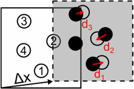
Figure 1. Particle image disparity after the discrete window offset.
Download figure:
Standard imageWith the discrete window offset technique, the shift between windows is approximated to the closest integer number of pixels. Therefore the particle pairs will generally mismatch by a constant value not larger than half a pixel.
The residual distance d between the pair of particle images after the matching is called here matched particle image disparity. The basis of the present method is the statistical analysis of such disparity, which returns the estimate for the velocity vector measurement error.
2.2. Detailed implementation
The main elements composing the principle of the proposed approach are four.
- (a)Image matching: the particle pairs are matched at the best of the velocity estimator.
- (b)Particle image pair detection: particle images occurring in both exposures and falling close to each other are detected as a pair.
- (c)Disparity vector computation: the distance between the particle image pair is evaluated as the distance between their centroids.
- (d)Statistical analysis of disparity vector ensemble: the mean value and the statistical dispersion of the disparity vectors of particle pairs belonging to the interrogation window are used to estimate the velocity vector error.
Since the measurement error is estimated via a statistical analysis of the disparity vector ensemble, the accuracy of the method depends on the particle image density. It can be proven that the variance of the uncertainty estimate is inversely proportional to the number N of particle images within the interrogation window. A minimum number of about six particle images per interrogation window is required for accurate error estimation.
2.2.1. Image matching
Let us consider a pair of images I1 and I2 separated by a time interval Δt. We refer here to the interrogation technique based on spatial cross-correlation that determines the group velocity of the particles inside a chosen window.
The procedure of image matching is based on the principle that one image is taken as reference pattern and the second one is subject to a transformation that minimizes the distance (typically L2-norm) between the two images. The match between the two images is based on an estimate of the velocity field (velocity predictor). This is commonly performed by multi-step interrogation, either with window shift or by deformation.
The degree of matching will depend on many parameters: the size of the interrogation window, the flow length-scales, the out-of-plane motion and the algorithm used. The method based on discrete offset will match the particle motion within uniform (planar) velocity approximation; the image deformation method will match the particle motion up to a piecewise linear approximation (Scarano 2002, Astarita and Cardone 2005). The matched images are indicated with  and
and  , respectively.
It is important to remark that in the matched images the particle images should superimpose to a large degree. To explain the working principle of the technique, the distinction between the ideal case (perfect particle images with only planar motion and no noise) and real case is remarked hereafter. In the ideal case, the particle images of a pair superimpose perfectly in the matched images  and
and  ; therefore, the cross-correlation function exhibits a displacement peak centered at the origin (null relative displacement) or at the fractional displacement (equal for all the particle images within the window) with a peak width proportional to the particle image diameter dτ, as illustrated in the first row of figure 2. As discussed by Adrian (1991), the uncertainty of the displacement measurement is also proportional to the particle image diameter dτ. Later studies have also discussed the dependence upon the interrogation algorithm employed to locate the particle centroid (Lourenço and Krothapalli 1995).
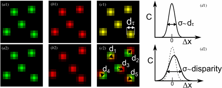
Figure 2. First row: image matching in the ideal case. (a1) Particle images of  ; (b1) particle images of
  ; (c1) superposition of
  and
and  : the green particles of
  and the red particles of
  superimpose perfectly, yielding the particles displayed in yellow; (d1) correlation function (profile) between
  and
and  . Second row: image matching in the real case. (a2) Particle images of
  ; (b2) particle images of
  ; (c2) superposition of
  and
and  : the particle images do not superimpose perfectly (yellow: particles correctly superimposed; green: portion of
  not paired in
  ; red: portion of
  not paired in
  ); (d2) correlation function (profile) between
  and
and  .
.
Download figure:
Standard imageIn actual experiments, the velocity predictor only yields an approximation of the overall particle motion and individual particle images will not match perfectly. As a consequence, the correlation between different particle image pairs yields contributions to the peak at positions scattered around the origin of the correlation space. Each relative displacement obtained from a particle image pair can be regarded as the elemental contribution to the actual cross-correlation. In the linear approximation, the correlation peak for the entire window equals the sum of all individual peaks from particle pairs. Clearly, the dispersion of the data causes the window cross-correlation peak to broaden as shown in the second row of figure 2. Moreover, the correlation peak may not be centered at the origin of the correlation space, yielding a non-null displacement. Furthermore, the peak magnitude drops as a result of the signal broadening. The position of the maximum in the broadened signal is more sensitive to the noisy contributions resulting in a higher measurement uncertainty. In this case, the uncertainty of the displacement measurement is proportional to the particles' positional disparity.
2.2.2. Particle image pair detection
The concept applied here is taken from the particle tracking technique. Because the particle pair detection is performed on the matched images, the principle can be assimilated to that of super-resolution (Keane et al 1995). The latter applies the analysis to the individual particle image pairs identified inside the interrogation window after matching. To detect the image pairs, the image intensity product  is considered. The peaks inside Π correspond to particle images that have paired (figure 3) and as such they contribute to the buildup of the correlation peak. Let us define the peak image φ as the binary image equal to 1 at the peaks of Π and 0 otherwise:

Figure 3. (a) Matched image  ; (b) matched image
  ; (c) image intensity product Π; (d) peaks' image φ.
Download figure:
Standard imageEach point (i, j) where φ is non-null indicates a particle image pair; the peak of the corresponding particle images is detected in  and
and  in a neighborhood of search radius r (typically 1 or 2 pixels), centered in (i, j).
2.2.3. Disparity vector computation
Sub-pixel precision is required to determine the disparity of the particles' position in the matched images. The sub-pixel peak position estimator adopted here is the standard 3-point Gaussian fit as introduced by Willert and Gharib (1991). The fit returns sets of particle positions at times t1 and t2, respectively, X1 = { ,
,  ,...,
,...,  } and X2 = {
 ,
,  ,...,
,...,  }, where
  is the position occupied by the ith particle in the matched image j and N is the number of particle pairs in the interrogation window. Figure 4 illustrates two matched windows, where the positions of the particle images at time t1 (hollow squares) and t2 (filled circles) are not exactly corresponding. The small red arrows are the disparity vectors di, which form the disparity set D:

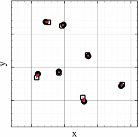
Figure 4. Particle images of  (hollow squares) and
  (full circles) and disparity vectors (in red).
Download figure:
Standard imageThe histogram of the disparity vector component is shown in figure 5 (for the sake of clarity, a region containing more particles than that shown in figure 4 is considered in the histogram). For a sufficiently large number of particles within the window (typically above 6), a statistical analysis of the disparity vector dispersion becomes possible.
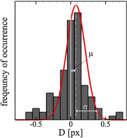
Figure 5. Distribution of the disparity vector.
Download figure:
Standard image2.2.4. Statistical analysis of disparity vector ensemble
Let us assume for simplicity that the components of the disparity set are statistically independent and that they are randomly distributed around the zero. The error committed on each particle pair can be propagated to that of the ensemble considered by the cross-correlation operator. In the hypothesis of a Gaussian distribution of the disparity, the error scales with the standard deviation σ = {σu, σv} of D, and is inversely proportional to the square root of the number of particle pairs N. Therefore, the random error can be estimated as  (Coleman and Steele 2009).
In the more general case, the mean of the disparity set µ = {µu, µv} may be nonzero, when detectable bias errors are present (figure 5).
When the values of µ and σ are computed as the arithmetic mean and the standard deviation of the disparity set, all particles are assumed to make the same contribution to the correlation peak. However, brighter particle images have larger contribution than dimmer ones. This is taken into account by computing µ and σ as weighted mean and standard deviation of the disparity set; the weight is chosen equal to the square root of the particle image intensity product Π:
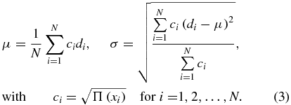
In conclusion, the expression of the instantaneous error estimation  reads
reads
 represents the estimation of the magnitude of the actual error δ on the velocity vector. Expression (4) may be interpreted as follows: in the case of negligible dispersion of the disparity set, the error will be mostly due to the systematic error µ. This is for instance the case when very large interrogation windows are used and N is very large. It should be remarked here that the term µ does not include all possible sources of bias error. In particular, when the measurement is affected by peak-locking, the super-resolution approach is not able to detect the bias error because also the position of the individual particle images is 'locked' at integer pixel positions. In contrast, when the systematic error µ is negligible, the error is dominated by the dispersion of the disparity vectors and decreases with the square root of the number of particle pairs.
The error estimation  can be employed to determine a confidence interval (expanded uncertainty U) about the measurement result which contains the measurand at a given confidence level; this is done by multiplying
  by a coverage factor k:

Coleman and Steele (2009) report that the variable  as computed in (4) is not normally distributed, but rather follows the t distribution with N – 1 degrees of freedom. Therefore, for small N (typically about 20) as occurring in conventional PIV interrogation, 95% confidence level is achieved with k ≈ 2.1 (Coleman and Steele 2009).
The computational cost of the uncertainty quantification depends on the number of particle images in the recordings and is typically about 10% of that of the vector computation.
In summary, the overall procedure can be schematically visualized by the following flow-chart (figure 6).
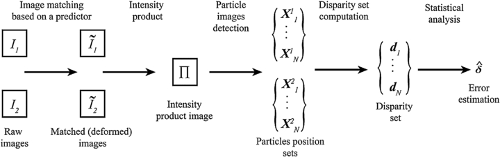
Figure 6. Scheme of the procedure for uncertainty quantification by image matching.
Download figure:
Standard image3. Numerical assessment
Synthetic images of 400 × 400 pixels are generated with a random distribution of 16 000 particles (seeding density of 0.1 particles per pixel (ppp)). The image intensity is rounded off with 8 bit quantization (0–255) and the particle images are assumed to follow a Gaussian shape with 2 pixel mean diameter and 0.2 pixel standard deviation. A Gaussian-shaped laser sheet is simulated having width Δz = 30 pixels. The camera read-out error is modeled as white noise of average intensity equal to five counts; the pixel fill factor equals 1. A uniform displacement is considered with values ranging from 0 to 2 pixels.
The recordings are processed with the three interrogation algorithms introduced in section 2.
- Single–pass.
- Double-step with discrete window offset.
- Multi-step with window deformation (WIDIM).
The window size of 17 × 17 and 33 × 33 pixels is chosen; 50% overlap factor is selected.
A statistical analysis is conducted considering the RMS of both actual and estimated errors:
where the overbar indicates the time average.
The RMS error for single-pass correlation increases linearly in the range of displacement between 0 and 0.5 pixels and stays nearly constant for larger displacements (figure 7). This agrees with well-known results from Westerweel (1993) and Raffel et al (1998). The estimated RMS error from the image-matching technique follows the behavior of the actual error with good accuracy. Oscillations of small amplitude (0.005 pixels) of  RMS about the actual value have a wavelength of 1 pixel and are ascribed to numerical errors associated with the particle image peak fit algorithm. This simple test already shows that the
  scaling correctly takes into account the statistical properties of the error dispersion.

Figure 7. RMS error as a function of the in-plane displacement for different interrogation algorithms. Top-left: single-pass correlation; top-right: double-step cross-correlation with discrete window offset; bottom: multi-pass cross-correlation with window deformation. The symbol key applies to all three plots.
Download figure:
Standard imageThe discrete window offset method introduces a periodic behavior of the RMS error in agreement with the early simulations of Scarano and Riethmuller (2000). The error increases for a displacement increasing from 0 and 0.5 pixels and decreases in the range of 0.5–1 pixels. Also in this case the proposed method yields an accurate error estimate, with discrepancy between  RMS and δRMS of less than a hundredth of a pixel.
The image deformation technique further lessens the random errors, which agrees well with the abundant literature on the subject (Lecordier and Trinité (2003), Scarano (2002), Astarita and Cardone (2005), Fincham and Delerce (2000), among others). In the present test, the actual RMS error does not exceed 0.02 pixels for the smallest window. In this case, the error is clearly overestimated by 30% to 50% due to the limited precision of the individual particle image peak fit (Astarita and Cardone 2005). A minimum error level is thus introduced which may be regarded as a 'fog level' for the present estimator and is considered to be approximately 0.005 pixels.
Again, the scaling with the interrogation window size (namely  ) is reproduced correctly and agrees fairly well with known results (Raffel et al (1998) among others).
The analysis in the remainder does not consider the single-pass cross-correlation method. Therefore, only two techniques are taken into consideration: the double-step interrogation with discrete window offset and the multi-step correlation with window deformation (WIDIM). The interrogation window size is kept at 33 × 33 pixels.
3.1. Displacement gradient
A displacement gradient ranging from 0 to 0.2 pixels per pixel is considered here. The displacement RMS error varies over about two orders of magnitude in the analyzed gradient range (figure 8) when the double-step correlation with discrete window offset is employed. This variation is ascribed to the correlation peak broadening that increases with the displacement gradient (Westerweel 2008).

Figure 8. RMS error as a function of the displacement gradient.
Download figure:
Standard imageThe WIDIM algorithm applies in-plane deformation and compensates the gradient effect. As a result, the measurement error is reduced by one order of magnitude. This result agrees well with previous findings (Scarano and Riethmuller 2000).
For the latter interrogation algorithm, good agreement between actual and estimated error is found, as the error levels lie clearly above the fog level. For the technique based on the discrete window offset, the super-resolution approach provides a good error estimate for displacement gradients below 0.1 pixels pixel–1. For even larger values of the displacement gradient, the error is underestimated. This is ascribed to the particle pair detection technique, which finds a pair as long as their disparity does not exceed a particle image diameter. For a value of the gradient (shear rate in this case) of 0.2 pixels pixel–1, the particle disparity at the edge of the window is already 3 pixels, which cannot be retrieved with the current technique. Further improvements would be needed if the method is to be generalized to flows where the value of the gradient exceeds the measurable range of particle disparity.
3.2. Out-of-plane motion
Particle motion through the measurement plane is recognized as one of the main sources of measurement uncertainty (Adrian 1991, Nobach and Bodenschatz 2009). The current simulation considers a uniform in-plane displacement distributed over 0–2 pixels and uniform out-of-plane displacement w ranging from 0 to 0.4 Δz.
The out-of-plane motion causes a variation of the particle images' intensity level and contributes to the measurement errors in several ways.
- At high seeding density, overlapping particle images that vary their relative intensity lead to a biased displacement estimate that depends on particle image intensity, width and overlap, as thoroughly investigated by Nobach and Bodenschatz (2009). This effect alone was reported to cause random error of PIV measurements of the order of 0.1 pixels.
- At low particle image density, the out-of-plane displacement causes a significant reduction of the correlation signal strength: as a result, in real experiments, the correlation peak shape may become strongly affected by camera read-out noise (Raffel et al 1998).
Nobach and Bodenschatz (2009) report an exponential increase of the RMS error with the out-of-plane displacement. The latter is qualitatively retrieved in the present simulation (figure 9). The image-matching error estimator appears to take into account the out-of-plane motions consistently: the reduction of particle image pairs causes a decrease of N, yielding higher measurement error according to the  scaling. For both interrogation methods, the estimated error follows the actual value increase within 0.005 pixel accuracy.
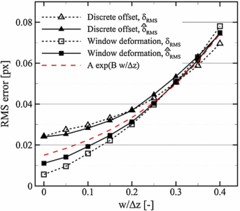
Figure 9. RMS error as a function of the out-of-plane displacement. The red dashed line represents the exponential behavior reported by Nobach and Bodenschatz (2009).
Download figure:
Standard image3.3. Seeding density
Mildly varying planar motion in the range of 0–2 pixels (displacement gradient below 5 × 10–3 pixels pixel–1) is considered here to evaluate the correctness of the estimator with respect to the particle image density. The latter is varied between 0.005 and 0.15 ppp.
The RMS error decreases for increasing seeding density, which is known from previous studies (Raffel et al (1998) among others). When more particle image pairs are present in the interrogation spot, a stronger correlation signal-to-noise is achieved (Raffel et al 1998). The plots of figure 10 show that the scaling rule implied in the model ( ) is consistent with the behavior of the actual error. In particular, one can see that for a four-fold increase of the seeding density the RMS error approximately halves. Also in this case, the agreement between
  RMS and δRMS is within 0.005 pixels.

Figure 10. RMS error as a function of the seeding density.
Download figure:
Standard image3.4. Particle image diameter
The effect of the particle image diameter dτ onto the measurement precision is well known and documented. In the present simulation, particles with an image diameter varying in the range of 0.5–5 pixels are considered. The RMS error for discrete window offset sharply decreases for any increase of the particle image diameter in the range between a fraction of a pixel and 2 pixels (figure 11). For any further increase of dτ, the error increases approximately linearly. This agrees with known results from Westerweel (1997), who reports that peak-locking errors dominate for dτ ≤ 1 pixel and random errors prevail for dτ ≫ 1 pixel. For particle image diameter in the sub-pixel regime, the random errors obtained with window deformation are equivalent to those obtained with the discrete shift technique. When dτ is larger than a pixel, a marked difference is observed: the actual error continues decreasing in the observed range, in contrast with the discrete offset technique. This result is also in contrast with the model recently stated by Westerweel et al (2013) whereby the RMS error always increases with the dτ, irrespective of the interrogation method used for the analysis.
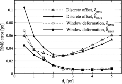
Figure 11. RMS error as a function of the mean particle image diameter.
Download figure:
Standard imageIn this case, the image-matching error estimator shows a marked difference from the actual error when dτ is less than 1 pixel. This result does not come unexpected: in the peak-locking regime also the estimator of the individual particles' peak position is biased to the closest integer. As a result, the estimator is not expected to detect the presence of peak-locking. Nevertheless,  RMS follows the same trend as δRMS and the discrepancy does not exceed 50% for the worst case (dτ = 0.5 pixels). For measurements with particle image diameter of 1 pixel or larger, the error estimator again becomes very accurate.
3.5. Background noise
The effect of the background noise on the measurement uncertainty is evaluated in this section. The main noise sources for conventional CCD and CMOS cameras are classified as follows (http://www.emva.org):
- read noise σr, which appears on each pixel readout and reflects the electronic noise;
- dark noise σd, function of chip temperature, pixel size and exposure time;
- shot noise σs, due to the fluctuations in the number of photoelectrons within a pixel; according to quantum mechanics, the probability of those fluctuations is Poisson distributed, therefore the variance
 of the fluctuations equals the mean number Ne of accumulated electrons.

Following the EMVA standard (http://www.emva.org), a linear model for the camera noise is employed here; therefore the variance of the total noise (expressed in electrons) is calculated as the sum of the variances of each source:

The noise level NL, expressed in counts, is obtained dividing σn by the conversion factor, i.e. the number of electrons per count. Values of NL ranging between 0% and 25% of the maximum particle image intensity Imax are selected, which are considered the standard for state-of-the-art CCD and CMOS cameras used in PIV (Raffel et al 1998).
For both WIDIM and discrete window offset, the RMS error is rather small (below 0.02 pixels) for noise levels below 5%. Larger background noise levels have a detrimental effect on the correlation peak shape (Raffel et al 1998) and cause the RMS error to increase. The uncertainty quantification correctly reproduces the increase of RMS error with background noise (figure 12). Only for high noise level (NL > 20%) is the position of the particle image itself strongly affected by the noise; therefore the accuracy of the uncertainty estimate is reduced.

Figure 12. RMS error as a function of the background noise.
Download figure:
Standard image4. Experimental assessment on a water jet
An established experimental database is used to assess the applicability of the current method in real PIV measurements. The measurements were carried out at the Aerodynamics Laboratories of TU Delft in the Jet Tomography Facility (JTF, Violato and Scarano (2011)). A laminar submerged water jet is issued from a circular nozzle of 10 mm diameter D at 0.45 m s–1 (7 pixels), yielding a diameter-based Reynolds number of 5000. The magnification factor equals 0.44. A sequence of snapshots is recorded with high-temporal resolution (frame rate of 1.2 kHz). In the laminar jet, vortices are shed regularly at a frequency of 30 Hz.
Also in this case, the image-matching uncertainty quantification is considered for images interrogated with window offset as well as window deformation techniques. A window of 33 × 33 pixels is used with 50% overlap factor.
In the present test case, the exact velocity field is unknown. In order to assess the performance of the error estimator, a high accuracy measurement is carried out by processing the recordings with an advanced multi-frame technique, namely the pyramid correlation (Sciacchitano et al 2012). The technique exploits the redundant information of highly oversampled data to reduce the error by an order of magnitude; spatial modulation errors are attenuated via higher spatial resolution, achieved with smaller interrogation windows (17 × 17 pixels). The instantaneous velocity fields measured with the pyramid correlation serve as a reference for calculating the actual error δ. The accuracy of pyramid correlation has been assessed in a previous article (Sciacchitano et al 2012); typical values of the RMS error below 0.01 pixels were obtained. An example of reference velocity field is shown in figure 13(a).
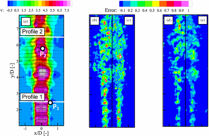
Figure 13. (a) Exact instantaneous displacement field; (b) discrete window offset, |δv|; (c) discrete window offset,  ; (d) window deformation, |δv|; (e) window deformation,
  . Velocity and error are expressed in pixels.
Download figure:
Standard imageTwo regions are identified where the measurement uncertainty is the highest. The first one is the highly sheared region at the jet exit. Here along the shear layer the high measurement error is due to the strong displacement gradient (up to 0.25 pixels pixel–1). The second region is beyond transition, where the turbulent motions cause significant out-of-plane particle displacement.
The analysis with the window offset technique suffers from a significant correlation peak broadening, as also illustrated in the correlation map on the left of figure 14. The resulting measurement errors exceed 0.5 pixels, which is well above the typical figure of 0.1 pixels often considered in the literature as the accuracy of PIV measurements. Similar peak values are also encountered in the turbulent region of the jet.
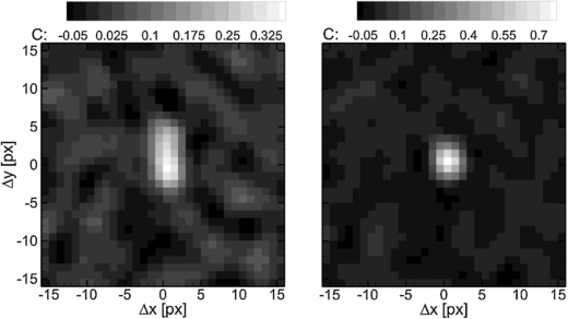
Figure 14. Correlation map along the shear layer (point P1); left: discrete window offset; right: window deformation.
Download figure:
Standard imageThe image-matching error estimator returns a qualitatively similar picture, with peaks along the shear layer near the exit and distributed randomly in the turbulent region.
In figure 13(d, e), the same analysis is conducted with the window deformation technique. In this case the peak broadening is mostly compensated by the in-plane deformation, as confirmed by the correlation map of figure 14 (right). As a result, the measurement error level is about halved. This error reduction is accurately retrieved with the image-matching estimator.
In the turbulent region, where the out-of-plane motion dominates the errors, the measurement error committed with the window deformation is more similar to that of the window offset, though a marked reduction is still observed.
In conclusion, the error committed with each of the interrogation algorithms is estimated consistently with the reference value of the error. Moreover, the estimator identifies the regions of high uncertainty and yields the error magnitude with a relative accuracy of approximately 90% (figure 13).
4.1. Statistical assessment in space domain
A statistical analysis is conducted to quantify the performance of the uncertainty quantification; the RMS error is extracted from two profiles located at y/D = 2.5 and 6.5 respectively. In the laminar flow region (y/D = 2.5), the measurement error is clearly correlated with the in-plane velocity fluctuations; the maximum error occurs at the shear layer locations (figure 15, left). For the discrete window offset algorithm, the high error is ascribed to the correlation peak broadening due to the displacement gradient; the window deformation technique mostly compensates for the displacement gradient, yielding an RMS error reduction by a factor of 3. For both interrogation methods, the estimated error correctly reproduces the actual error behavior within 0.05 pixels.
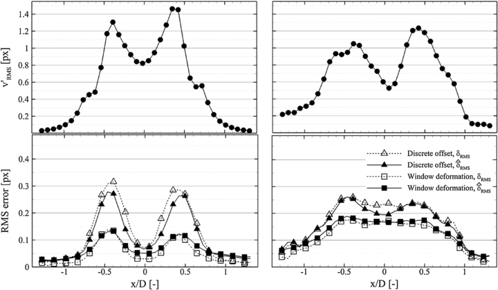
Figure 15. Velocity fluctuations' RMS and RMS error along profiles 1 and 2. Left: profile 1 (y/D = 2.5); top: axial velocity fluctuations' RMS; bottom: RMS error. Right: profile 2 (y/D = 6.5); top: axial velocity fluctuations' RMS; bottom: RMS error. The symbol key applies to both the plots of the second row.
Download figure:
Standard imageIn the turbulent region (y/D = 6.5), the measurement error is ascribed to both in-plane fluctuations (figure 15, top-right) and out-of-plane motion. Due to the turbulent character of the flow, the RMS error profile is approximately uniform inside the jet, as illustrated in the bottom-right plot of figure 15; the error committed with the window offset is slightly larger than that of the window deformation. Also in this flow regime, the agreement between  RMS and δRMS is within 1/20th of a pixel for both interrogation methods.
4.2. Statistical assessment in time domain
A statistical analysis in time domain is conducted to evaluate the performance of the super-resolution approach in estimating instantaneous errors; two points P1 and P2 along the shear layer and in the turbulent region respectively (figure 13(a)) are considered here.
Along the shear layer, the velocity exhibits low frequency fluctuations ascribed to shear layer oscillations (figure 16(a)). When the spatial resolution is insufficient, those oscillations are not accurately captured by the interrogation algorithm and the measurement error assumes periodic behavior, as clearly visible in the plot of figure 16(g), which refers to the WIDIM algorithm. The double-step interrogation with discrete window offset (figure 16(c)) yields additional high frequency measurement errors due to random noise and in-plane displacement gradients, as discussed in the previous sections.
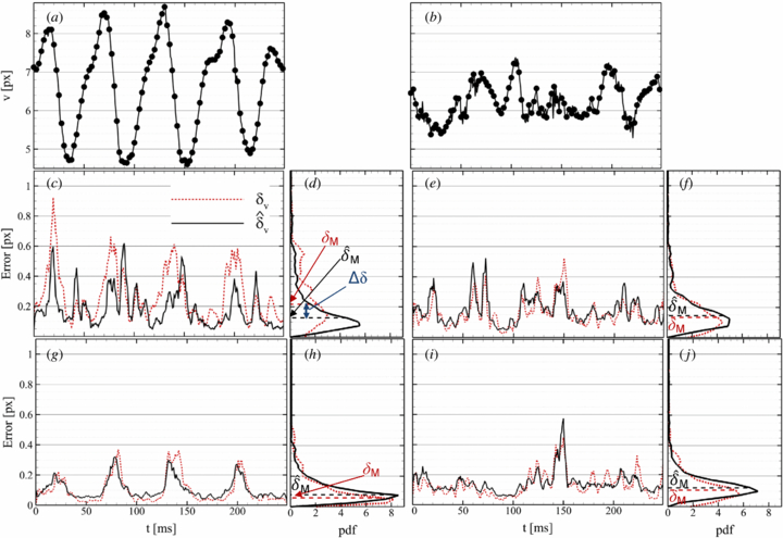
Figure 16. (a) Actual axial velocity in P1. (b) Actual axial velocity in P2. (c) Error time series in P1, discrete window offset. (d) pdf of the error displayed in (c). (e) Error time series in P2, discrete window offset. (f) pdf of the error displayed in (e). (g) Error time series in P1, window deformation. (h) pdf of the error displayed in (g). (i) Error time series in P2, window deformation. (j) pdf of the error displayed in (i).
Download figure:
Standard imageIn the turbulent flow region (point P2, figure 16(b)) the measurement error exhibits high frequency content due to the three-dimensionality of the flow and the unresolved turbulent scales (figures 16(e) and (i)). The error plots of figure 16 highlight the high correlation level between actual and estimated error on the axial velocity component (δv and  v, respectively).
The probability density functions (pdf) displayed in figure 16 show that the measurement error is mainly distributed in the range of 0–0.2 pixels; the relative agreement between the medians of the actual and estimated error (δM and  M, respectively) is within 40% (table 1). The higher discrepancy occurs in the shear layer using the with discrete window offset method (figure 16(d)): in this case, the error is underestimated by about 40%. This is due to the strong displacement gradient (above 0.1 pixels pixel–1) responsible for positional disparities exceeding the particle image diameter, which is not detected with the present approach.
Table 1. Comparison between actual and estimated error in P1 and P2.
| P1 | P2 | |||||||
|---|---|---|---|---|---|---|---|---|
| δM (px) |  M (px) M (px) |
Δδ =  M – δM (px) M – δM (px) |
|Δδ|/δM (%) | δM (px) |  M (px) M (px) |
Δδ =  M – δM (px) M – δM (px) |
|Δδ|/δM (%) | |
| Discrete window offset | 0.218 | 0.130 | –0.088 | 40% | 0.134 | 0.145 | 0.011 | 8% |
| Window deformation | 0.059 | 0.079 | 0.020 | 34% | 0.108 | 0.123 | 0.015 | 14% |
4.3. Uncertainty effectiveness
Timmins et al (2012) introduced the 'uncertainty effectiveness' to investigate the appropriateness of their uncertainty estimation: this parameter is defined as the percentage of calculated vectors V which contain the true value Vactual within their uncertainty band ±U, i.e. such that V – U < Vactual < V + U. Consistent with the analysis of Timmins et al (2012), here the uncertainty  is computed at 95% confidence level; since the average number of particle pairs within a 33 × 33 pixel interrogation window is N = 25, the corresponding coverage factor for 95% confidence level is k = 2.1 (Coleman and Steele 2009).
The uncertainty effectiveness indicates the actual confidence level of the estimated uncertainty: if U has been correctly estimated, the uncertainty effectiveness equals the chosen confidence level. The computed values are tabulated in table 2 for both the interrogation algorithms. For WIDIM, the uncertainty effectiveness shows good agreement with the theoretical value of 95%, confirming the validity of the present approach for error estimation. The image-matching estimator exhibits uncertainty effectiveness above 90% for both radial and axial velocity components.
Table 2. Uncertainty effectiveness for the jet experiment.
| Uncertainty effectiveness on the radial velocity u (%) | Uncertainty effectiveness on the axial velocity v (%) | Theoretical value of the uncertainty effectiveness (%) | |
|---|---|---|---|
| Discrete window offset | 85 | 83 | 95 |
| Window deformation | 94 | 92 | 95 |
Slightly lower values of uncertainty effectiveness are obtained with the double-step correlation with discrete window offset: this may be ascribed to the difficulty of correctly pairing the particle images in the presence of strong in-plane deformation, leading to an underestimation of the true measurement error. However, for both velocity components the uncertainty effectiveness exceeds 80%.
The authors remark that this parameter alone is not sufficient to assess the precision of the uncertainty quantification algorithm: in fact, a very conservative estimation would lead to uncertainty effectiveness values tending to 100%. For this reason, in this work the algorithm's precision has been investigated with a statistical analysis observing both the spatial distribution of the error and its time history at significant locations in the flow domain.
4.4. Example of the uncertainty minimization procedure
Since the measurement error is not known a priori, the investigator is left with empirical procedures to evaluate and minimize it during the processing phase. A typical procedure consists in gradually reducing the interrogation window size; at any reduction step, the spatial resolution increases at the cost of an increase of the measurement noise. The interrogation window is selected as the smallest window providing a noise level considered acceptable. Clearly, such a procedure is largely dependent on human perception of the measurable signal and the embedded noise and does not guarantee that the interrogation window choice is actually optimal. The image-matching error estimator can be used to select the window size in a rigorous way in order to minimize the measurement uncertainty.
As an example, a region of the jet is processed with WIDIM with interrogation windows from 61 × 61 to 11 × 11 pixels (figure 17). By eye inspection of the instantaneous velocity fields (first row of figure 17), the investigator gets the impression that large interrogation windows yield strong modulation effects, whereas small windows largely increase the measurement noise. This is confirmed by the error analysis conducted in the second row of figure 17: the interrogation window of 11 pixels shows high errors not only in the shear layer, but also in the jet core and in the quiescent region due to the high noise level; in contrast, the 51 × 51 window yields low uncertainty outside the jet due to the high measurement robustness, but causes high modulation errors in the shear layer. In this case, the window of size 31 × 31 pixels minimizes the measurement error. For the different window sizes, the agreement between actual and estimated error is within 40%.

Figure 17. First row: instantaneous velocity field; second row: RMS error at the different window sizes; (a) 11 × 11 pixels, δRMS; (b) 11 × 11 pixels,  RMS; (c) 31 × 31 pixels, δRMS; (d) 31 × 31 pixels,
  RMS; (e) 51 × 51 pixels, δRMS; (f) 51 × 51 pixels,
  RMS. The velocity and the error are expressed in pixels.
Download figure:
Standard imageThe RMS error in the points P1 and P2 previously defined (figure 13) is considered to determine the optimal window size. The plots of figure 18 show the importance of a correct choice of the interrogation window, which allows the measurement error to be reduced by a factor of 2.

Figure 18. RMS error on the axial velocity component; left: point P1; right: point P2. The symbol key applies to both plots.
Download figure:
Standard imageIn the shear layer (point P1, figure 18, left), the measurement error exceeds 0.1 pixels for windows larger than 45 × 45 pixels: this finding is consistent with well-known results reported in the literature (Raffel et al (1998) among others), which indicate that large windows are strongly affected by displacement gradients. The error is reduced down to 1/20th of a pixel using windows of size between 30 × 30 and 40 × 40 pixels.
In the turbulent region (point P2, figure 18, right) the out-of-plane motion largely reduces the correlation signal strength for windows below 20 × 20 pixels, causing errors above 0.15 pixels. In this case, the measurement error is reduced by a factor of 2 using windows larger than 30 × 30 pixels, which increase the correlation signal-to-noise ratio.
From the present analysis, the measurement error of the jet experiment is minimum when the interrogation window is selected in the range from 30 × 30 to 40 × 40 pixels. For all window sizes, the estimated error follows the actual value within 0.05 pixels.
5. Summary and conclusions
The image-matching uncertainty quantification is introduced to estimate local error in planar PIV data. The approach is a posteriori, meaning that the measured velocity field is used as input along with the original images to quantify the uncertainty of the velocity field itself. The working principle is general and can be applied to any single-pair interrogation algorithm based on cross-correlation. The principle of the method relies on the concept of super-resolution: the image pair is matched according to the cross-correlation analysis and the residual distance between matched particle image pairs (particle disparity vector) due to incomplete match between the two exposures is measured. The ensemble of disparity vectors within the interrogation window is analyzed statistically to infer the instantaneous uncertainty of the measured displacement. The method accounts for random errors and systematic errors due to spatial modulation; in contrast, peak-locking errors and truncation errors in time are not detected with the present approach.
The performance of the image-matching uncertainty quantification is assessed via Monte Carlo simulation. The interrogation methods employed for the analysis range from simple ones (single-pass correlation, double-step with discrete window offset) to the state-of-the-art of PIV interrogation (multi-step with window deformation). The error associated with several measurement conditions, such as in-plane and out-of-plane displacement, in-plane displacement gradient, particle image diameter and seeding density, is investigated. The estimated RMS error follows the behavior of the actual error with accuracy in most cases within a hundredth of a pixel; also the validity of our model based on the  scaling is proven. As expected, the present approach shows its limitations for particle images having diameter of 1 pixel or below; in this case, the particle image position is affected by peak-locking errors and leads to lower accuracy in the estimated error.
Water jet measurements are considered for the experimental assessment. High accuracy displacement fields serving as ground truth are built with an advanced processing technique, namely the pyramid correlation (Sciacchitano et al 2012). The performance of the image-matching uncertainty quantification is evaluated observing both the spatial distribution of the error as well as its time history at relevant locations in the flow domain. It is shown that the estimator is suitable to quantify a posteriori the measurement uncertainty from real experiments with accuracy exceeding 60%. The authors claim that this is a major achievement for PIV, because it constitutes the basis for quantifying the uncertainty of statistical quantities such as means, variances and Reynolds stresses, which are of paramount interest in the investigation of turbulent flows.
An important outcome of the image-matching uncertainty quantification is the possibility to minimize the measurement uncertainty in the processing phase. An example of the uncertainty minimization procedure is presented: the recordings are processed with several window sizes and the optimal interrogation window is selected as that minimizing the estimated measurement error. It is shown that a correct choice of the interrogation window size may yield a measurement error reduction by a factor of 2.