
Abstract
We present molecular dynamics (MD) simulations of the formation of 2D materials with a honeycomb structure from 2D simple monatomic liquids with honeycomb interaction potential (Rechtsman et al 2005 Phys. Rev. Lett. 95 228301). Models are observed by cooling from the melt at various cooling rates. Thermodynamics of the phase transitions is analyzed in detail. Depending on the cooling rate, amorphous or crystalline honeycomb structures have been found. Structural properties of the crystalline honeycomb structure are studied via radial distribution function (RDF), coordination number and ring distribution, including 2D visualization of the atomic configurations. We find evidence for the existence of polycrystalline honeycomb structures and new structural defects, not previously reported. The atomic mechanism that forms the solid phase of a honeycomb structure from the liquid state has been analyzed by monitoring the spatio-temporal arrangement of atoms in 6-fold rings and/or atoms with the coordination number  , occurring upon cooling from the melt. Since knowledge of how real 2D solids with honeycomb structures form from the vapor or liquid phase is still completely lacking, our simulations highlight the situation and give a deeper understanding of the structure and thermodynamics of real 2D materials such as graphene, silicene, germanene, etc.
Export citation and abstract BibTeX RIS
1. Introduction
In recent years, 2D materials with honeycomb structures (flat or buckling), such as graphene, silicene, germanene ..., have been under intensive investigation due to their enormous fundamental and technological importance [1–9]. Graphene can be synthesized by various techniques, including mechanical exfoliation, thermal chemical vapor deposition, plasma-enhanced chemical vapor deposition, thermal decomposition of SiC, thermal decomposition on other substrates, un-zipping CNTs [3–5], or even growth from a molten phase [6]. However, our knowledge of graphenization (e.g. the formation of graphene from vapor or the liquid phase) is still completely lacking [4]. The same situation remains for other 2D materials. In order to understand the atomic mechanism of graphenization, information at the atomistic level is required and computer simulations can provide such detailed information. However, we can find no simulation study carried out in this direction. Attention has, instead, been paid to calculation of the intrinsic ripples in graphene, the temperature dependence of various mechanical properties, electronic structure, etc [7, 10–12]. Note that the electronic, thermal and mechanical properties of graphene are very sensitive to lattice imperfection and the latter depends on the synthesis method. Although various types of structural defect in graphene have been proposed and summarized [5], its defects and their dynamics remain experimentally unexplored. Moreover, small graphene models of the first principle calculations cannot provide a full picture of structural defects in material [5, 13, 14]; this requires analysis of structural defects existing in large graphene models, obtained by MD simulation. It is of great interest if we have a simple monatomic model which yields the formation of a honeycomb structure. This allows one to carry out a comprehensive MD simulation of the formation of a 2D honeycomb structure from the liquid state, including the thermodynamics of the phase transition and detailed analysis of structural properties. Using a simple monatomic model for such a purpose one has an advantage since one can focus attention only on the topology of atomic arrangements related to the phase transition, rather than on both topological and chemical bonding, if one uses a binary system. In addition, calculations using simple monatomic models should not be time-consuming compared to those with realistic interatomic potentials. Such a potential indeed exists. A honeycomb pair interaction potential, which yields the 2D honeycomb structure, has been proposed [15] and subsequently checked carefully by a group at Princeton University [16–19], and recently by Zhou [20].
However, relatively small models have been used for checking (containing 400–500 atoms) so that a little information about the models has been found [15–19]. On the other hand, there is no comprehensive simulation of a formation of honeycomb structure from the melt and we also have no detailed information of structure which includes various structural defects. Therefore, our main aim here is to carry out a comprehensive MD simulation in this direction in order to clarify the situation, not only for the honeycomb structure but also for recently discovered 2D materials such as graphene, silicene etc., which also have a honeycomb structure (flat or buckling).
2. Calculations
Formation of 2D simple monatomic models with honeycomb structure from a 2D liquid state containing 16 428 atoms has been studied by MD simulation. The honeycomb pair potential used in the present work has the form given below [15]:
This potential has two minima, the shallow one is located at  in the positive region of potential and the deeper minimum is located at
  in the negative region of potential [15]. Initial flat 2D atomic configurations with simple square lattice structure of size
  and at the density
  have been relaxed at a temperature as high as
  for 106 MD steps in order to get a good equilibrium liquid state. We use
  ensemble simulation and periodic boundary conditions (PBCs). Here,
  and
and  is the distance between atoms and
  is the diameter of an atom. The density
  is adopted in order to get a final honeycomb structure like that proposed in [16]. Via Monte-Carlo simulations it is found that, depending on the temperature and density used in simulations, various phases of 2D systems with honeycomb potential can be obtained and the phase diagram in the reduced density-reduced temperature T representation can be seen in [16]. In the low temperature region, at the density
  a triangular phase is formed, the nearest-neighbor distance being approximately 1.84, which corresponds to the location of the deeper minimum in the interaction potential at
  . If density is increased to
  , the honeycomb crystal becomes stable because it's nearest neighbors are at the distance
  , close to the shallow minimum at
  , and the next nearest neighbors at the distance
  , close to the deeper minimum at
  (see more details in [16]). Following Lennard-Jones, reduced units are used in the present work: the length in units of
  , temperature
  in units of
  , and time in units of
  where
where  is the Boltzmann constant and
  is an atomic mass. The Verlet algorithm is employed and the MD time step is
  . We take the same cutoff for potential at
  as that done in [15] and [16]. Then the system is cooled down at a constant volume while the temperature is decreased linearly with time as
  via the simple atomic velocity rescaling until reaching
  . Here,
  is a cooling rate and
  is the number of MD steps. Five different cooling rates have been used, as follows:
  per MD step with
  ranged from 5 to 9. In order to improve the statistics, we average results over five independent runs. In order to calculate coordination number distribution, the cutoff radius
  is taken which is equal to the position of the first minimum after the first peak in the RDF of the model obtained by cooling the cooling rate of
  per MD step at
  . Indeed, we also find that the position of the first peak in the RDF (or the bond length) at the same cooling rate, and at
  , is equal to around
  , as discussed above.
Note that a more complicated pair potential, which also yields a 2D honeycomb structure, has been proposed recently [21, 22]. However, we adopt the potential presented in equation (1) for simulations due to its simplicity. On the other hand, we use VMD software [23] for 2D visualization of atomic configurations in the paper and LAMMPS for MD simulations [24]. Note that the honeycomb interatomic potential presented in equation (1) has not been implemented in LAMMPS yet and, therefore, it has been given in the form of a table of values stored in one of the input files. We employ ISAACS software for calculating ring statistics following the 'shortest-path' criterion for definition of rings (see [25] and references therein).
3. Results and discussions
3.1. Thermodynamics and structure evolution upon cooling from the melt
As shown in figure 1, as is commonly found for 3D systems, at the first two highest cooling rates the change of total energy upon cooling from the melt is rather smooth, indicating a glass transition in the system (the upper curves in figure 1). However, discontinuity of temperature dependence of total energy at lower cooling rates exhibits a first-order behavior of the phase transition, i.e. crystallization occurs in the system (figure 1). Note that potential of equation (1) has two wells [15]: the first is located at the position of positive value of potential and atoms; our models mainly concentrate on this well-yielding positive value for the total energy presented in figure 1. On the other hand, temperature dependence of the heat capacity for models obtained at the highest and lowest cooling rates exhibits a single peak, which can be considered to be glass transition and crystallization temperatures, i.e.  and
and  respectively (figure 2). The heat capacity has been found approximately via the simple relation:
  ,
,  , which is the discrepancy of the total energy between
  and
and  on cooling. Note that temperature dependence of the heat capacity presented in figure 2 is used only for determination of the phase transition temperature. Glass formation or crystallization of the system can be seen via RDF of the models obtained at five different cooling rates and at temperatures as low as
  (see figure 3). Indeed, smooth RDF of the models obtained at the high cooling rates of
  and
and  per MD step indicates a glass structure in the models. By contrast, additional peaks occur in the RDF of the models obtained at lower cooling rates, indicating crystallization (fully or partially) of the system. At the lowest cooling rate,
  per MD step, total energy has a sudden drop at around the freezing temperature and exhibits a first order-like behavior of the phase transition. On the other hand, since glass transition in the supercooled 2D honeycomb structure-forming liquids is of great interest, and this is a big topic, we leave it for detailed analysis in our subsequent paper.

Figure 1. Temperature dependence of total energy of the system upon cooling from the melt at various cooling rates.
Download figure:
Standard image High-resolution image
Figure 2. Temperature dependence of the heat capacity of the system upon cooling from the melt at the lowest and highest (inset) cooling rates.
Download figure:
Standard image High-resolution image
Figure 3. Radial distribution function at  for models obtained at five different cooling rates.
Download figure:
Standard image High-resolution imageIt is of interest to see the evolution of the structure upon cooling from the melt (figure 4). We show the RDF of temperature ranged from  to 0.1 with decrement of 0.1. One can see that at high temperature, the RDF is rather smooth and the height of its peaks is small, exhibiting a clearly liquid-like behavior. However, upon cooling from the melt the height of the first and second peaks is enhanced. At around the crystallization temperature (
 ), additional peaks appear, indicating crystallization of the system, and multi-peak RDF at
  exhibits clearly the crystalline behavior of the system at low temperatures. The evolution of the structure of the system can be seen clearly via evolution of the mean coordination number and mean ring size in the system, obtained at various cooling rates (figure 5). One can see that in the liquid state the mean coordination number is equal to around 3.8–3.9, and it decreases down to around 3.00 and 3.45 for the lowest and highest cooling rates at
  respectively. It is clear that low-coordinated crystal with honeycomb structure formed at the lowest cooling rate has the mean coordination number
  like that found for an ideal honeycomb structure. However, coordination number distribution shows the existence of various defects in the obtained models which will be analyzed in detail below. Moreover, temperature dependence of the mean coordination number of models obtained at the lowest cooling rate has a sudden drop at freezing temperature, which exhibits a first-order behavior of transition in the system like that discussed above. On the other hand, evolution of the mean coordination number in the models obtained at the highest cooling rate is rather smooth, indicating liquid-glass behavior of the transition (figure 5). Mean coordination number
  for the glassy state obtained at
  and at the highest cooling rate, indicates a strong distorted honeycomb structure with a large amount of structural defects compared to that of the ideal crystalline honeycomb structure.

Figure 4. Evolution of radial distribution function upon cooling from the melt at the cooling rate of  per MD step (from top to bottom: for temperature ranged from T = 1.0 to 0.1 with decrement of 0.1). The bold line is for
  which is close to
  .
.
Download figure:
Standard image High-resolution image
Figure 5. Evolution of mean coordination number and mean ring size (inset) upon cooling from the melt at five different cooling rates.
Download figure:
Standard image High-resolution imageIn addition, the decrease in the mean coordination number in the honeycomb structure-forming system upon cooling from the melt (or increase upon heating from low temperature state, see figure 5) may be related to the negative thermal expansion coefficient (TEC) of our 2D honeycomb structure model. Notice that a negative TEC of graphene has been observed by both experiments and computer simulations [10, 26–28]. Indeed, Monte-Carlo simulations show that graphene models have a negative TEC in the range 0–300 K and after that it becomes positive [10]. By contrast, the TEC of graphene, as a function of temperature, is estimated by using a first-principle calculation which finds that it is negative for the whole temperature range studied, up to 2500 K (see [26]). However, it is found experimentally that the TEC of graphene is negative just for the temperature range 300–350 K [27] or 200–400 K [28]. The reason for the discrepancy between calculations and experimental data is still unclear; it may be related to uncertainties in the accuracy of the experimental measurements or to a limitation of the computer simulations. Further studies are needed in order to clarify the situation. Decrease of the mean coordination number of our honeycomb structure-forming 2D system, for the whole temperature range studied, ranged from the normal liquid state to a solid honeycomb structure, is anomalous and unlike that commonly found for 3D systems. It is of great interest to check the problem for a more realistic model, such as graphene with a realistic interatomic potential. It is suggested in [26] that the anomaly, i.e. a negative TEC of graphene, is due to a low-lying bending phonon branch [29].
An opposite tendency has been found for evolution of the mean ring size in the system upon cooling from the melt compared to that of the mean coordination number (see the inset of figure 5). We find that rings almost have not been formed in the high temperature liquid state and a significant amount of rings occurs at temperatures just above freezing (i.e. at around  , see the inset of figure 5). However, further cooling leads to a strong increase of the mean size of the rings. At the lowest cooling rate, the mean size increases suddenly at freezing temperature, reaching a value of around 5.97, which is very close to the 6-fold ring of the ideal honeycomb structure. A small deviation from the 6-fold ring indicates the existence of the defective rings in the system, compared to the ideal honeycomb structure. Moreover, a sudden increase of the mean size of a ring at freezing temperature in models obtained at the lowest cooling rate, also exhibits a first-order behavior of the phase transition like that discussed above. By contrast, evolution of the mean size of rings in models obtained at the highest cooling rate is rather smooth, indicating the glass transition in the system upon cooling from the melt. Again, mean size of ring in the glassy state is equal to around 4.7 (i.e. strong deviation from the value 6.0 for an ideal honeycomb structure), which is related to a large amount of structural defects in the amorphous honeycomb structure.
3.2. Structure of crystalline honeycomb state at low temperature
We stop here for a detailed analysis of the structure of a crystalline honeycomb state obtained at  and at the lowest cooling rate of
  per MD step: i.e., we deal with the crystalline honeycomb structure. Note that the configurations have been relaxed for
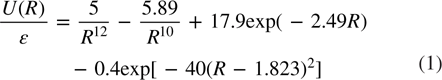
  MD steps before analyzing the structure. First, via the coordination number distribution presented in figure 6 one can see that about 98% of atoms in the crystalline honeycomb structure have
  and about 2% of atoms also have
  and
and  , indicating the existence of structural defects in the system with a small fraction. However, more details of structural defects in the models can be seen via the ring distribution (see the inset of figure 6). Indeed, about 95% of rings are 6-fold and the percentage of the remaining rings is around 5%. One can see that the ring distribution of 2D crystals with a honeycomb structure obtained by cooling from the melt is rather wide, ranged from 3-fold to 13-fold rings. However, the fraction of rings larger than nine members is too small, i.e. less than
  , and it has not been shown in the inset of figure 6. We can take the data for graphene, a real 2D material with honeycomb structure, in order to compare. 95% of rings are 6-fold, confirming again that hexagonal rings serve as the building blocks of crystalline graphene [1]. 5-fold and 7-fold rings can be considered as defects derived from the corresponding two 6-fold rings; they may relate to the Stone-Wales defects often mentioned for graphene [5, 13, 14] or to the grain boundary (GB) of polycrystalline honeycombs, since experiments revealed that the grains stitch together predominantly via pentagon–heptagon pairs (see [30] and references therein). 8-fold rings have been also mentioned for graphene and it may relate to the di-vacancies which can be created either by the coalescence of two single vacancies or by removing two neighboring atoms [5]. Note that presence of 4-fold rings in graphene has been highlighted by TEM study, proposed as the result of overlapping the two pentagons of the adjacent di-vacancies [14]. Finally, 3-fold rings found in the present work are related to the so-called adatom defects (see figure 7 and discussions given below). Existence of 3-fold rings in graphene has been rarely mentioned in the literature, although one can see them in MD simulation models [31]. It was found that in an amorphous SiO2 surface, 3-fold rings are more active than larger rings for the surface reactivity (see for example, [32]); the same situation for 3-fold rings in graphene can be suggested.
Figure 6. Coordination number distribution and ring statistics (inset) in models obtained at  and at cooling rate of
  per MD step.
Download figure:
Standard image High-resolution image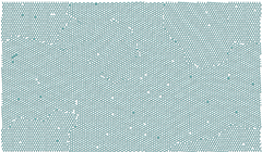
Figure 7. 2D visualization of the well-relaxed atomic configuration of model obtained at the lowest cooling rate of  per MD step at
  .
.
Download figure:
Standard image High-resolution imageThe nature and existence of 3-fold rings in our honeycomb structure can be seen via 2D visualization of the obtained models given below. The existence of 9-fold rings has been speculated previously for graphene [5] and is found in the present work. However, their fraction is too small. Some extra-large member rings found in our crystalline honeycomb structure can be seen in figures 8(a) and (b), including those with the dangling bond. Generally, multi-member rings lead to the formation of vacancies of various unusual shapes which have not been mentioned for graphene in the past [5, 13, 14]. The rings that differ from 6-fold rings can be considered as structural defects; it has been found that they can exhibit chemical reactivity which is higher than that of 6-fold rings [13]. In particular, for Stone-Wales defects and bi-vacancies, the chemisorption energy of a single hydrogen atom on these defects is negative, making such defects centers of a stable chemisorption of hydrogen [13].
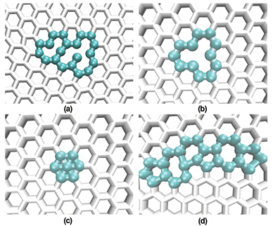
Figure 8. Some structural defects of the crystalline honeycomb models: (a) unusual-shaped vacancy formed by multi-member rings; (b) monovacancy; (c) adatom; (d) part of the grain boundary.
Download figure:
Standard image High-resolution imageStructural defects in graphene, which may appear during growth or processing, are of great interest, since they may deteriorate the performance of graphene-based devices and/or become useful in some applications [5, 13, 14]. In order to see more clearly other types of defects of the obtained honeycomb structure, we show a 2D visualization of the models obtained at the lowest cooling rate of  per MD step and at
  in figure 7. Note that the models have been relaxed for
  MD steps before visualization in order to get a good equilibrium. Some important points can be drawn, as follows:
- (i)There is evidence of the existence of GB of polycrystalline structure (it can be seen clearly around 04 corners in figure 7 although we have no full GB), which has not been mentioned in the small models previously reported by ab initio calculation. However, the size of our models should be larger in order to see some full domains. Polycrystalline graphene has been under intensive investigation by both experiment and computer simulation in recent years [30, 33–36]. Indeed, large graphene models (containing 138 000 and 278 000 atoms) contain a significant amount of grains [30]. Polycrystalline graphene has been considered as a patchwork of coalescing graphene grains of varying lattice orientations and size, resulting from the chemical vapor deposition (CVD) growth at random nucleation sites on the metallic substrates [30]. As a result, GB should dictate various properties of graphene including electrical transport ones of CVD graphene [35]. Since the properties of polycrystalline materials are dictated by their grain size and by the atomic structure at the grain boundaries, it is of great interest to carry out the study in this direction. The structure of the grain boundaries will be discussed below since it is related to various defects.
- (ii)Various structural point defects have been found in our crystalline honeycomb structure, including ones previously unreported in the literature (figures 7 and 8). First, one can see in figure 7 that mono- or multiple vacancies are abundant in the models, such as those found through both experiment and computer simulations for graphene [5]. Computer simulations have found that di-vacancies (and/or multiple ones) are thermodynamically favored over single vacancies, and migration of di-vacancies (and/or multiple ones) needs an activation energy which is much higher than for a single one [5]. This makes di-vacancies immobile up to very high temperatures, at which these vacancies could migrate either by atom jumps or by switching between different reconstructions [5, 37]. Di-vacancies can be created by the coalescence of two single ones or by removing two neighboring atoms. Removing more than two atoms may lead to larger and more complex defect configurations like that suggested in [5]. Indeed, it is found in our present work (figures 7 and 8). Vacancies in models obtained by cooling from the melt are rich of various sizes and shapes which have not been previously reported (see figures 7 and 8) and they may act as reactive sites for various physico-chemical performance of 2D materials in general [13]. Second, we find the existence of the so-called 'adatom' defects (figure 8(c)), i.e. like interstitial atoms in 3D crystals, with a significant amount in our 2D models. It is suggested that 'adatoms' do not exist in graphene, i.e. placing an atom to any in-plane position—in the center of a hexagon would require a prohibitively high energy [5]. It was further speculated that the energetically favored position for this case is the bridge configuration, i.e. an adatom is located on top of the C-C bond [5]. However, significant amounts of adatoms exist in our honeycomb structure, indicating that the situation may be quite different from that stated previously [5], especially for graphene synthesized by the vapor deposition on substrate. Indeed, it requires very high energy for the formation of the adatoms in the solid state like that discussed in [5]. However, it is possible that the formation occurs in the liquid state (i.e. in the region not far above freezing point) since it should not require high formation energy for the formation of adatoms in the liquid state. Note that our honeycomb structure has been obtained by cooling from the melt, and adatoms indeed occur in the liquid state in the temperature region close to freezing point and then freeze upon further cooling (not shown). This means that adatoms are not artificial results due to the 2D simulation setup but should be the result of a preparation method. In practice, adatoms should be formed if graphene is synthesized by CVD or by quenching the system from the melt. Adatoms could not be formed in graphene obtained by mechanical exfoliation from graphite. Concerning stability of the adatoms, we can check it via DFT calculations for a realistic model, i.e. for graphenization of 2D liquid carbon. However, we find that adatoms are rather stable for a relatively long MD relaxation at a given temperature (for more than 105 MD steps of relaxation, not shown). Moreover, adatoms also have a tendency to coalesce to form a new defect composed of several adatoms (see the upper left corner of figure 7). Note that the concept of what are typical defects in the real graphene samples and their concentrations is still unclear. Our simulations give additional understanding of the situation. However, it should be checked for the 'real models' of graphene which would be obtained by cooling from 2D liquid carbon with a realistic interatomic potential. On the other hand, one can see that adatom defects yield the occurrence of 3-fold rings in our models like that found and discussed above.
- (iii)We stop here for discussion about structure of GB of the honeycomb structure observed. It is found by both experiments and computer simulations that GB of polycrystalline graphene consists predominantly of 5- and 7-fold rings [30]. This may be partially true (see figures 7 and 8(d)) since we find that GB contains 5- and 7-fold rings including Stone-Wales type defects. However, as shown in figure 7 , GB contains not only 5- and 7-fold rings but also various defects, such as multi-member-rings, various vacancies and adatoms in combinations. As discussed above, larger models should be taken in order to study a full polycrystalline honeycomb structure, especially for the 'real' models of graphene.
Based on the analysis presented above one can see that a crystalline honeycomb structure obtained by cooling from the melt is filled with Stone-Wales defects, polygonal rings, various point or even line defects like that commonly found for crystalline graphene [5]. However, we find several new insights related to the defects in the 2D honeycomb structure, which have not been previously reported (see our discussions given above). It is well known that defects of graphene are centers for impurities with an enhanced chemical activity [13, 38]. In particular, defect sites are more reactive for OH adsorption but play different roles, i.e. for example, while OH adsorption at single vacancy is highly dissociative Stone-Wales defects could stabilize the OH groups on the graphene basal plane [38]. As shown above, GBs consist of various types of defect in a honeycomb structure, including vacancies, Stone-Wales type defects and multi-member rings; therefore, GB of polycrystalline graphene may act as the region for impurities and chemical activity of 2D materials.
3.3. Atomic mechanism of honeycomb structure formation
As discussed in the Introduction, although graphene (and/or other 2D materials with honeycomb structure) have been synthesized by various techniques including CVD and growth from the molten state, our understanding of the formation of solid honeycomb structure from the liquid or vapor state is still completely lacking. We try to highlight the situation. Since 6-fold rings are the building blocks of graphene (and/or other 2D materials with honeycomb structure), it is worth monitoring the occurrence and subsequent growth of atoms involving 6-fold rings in the system upon cooling from the melt. On the other hand, a perfect crystalline honeycomb structure has atoms with coordination number  , and therefore, it is also of great interest to see the evolution of the fraction of atoms with
  occurring in the system upon cooling from the melt. The atomic mechanism of honeycomb structure formation can be monitored via analysis of the spatio-temporal arrangements of atoms involving 6-fold rings and/or atoms with
  occurring in the system upon cooling from the melt. As seen in the inset of figure 5, the formation of a solid honeycomb structure in our models is indeed related to the sudden increase of fraction of 6-fold rings at the freezing point. The same tendency has been found for the fraction of atoms with
  (figure 9). Therefore, it is quite true if we go on by this way, i.e. analyzing spatio-temporal arrangements of atoms involving 6-fold rings and/or atoms with
  in order to get information related to the formation of solid honeycomb structure from 2D liquids.
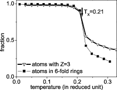
Figure 9. Temperature dependence of fraction of atoms involving in 6-fold rings and atoms with  in models obtained at the cooling rate of
  per MD step. Statistical error is smaller than the size of scattering symbols.
Download figure:
Standard image High-resolution imageOne can see in figure 9 that the temperature dependence of the fraction of atoms involving 6-fold rings is similar to that of the mean size of rings in models obtained at the lowest cooling rate, presented in the inset of figure 5. That is, a very small fraction of atoms with 6-fold rings has been found at temperatures just above freezing point and further cooling leads to the intensive increase of the fraction of these atoms (figure 9). A sudden increase of atoms involving 6-fold rings, or atoms with  , occurs at around the freezing temperature. At the freezing temperature (i.e. at
  ), 83% of atoms in the system are involved in 6-fold rings (or atoms with
  ) to form a relatively rigid honeycomb structure. A full honeycomb structure is formed at a temperature just below
  . Notice that a similar high fraction of atoms involved during the solid-like formation phase has been found for freezing of a 3D system with Lennard-Jones-Gauss potential (i.e. around 75% atoms become solid-like at the freezing temperature, see [39]). One can see that the temperature dependence of the fraction of atoms with
  is the same as that found for atoms with 6-fold rings (figure 9). We show a 2D visualization of the occurrence of atoms with
  in figure 10 in order to see more details of the formation of the solid honeycomb structure in the system upon cooling from the melt. We take 2D atomic configurations at three different temperatures close to the freezing region, where the fraction of atoms with
  starts to strongly increase to form a rigid honeycomb structure (figures 9 and 10). One can see that atoms with
  distribute homogeneously throughout the system and have a tendency to form clusters (figure 10(a)). Upon further cooling, new atoms with
  occur locally throughout the system and enhance their clustering with previously existed atoms (figure 10(b)). One can see that clusters of atoms with
  exhibit clearly a crystalline hexagonal order at temperatures well above the freezing point and these clusters grow fast upon further cooling (figures 10(a) and (b)). At the freezing point, i.e.
  , an atomic configuration with
  spans throughout the system, i.e. percolation of solid-like configuration occurs, to form a relatively rigid 2D material like that discussed above (figure 10(c)). In other words, formation of the rigid 2D honeycomb structure from 2D supercooled liquid under PBCs exhibits a homogeneous behavior, i.e. atoms of the solid phase occur/grow locally in the same manner throughout the system.
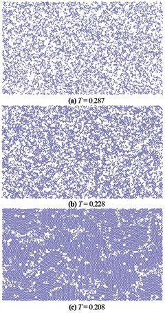
Figure 10. 2D visualization of the occurrence/growth of atoms with  in models obtained at the cooling rate of
  per MD step and at different temperatures.
Download figure:
Standard image High-resolution imageFinally, we stop here to discuss additionally the stability of 2D crystals in general, and some classical MD or MC simulations related to the formation of graphene, a real ideal 2D crystal. It is stated that in purely 2D crystals, thermal fluctuations would destroy a long range order at any finite temperature, this is called the Mermin-Wagner theorem (see for example, [40]). These fluctuations can be suppressed by anharmonic coupling between bending and stretching modes, i.e. a 2D membrane can exist but will exhibit strong height fluctuations [41–43]. Indeed, recent experiments and computer simulations confirm the existence of strong ripples in graphene [7, 44]. However, another possibility, consistent with the Mermin-Wagner theorem, has been proposed recently: 2D crystals can be stabilized by short-range distortions where the neighboring atoms are shifted in the third dimension in opposite directions [45]. Note that our 2D sheets with honeycomb structure eventually collapse leading to the formation of 3D atomic configurations if it is relaxed at a given temperature in 3D space. Fast collapse of our 2D honeycomb structures is due to a softness of the honeycomb interatomic potential compared to that of the more realistic many-body LCBOPII potential used for graphene in [7]. Note that all results shown and discussed in the present work have been obtained by MD simulations in a rigid 2D simulation cell. On the other hand, although one can find some MD or MC simulations related to the formation of graphene with realistic interatomic potentials [7, 10, 31, 46, 47], the atomic mechanism of the formation of graphene obtained by quenching from the melt has not been analyzed yet. On the other hand, detailed analysis of structural defects of 'a real graphene' obtained by quenching from the melt at various cooling rates has not been done yet. Therefore, our comprehensive MD simulations in this direction highlight the situation.
4. Conclusions
We have carried out MD simulations of the 'graphenization' of 2D simple momatomic liquids and some important conclusions can be drawn as follows:
- (i)We find the formation of amorphous and crystalline 2D materials with honeycomb structure from 2D simple supercooled monatomic liquids with honeycomb interatomic pair potential depending on the cooling rate used in simulations. The former exhibits a smooth change in structural and thermodynamic quantities like that commonly found for glass formation in 3D supercooled liquids, while the latter exhibits usual first-order behavior with a sudden change in various structural and thermodynamic properties of the system at the transition. The model with honeycomb pair interatomic potential is simple and it is relevant for further simulations in this direction in order to get new insights into the structural properties, including various defects and their dynamics, the atomic mechanism of phase transitions, etc. of real 2D materials such as graphene, silicene, germanene ... since these materials also have a honeycomb structure.
- (ii)The atomic mechanism of the formation of a 2D crystalline honeycomb structure from the liquid state can be described as follows: (i) Upon cooling from the melt, atoms involving 6-fold rings and/or atoms with
 occur locally and homogeneously throughout the system, at temperatures close to freezing their number grows fast with further cooling; (ii) Atoms involving 6-fold rings and/or atoms with have a tendency to form clusters of a hexagonal order, these clusters grow fast with decreasing temperature and then they merge into a single percolation cluster which spans throughout the system. Further cooling just enhances the atomic population of the percolation cluster to form a final rigid honeycomb configuration.
 - (iii)Our relatively large models exhibit polycrystalline structure, the grain boundaries of which consist of various types of structural defects including various types of vacancies, 5-fold and 7-fold rings, adatoms etc. Our finding gives deeper understanding of the structure of the grain boundaries of polycrystalline graphene or similar 2D materials in general.
- (iv)About 95% of rings in our crystalline honeycomb structure are 6-fold, indicating that 6-fold rings are indeed building blocks of the honeycomb structure. However, we find that ring distribution in the models is rather wide-ranging, from 3-fold to 13-fold, although the fraction of the rings larger than 9-fold is very small. Extra-large-member rings lead to the formation of vacancies of unusual shapes which have not been mentioned in the past. Rings with sizes other than 6-fold can be considered as structural defects and they may act as highly reactive sites in the honeycomb structure of 2D materials.
- (v)We find a large number of various types of vacancies, including multiple ones in the crystalline honeycomb structure. We also find 'unusual' defects—adatoms with a significant amount. These vacancies and defects are not artificial results, due to the 2D simulation setup, but should be the result of a 'synthesis' method. These vacancies and defects have not been previously reported yet. Moreover, the existence of adatoms graphene has been ignored, based on the speculation of their high formation energy in solid 2D materials. However, based on our MD simulations one can suggest that adatoms should exist in real 2D materials synthesized from the molten state and/or by the CVD since they can form initially in the liquid state prior to freezing and then frozen further upon cooling, i.e. requiring a much lower formation energy of the adatoms compared to those formed in the solid state.


Acknowledgments
This research is funded by the Vietnam National Foundation for Science and Technology Development (NAFOSTED) under Grant number 103.02–2012.17. The author thanks Mr Tran Phuoc Duy (a graduate student) for running calculations on LAMMPS.