
Abstract
The electronic and magnetic properties of the transition metal sesqui-oxides Cr2O3, Ti2O3, and Fe2O3 have been calculated using the screened exchange (sX) hybrid density functional. This functional is found to give a band structure, bandgap, and magnetic moment in better agreement with experiment than the local density approximation (LDA) or the LDA+U methods. Ti2O3 is found to be a spin-paired insulator with a bandgap of 0.22 eV in the Ti d orbitals. Cr2O3 in its anti-ferromagnetic phase is an intermediate charge transfer Mott–Hubbard insulator with an indirect bandgap of 3.31 eV. Fe2O3, with anti-ferromagnetic order, is found to be a wide bandgap charge transfer semiconductor with a 2.41 eV gap. Interestingly sX outperforms the HSE functional for the bandgaps of these oxides.
Export citation and abstract BibTeX RIS
1. Introduction
Transition metal oxides are an important class of functional materials (e.g. [1]). They also provide a useful test of electronic structure theories because of their localized d electrons [2–7]. NiO is frequently used as a test case for such theories. Here, we treat the corundum structure transition metal sesqui-oxides, Ti2O3, Fe2O3, and Cr2O3, which span the range from a narrow bandgap diamagnetic semiconductor to a wide bandgap anti-ferromagnetic insulator. The bandgap of Ti2O3 is small, about 0.1 eV, and it has been argued whether the small gap arises from Coulombic interactions or from Ti–Ti ion pairing [8]. α-Fe2O3, hematite, with an experimental bandgap of 2.2 eV [9] was identified as a charge transfer semiconductor [2]. Experimentally, from to photoemission spectra [10], Cr2O3 is considered to be intermediate between a charge transfer insulator and a Mott–Hubbard insulator.
Density functional theory (DFT) has been the standard method for calculating the electronic properties of solids. The most widely used functionals are the local spin-density approximation (LSDA) and the spin polarized generalized gradient approximation (GGA). However, both these functionals underestimate the bandgap for simple sp semiconductors and insulators due to the lack of self-interaction cancelation and incorrect description of exchange and correlation with respect to changes in particle number. This problem becomes more severe in systems with localized d or f open shells such as transition metal or lanthanide compounds. A local functional may give qualitatively the wrong electronic structure. For example, the LDA describes Ti2O3 as a metal [11, 12], rather than with a bandgap of 0.1 eV. GGA underestimates the experimental bandgap of Fe2O3 by 75%. LSDA gives a bandgap of Cr2O3 of 1.5 eV [13] compared to an experimental value of 3.2–3.4 eV [14].
One way to improve the LDA for d electron systems can be to include an on-site Coulomb repulsion leading to the LDA+U or GGA+U methods [3]. But the U parameter is often empirically found by fitting to experimental bandgaps. Even after the fitting process, the bandgap of Cr2O3 is 10–20% underestimated and the magnetic moment is significantly smaller in LDA+U and GGA+U than in experiment [15–17]. On the other hand, the Hartree–Fock (HF) method with exact exchange greatly overestimates the bandgaps of Ti2O3 and Cr2O3 [18–20].
A better method for improving on LDA can be to use hybrid density functionals. These functionals mix some part of the exact exchange from HF into the LDA or GGA potential [21]. This expression for the exchange interaction has self-interaction correction, and so they provide perhaps the best one-particle description of electronic structure, much better than LDA or GGA for non-metallic systems. A key advantage of hybrid functionals is that they are generalized Kohn–Sham functionals, so they can be used variationally to obtain total energies [21, 22] and for structural optimizations, as forces and stresses can be evaluated straightforwardly [23].
An example of a hybrid functional is the Heyd, Scuseria, Ernzerhof (HSE) functional. This separates the exchange energy into short-range and long-range parts and replaces some of the short-range part of LDA exchange with HF exchange [24]. HSE can give good values for the bandgaps and valence band widths of standard semiconductors [25] and it has also been applied to oxides [26, 27]. Formally, perturbation theory suggests that 0.25 of HF exchange should be mixed into the LDA functional. Sometimes, the fraction of HF exchange is treated as a parameter, but with a loss of its ab initio character. HSE gives the bandgap of Fe2O3 as 4.0 eV with 25% HF fraction [27], nearly twice as large as the experimental value. If 12% of HF exchange is used, this gives a bandgap of 1.95 eV, closer to experiment, but the magnetic moment is 15–20% too small [27]. Another hybrid functional, B3LYP, gives a bandgap of Cr2O3 which is close to the experimental value [28].
There are some methods beyond DFT which can be very accurate. One choice is the GW approximation [29]. The GW method based on LDA+U can give the correct bandgap for several simple transition metal and lanthanide oxides [4–7]. So far there are only a few reported GW band structure results for the corundum oxides [30].
Another method beyond LDA is dynamic mean field theory (DMFT), which includes the strong electron correlation in the calculation where electrons behave beyond the quasi-particle model [31–33]. DMFT with an empirical value of the Coulomb interaction can give the correct band structure for Ti2O3 [33].
Transition metal oxides provide some of the most interesting systems with metal–insulator transitions (MIT) such as Ti2O3, V2O3, VO2, and the manganites [33–35]. In some cases, the MIT depends on the local bond lengths. The difficulty of using GW or most DMFT implementations for geometric optimization means that they tend to be used for post-processing the electronic structure, given a certain atomic geometry, except in a few cases [36]. The benefit of hybrid functionals is that they offer the possibility to do structural optimization with a good single-particle electronic structure in a single shot, so they can capture the dependence of electronic structure on geometry even in difficult systems.
In this paper, we test one hybrid density functional, screened exchange (sX), on relatively simple transition metal oxides. sX is a parameter-free, self-consistent method that mixes a screened HF exchange into the local LDA functional [37–39]. It was previously shown that sX fixes the bandgap problem in sp-bonded semiconductors [38]. But it is unclear whether sX can correctly describe localized d electrons and their various magnetic orderings. The corundum structure transition metal oxides provide such a test. The band structure and magnetic properties of Ti2O3, Fe2O3, and Cr2O3 from sX are compared to experiments and to the results of other methods.
2. Computational methods
The screened exchanged functional contains parts of the HF exchange potential where the exchange correlation energy explicitly depends on the orbital and includes the non-local parts. The Schrödinger equation has a non-local part and a generalized Kohn–Sham scheme is used:
where Vloc(r) is the local part of the exchange correlation function and i labels the electron states. The long-range exchange term is then screened by a Thomas–Fermi exponential factor. The local part of the LDA is added in to ensure that the hybrid functional is correct at the homogeneous electron gas limit. The sX functional can be represented by
where kTF is the Thomas–Fermi screening vector, i,j label the electron bands, and k,q label the k points. The Thomas–Fermi screening vector is calculated from the s, p, d valence electron density [38] to be 2.37 Å−1, 2.46 Å−1, and 2.49 Å−1 for Ti2O3, Cr2O3, and Fe2O3, respectively.
The calculations were carried out in the CASTEP plane-wave pseudopotential code [40]. Norm-conserving pseudopotentials were generated by the OPIUM method [41] with LDA used for the exchange correlation. The pseudopotential parameters are summarized in table 1. The Brillouin zone integrations use a 4 × 4 × 4 Monkhorst–Pack grid [42]. The magnetic moments are calculated by the Mulliken model of atomic charge [43]. The band structure is calculated with the experimental value of lattice constants. A Monkhorst–Pack grid of 5 × 5 × 5 is used for calculating the density of states (DOS).
Table 1. Valence electron configurations and cutoff energies used for generating the norm-conserving pseudopotentials. All potentials are generated with the LDA approximation.
| Electron configuration | Cutoff energy (eV) | |
|---|---|---|
| Ti | 3d24s2 | 400 |
| Cr | 3d54s1 | 700 |
| Fe | 3d64s2 | 500 |
| O | 2s22p4 | 780 |
The three sesqui-oxides have the same crystal structure as that shown in figure 1. The primitive cell is rhombohedral (space group R3c) with two formula units. This can be regarded as a distortion of the cubic perovskite structure along the 〈111〉 direction. The transition metal atoms lie along the c-axis (the body diagonal). However, the metal atom positions can vary. The lattice constants for the ground state calculation are summarized in table 2. The Ti–Ti distance along the c axis is also listed for comparison. Each transition metal atom has six nearest O neighbors within a distorted octahedral configuration. The anti-ferromagnetic ordering occurs by alternating the spin direction along the body diagonal.

Figure 1. Crystal structure of the corundum structure. The transition metal atoms are label as gray while O is red. (a) The rhombohedral primitive cell. The lattice constants used for ground state calculation are defined in table 1. The transition metal distances are along the c axis. The spin structure in table 3 describes the spin states of Cr atoms in the body diagonal. (b) The hexagonal representation.
Download figure:
Standard imageTable 2. Lattice parameters used for ground state calculation.
| Lattice constant (Å) | Angle (deg) | |
|---|---|---|
| Ti2O3 | 5.431 | 56.583 |
| Cr2O3 | 5.390 | 55.130 |
| Fe2O3 | 5.419 | 55.364 |
3. Results and discussion
We first describe the semi-empirical ligand field and molecular orbital models that were previously used to describe the electronic structure in these oxides. The octahedral coordination of the transition metal atoms in the corundum structure splits the 3d state into t2g and eg orbitals. The transition metal atoms are in their 3+ ion state, leaving 1, 3, and 5 valence electrons on Ti, Cr, and Fe ions, respectively. In Ti2O3, the pair of Ti atoms on face-sharing octahedra can approach each other, so this trigonal distortion causes an additional splitting of eg–a1g bands. The Ti–Ti pairs form bonding and anti-bonding states. This Zandt–Honig–Goodenough model [44] predicts that there is a small bandgap between the a1g levels and the eg levels (figure 2). The simple ligand field models left the exact nature of the bandgaps in Fe2O3 or Cr2O3 unclear, either charge transfer or Mott–Hubbard.

Figure 2. The ligand field splitting of the 3d orbitals in Ti2O3.
Download figure:
Standard image3.1. Ti2O3
Although Ti2O3 has the same corundum structure as Cr2O3 and Fe2O3 its electronic structure is quite different. The ground state of Ti2O3 at low temperature is diamagnetic. Crystal field theory explains the small bandgap from the splitting of Ti d orbitals by a trigonal distortion of the neighboring oxygens and a Ti–Ti pairing.
The spin polarized sX functional is used to relax the structure and calculate the total energy, band structure and density of states. The structural relaxation results from PBE and sX are compared in table 3. The metal–metal distance along the c axis in Ti2O3 is much smaller than in Cr2O3 and Fe2O3. Both PBE and sX underestimate the Ti–Ti pair distance but sX gives better results. The error with respect to the experimental value has been reduced from over 6% in PBE to 3% in sX. The shorter Ti–Ti distance leads to a larger energy splitting of the bonding and anti-bonding states, which widens the energy bandgap.
Table 3. Metal–metal distances along the c axis as a ratio of the M–oxygen distance.
| M–M distance | Å | As ratio of M–O distance | ||||
|---|---|---|---|---|---|---|
| PBE | sX | Experiment | PBE | sX | Experiment | |
| Ti2O3 | 2.385 | 2.466 | 2.591 | 1.155 | 1.206 | 1.245 |
| Cr2O3 | 2.670 | 2.669 | 2.664 | 1.325 | 1.325 | 1.317 |
| Fe2O3 | 2.871 | 2.901 | 2.881 | 1.375 | 1.388 | 1.380 |
Figure 3 shows the sX band structure of Ti2O3 for the structure relaxed in sX. The resulting bandgap is found to be 0.55 eV, compared to 0.1 eV in experiment [8, 45]. If the smaller experimental Ti–Ti distance is used, the bandgap is 0.22 eV in sX. The electron states are found to be spin-paired along the Ti–Ti bond, as in the Zandt–Honig–Goodenough model [44]. The valence band maximum (VBM) lies between R and Γ and the conduction band minimum lies at the A point (0.5, 0.5, 0). The direct bandgap at Γ is 0.70 eV. Local functionals like LDA and GGA both give a metallic band structure with no bandgap [11, 12]. The HF method overestimates the bandgap by over 10 eV [16]. The only comparable computational result to ours is a bandgap of about 0.1 eV from the LDA+DMFT method with an empirical on-site repulsion [31]. The ability of sX to give an reasonable bandgap, magnetic structure and metal–metal bond length for Ti2O3 suggests that sX can be useful for studying more complex MIT systems.

Figure 3. (a) Spin polarized band structure of Ti2O3 and (b) close-up of the bands near the bandgap, for the experimental atomic structure.
Download figure:
Standard imageThe total and partial DOS (PDOS) from sX are plotted in figure 4. A small Gaussian smoothing of 0.02 eV of the DOS is used in order to identify the small bandgap. The PDOS shows that the valence band and conduction band are both formed by Ti 3d orbitals. The O p orbitals lie well below the Fermi level. The residual states near EF on the O atoms are due to the error in the Mulliken model when calculating the PDOS and are neglected. The DOS and PDOS are in good agreement with the Zandt–Honig–Goodenough ligand field model [44] and angle resolved photoemission data [46]. The valence band width of the Ti 3d orbitals is 1.6 eV and that of the O p orbitals is about 4.5 eV below EF, consistent with experimental values of 1.5 and 4.0 eV [46]. There is another small gap in the conduction band, about 2.5 eV above EF. This is due to the splitting of a1g anti-bonding states and the eg states. LDA gave a zero bandgap but the relative position of the d states is correct.
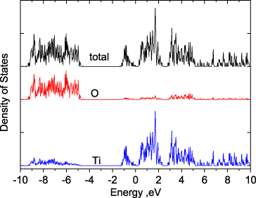
Figure 4. Total and partial density of states of Ti2O3.
Download figure:
Standard imageThe charge density of the highest occupied a1g band is plotted in figure 5. Only the Ti atoms along the c axis and their O neighbors are plotted to show the relative position. The state has a rather pure a1g 3z2 − r2 character. The density in real space has similar symmetry and shape to the a1g orbital in other transition metals from LDA+U [47] and the exact exchange calculation [26]. Moreover, the bonding state due to the close contact of neighboring Ti atoms is clearly seen in real space. The electron density of each Ti atom overlaps more as their separation decreases. The state is centered on the Ti atoms and there is no charge density around O atoms, which confirms that the bandgap is a pure Ti d state.

Figure 5. The orbital density of the a1g orbitals Ti2O3 (left) and Cr2O3 (right), showing the bonding state in Ti2O3 and anti-ferromagnetic spin ordering in Cr2O3.
Download figure:
Standard imageFigure 6 shows the total valence charge density for Ti2O3 (along with that for Cr2O3 and Fe2O3). The valence charge is highly localized around the O ion in Ti2O3 and note that it reduces in the Cr and Fe oxides as the ionicity decreases along this series.

Figure 6. Valence charge densities of Ti2O3, Cr2O3, and Fe2O3, showing ionicity decreasing towards Fe2O3.
Download figure:
Standard image3.2. Cr2O3
The electronic states of Cr2O3 with different magnetic ordering have been calculated: three anti-ferromagnetic (AFM) phases with different magnetic orderings, a ferromagnetic (FM) phase, and a paramagnetic (PM) phase. The AFM and FM phases are calculated with the spin polarized sX while the PM phase is calculated with non-spin-polarized sX. The magnetic order and the total energy are summarized in table 4. The G-type AFM phase is the ground state at 0 K, as seen in both experiments and simulation [13]. The energy differences between various magnetic phases are significantly larger, which is possibly due to the experimental lattice constants used for the calculation. In the LSDA calculation, the lattice constant changes by about 1–5% for the FM and PM phases compared with the AFM phase [13]. The energy differences between AFM phases with different magnetic ordering are much smaller. The geometry relaxation shows some improvement. The error of the Cr–Cr distance has been reduced by 30%.
Table 4. Total energy per Cr atom of different magnetic phases of Cr2O3 with respect to the ground state.
| G-type AFM | AFM II | AFM III | FM | PM | |
|---|---|---|---|---|---|
| Magnetic ordering | +−+− | ++−− | +−−+ | ++++ | None |
| Energy difference (eV) | 0 | 0.04 | 0.09 | 2.11 | 7.32 |
Figure 7 shows the calculated spin polarized band structure of Cr2O3. The total and partial density of states are plotted in figure 8. The VBM is set to 0 eV. Cr2O3 has an indirect bandgap of 3.31 eV, compared to an experimental gap of ∼3.4 eV. The VBM is between the X and Γ points and the conduction band minimum is at A (0.5, 0.5, 0). The direct bandgap at Γ is 3.9 eV. From the PDOS, we can clearly see the hybridization of the O p and Cr d states in both the VBM and CBM. The PDOSs of Cr and O agree quite well with the x-ray photoemission spectra [10, 49, 50].

Figure 7. Band structure of anti-ferromagnetic Cr2O3.
Download figure:
Standard image
Figure 8. (a) Total and partial DOS of anti-ferromagnetic Cr2O3, including spin up and spin down on one of the Cr atoms. (b) Total DOS of paramagnetic Cr2O3 using the pair-cluster model.
Download figure:
Standard imageThe calculated magnetic moment of Cr ion in sX is 3.52 μB, which is significantly better than other methods but is still 10% less than the experimental value (table 6). The Cr ion is considered to be completely ionized in the experiments, while in fact O p and Cr d orbitals are hybridized both in the valence band and the conduction band. The O 2p hybridization will decrease the magnetic moment of Cr atoms [15]. The local atomic orbitals basis set of the Mulliken model [43] could further decrease the calculated magnetic moment slightly.
Table 5 compares the calculated bandgaps of Cr2O3 for different exchange functionals and experiment. sX gives a bandgap of 3.31 eV, in good agreement with the optical value of 3.3 eV [13]. Photoemission experiments give a slightly larger bandgap of 3.4–3.5 eV [49]. The HF method overestimates the bandgap [18] while the LDA/GGA underestimates it [13], as expected. The bandgaps from LDA+U/GGA+U show significant improvement over LDA/GGA, but the error is still ∼20% [15]. This is perhaps due to the mixed character of both conduction and valence band edges. Interestingly, the B3LYP hybrid functional gives a bandgap of 3.4 eV [28], close to experiment and sX, whereas HSE gives a bandgap of 4.4 eV [46], much greater than experiment.
Table 5. Experimental and calculated bandgaps (eV).
| Bandgap (eV) | HF | LDA/GGA | DFT+U | HSE | B3LYP | sX | G0W0@LDA+U | Expt. |
|---|---|---|---|---|---|---|---|---|
| Ti2O3 | 14.1 [18] | 0 [11, 12] | — | — | 0.22 | 0.1 [6, 45] | ||
| Cr2O3 | 15 [19] | 1.5 [13] | 2.9 [15] | 4.4 [48] | 3.4 [26] | 3.31 | 3.4 [14] | |
| Fe2O3 | 15.7 [20] | 0.3–0.5 [16, 51] | 2.9 [16] | 2.56 [27] | 2.41 | 2.8 [30] | 2.2 [7] |
Both LSDA and GGA predicted a small bandgap of 1.2–1.5 eV. Because there is a small gap between O p states and Cr d states and the valence band edge is completely composed of Cr 3d states, the authors [13, 17] suggested that Cr2O3 was a typical Mott–Hubbard insulator. The results from GGA+U and LDA+U are inconsistent. GGA+U predicts a hybridization of O 2p and Cr 3d states in the valence band edge, identifying Cr2O3 as an intermediate charge transfer (CT)–Mott–Hubbard (MH) insulator [16]. On the other hand, LDA+U gives a gap in the valence band separating the Cr and O orbitals, indicating a typical MH insulator [17]. sX finds that the O 2p and Cr 3d orbitals strongly hybridize throughout the valence band. There is a small gap of 1.5 eV below the bandgap, but both O 2p and Cr 3d contribute to the valence band edge, so it is concluded that Cr2O3 is a mixed CT–MH insulator.
The electronic structure of the paramagnetic phase was calculated in sX using the pair-cluster model of Shi et al [17], in which Cr pairs along Oz remain AF ordered but spins between pairs are randomized. It is found to be an insulator with a bandgap of order 3.4 eV from the DOS in figure 8(b), slightly less that in the AFM case. Clearly, the pairing effect dominates.
3.3. Fe2O3
The ground state of Fe2O3 is an AFM phase with a G-type ordering along the body diagonal. Different magnetic ordering including the G-type AFM (+−+−) and A-type AFM (++−−) states have been found with the spin polarized sX functional using the experimental observed lattice constants. The G-type order has been confirmed as the ground state.
Figure 9 shows the spin polarized band structure of hematite for the sX functional. We find that Fe2O3 has an indirect bandgap of 2.41 eV, compared with an experimental value of 2.2 eV [9]. The VBM is between R and the Γ point and the conduction band minimum is at M. The direct bandgap at Γ is 2.90 eV, slightly larger than the experimental value of 2.7 eV [7]. The band structure is similar to that from HSE [27]. GGA gives a direct bandgap of 1.17 eV and an indirect bandgap of 0.67 eV [16, 49], while HF overestimates both gaps as 15.6 and 15.7 eV [19]. The LDA/GGA+U method could give a better description but its U and J terms are fitted to the bandgap and magnetic moments [16]. It has been pointed out that these empirical values, while giving the correct results compared with measurements, might not give the correct underlying physical picture [10]. The HSE hybrid functional has been successfully applied to many semiconductors [25]. However, the HSE06 functional with a 25% HF potential gives 3.41 eV and 4.02 eV for the indirect and direct bandgaps, respectively [27], 70% larger than experiment. In order to decrease the bandgap, the fraction of HF potential was reduced. HSE with 12% HF potential gives 1.95 and 2.54 eV for the bandgaps [27]. The sX functional predicts the best band structure without any fitting to experimental measurements.

Figure 9. Band structure of anti-ferromagnetic Fe2O3.
Download figure:
Standard imageFigure 10 shows the sX total and partial DOS of Fe2O3. The PDOS of Fe is from just one Fe atom in the unit cell, to distinguish the spin-up and spin-down difference. The shape of the sX PDOS agrees well with the photoemission and inverse photoemission spectra [49, 52, 53]. It is clear that the calculated VBM is purely from oxygen 2p states, while the Fe 3d states dominate the CBM, which confirms that Fe2O3 is a charge transfer semiconductor. GGA predicts the bandgap to be Fe d–d type rather than an O 2p–Fe 3d charge transfer type [51]. HF does give the correct p–d charge transfer bandgap, but the gap value is grossly in error. The results from the LDA+U model are not so consistent. Different U values were used to generate the experimental bandgap [16, 51]. The sX PDOS for O and Fe are similar to a GGA+U spectrum with a large U value [16].

Figure 10. Total and partial density of states, including spin up and spin down on one of the Fe atoms.
Download figure:
Standard imageThe magnetic moment of Fe is calculated to be 4.39 μB compared to an experimental value of 4.67 μB [54] (table 6). In contrast, LDA/GGA [51] underestimates the magnetic moment by 30–40%. In the HF method a compromise between parameters leads to 4.0 μB [19]. For the HSE functional, the HF fraction has little effect on the magnetic moment—HF fractions of both 12% and 25% gives the same value [27].
4. Conclusion
The sX hybrid functional is used to calculate the electronic and magnetic properties of several corundum structure transition metal oxides. The results are compared to other density functional methods. sX gives accurate bandgaps, orbital types and magnetic moments of each oxide, and gives band widths consistent with photoemission. Ti2O3 is found to be spin-paired with a small bandgap of 0.2 eV due to a bonding–anti-bonding splitting of its 3d a1g states. Cr2O3 is found to be an intermediate CT–MH insulator with an indirect bandgap of 3.31 eV, close to experiment, and a calculated magnetic moment of 3.52 μB compared to an experimental value of 3.8 μB. Fe2O3 is a typical charge transfer semiconductor with a bandgap of 2.41 eV and anti-ferromagnetic order. The magnetic moment of the Fe atom is 4.39 μB compared to an experimental value of 4.64 μB. Interestingly sX gives a bandgap and magnetic moment closer to experiment than the HSE functional for Fe2O3. Overall, sX is an accurate and efficient functional to describe the one-electron states and magnetic structures in these systems with localized 3d states. It is likely be useful as a means for calculating geometry-dependent electronic structures for more complex systems with metal–insulator transitions.