
Abstract
The effect of ionic solute on a near-critical binary aqueous mixture confined between charged walls with different adsorption preferences is considered within a simple density functional theory. For the near-critical system containing small amounts of ions, a Landau-type functional is derived on the basis of the assumption that the correlation, ξ, and the Debye screening length, κ−1, are both much larger than the molecular size. The corresponding approximate Euler–Lagrange equations are solved analytically for ions insoluble in the organic solvent. A nontrivial concentration profile of the solvent is found near the charged hydrophobic wall as a result of the competition between the short-range attraction of the organic solvent and the electrostatic attraction of the hydrated ions. An excess of water may be present near the hydrophobic surface for some range of the surface charge and ξκ. As a result, the effective potential between the hydrophilic and the hydrophobic surface can be repulsive far from the critical point, then attractive and again repulsive when the critical temperature is approached, in agreement with a recent experiment (Nellen et al 2011 Soft Matter 7 5360).
Export citation and abstract BibTeX RIS
For more information on this article, see LabTalk.
A near-critical binary mixture confined in a slit induces effective attraction or repulsion between the confining walls if the adsorption preferences of the two walls are the same or opposite respectively [1–3]. The range of this so called thermodynamic Casimir force is of the order of the bulk correlation length ξ. Parallel walls covered with electric charges of the same sign repel each other. One could thus expect stronger repulsion between like charged walls with opposite adsorption preferences confining the near-critical binary mixture. In striking contrast to the above expectation, in the recent experiments of [4] strong attraction was observed between a charged hydrophobic colloid particle and a charged hydrophilic substrate for some range of temperatures and concentrations of a hydrophilic salt added to the solution. The effective interactions between the colloid particles separated by distances much smaller than their radii are similar to the interactions between planar surfaces. The possibility of changing these interactions from attraction to repulsion through minute changes of temperature or salinity opens possibilities for designing and controlling reversible structural changes, in particular, aggregation or adsorption. It is thus important to understand the mutual influence of the critical adsorption and the distribution of ions that leads to the attraction between the walls instead of the expected repulsion. We address this issue in this communication.
We consider a mixture of water and organic liquid, containing hydrophilic ions in a slit with selective, charged walls of the area A→∞, separated by the distance L ≫ 1 (figure 1). We choose the average diameter of the molecules, a≡1, as the length unit and all the corresponding functions are dimensionless. The grand thermodynamic potential of the system can be written in terms of the local dimensionless densities ρi(r), where i = 1–4 for water, oil, and + and − ions respectively, in the form [5]
where p is the bulk pressure, the integration is over the system volume V = AL, periodic boundary conditions are imposed in the directions parallel to the walls, and S, Uel, T and μi are the entropy, electrostatic energy, temperature and chemical potential of the ith species respectively. Vij and gij are the van der Waals (vdW) interactions and the pair correlations between the corresponding components respectively, and the summation convention for repeated indices is assumed in the whole communication.  is the sum of the direct wall–fluid potentials acting on the component i. Finally,

is the excess grand potential per surface area, γn is the surface tension at the nth wall (n = 0,L), and the effective potential Ψ(L) is the subject of our study. Because of the translational symmetry in the parallel directions, the densities depend only on the distance from the left wall, z. We make the standard approximation
and the standard assumption [7]
where the electrostatic potential ψ satisfies the Poisson equation,
e is the elementary charge,  is the dielectric constant of the solvent, σ(n) is the dimensionless surface charge density at the nth wall, and

is the dimensionless charge density. Compressibility of the liquid can be neglected, and we assume that  . We choose ϕ, the solvent concentration s = ρ1−ρ2, and the density of ions ρc = ρ3 + ρ4 as the three independent variables. Bulk equilibrium densities for given T and μi correspond to the minimum of −pAL, and are denoted by
  and
and  . In equilibrium, ϕ(z) and the deviations from the bulk values

correspond to the minimum of ![${\omega }_{\mathrm{ex}}[{\vartheta }_{1},{\vartheta }_{2},\phi ]=(\Omega [{\vartheta }_{1}+\bar {s},{\vartheta }_{2}+{\bar {\rho }}_{\mathrm{c}},\phi ]-\Omega [\bar {s},{\bar {\rho }}_{\mathrm{c}},0])/A$](https://content.cld.iop.org/journals/0953-8984/23/41/412101/revision1/cm393795ieqn50.gif) with
with  and
and  fixed. We choose for
  and
and  the values corresponding to the critical point.
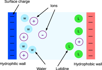
Figure 1. Model system consisting of water, organic liquid (for example lutidine) and ions between negatively charged hydrophilic (dark, blue) and hydrophobic (light, red) walls.
Download figure:
Standard imageCommon salts are soluble in water and insoluble in organic solvents. We thus assume that the difference in chemical nature of the anion and the cation is negligible, and postulate the same vdW interactions, Vi,3 = Vi,4. From equation (1) it easily follows that the vdW contribution to the internal energy expressed in terms of the new variables is independent of ϕ when Vi,3 = Vi,4 [6]. Because Uel is independent of ϑi (see equation (4)), in this approximation the vdW and the electrostatic contributions to the internal energy are decoupled. The coupling is present in the entropic part. The excess entropy, ![${s}_{\mathrm{ex}}[{\vartheta }_{1},{\vartheta }_{2},\phi ]=(S[{\vartheta }_{1}+\bar {s},{\vartheta }_{2}+{\bar {\rho }}_{\mathrm{c}},\phi ]-S[\bar {s},{\bar {\rho }}_{\mathrm{c}},0])/A$](https://content.cld.iop.org/journals/0953-8984/23/41/412101/revision1/cm393795ieqn60.gif) , can be Taylor expanded in terms of ϑi(z) and ϕ(z). For a near-critical mixture with small amount of ions the expansion can be truncated, because ϑi(z) and ϕ(z) are small (except at microscopic distances from the surfaces). Using equation (3) one can verify that the excess entropy contains no terms proportional to
, can be Taylor expanded in terms of ϑi(z) and ϕ(z). For a near-critical mixture with small amount of ions the expansion can be truncated, because ϑi(z) and ϕ(z) are small (except at microscopic distances from the surfaces). Using equation (3) one can verify that the excess entropy contains no terms proportional to  , and the lowest-order mixed term is ϕ2ϑ2. Thus, the excess grand potential can be split in two leading-order terms and the correction ΔL:

From the minimum condition for ωex it follows that the linear terms vanish, and the dominant terms in equation (8) are quadratic in the fields ϑi(z) and ϕ(z). The second term on the RHS of equation (8) has the form

Equations (9), (4) and (5) agree with the Debye–Huckel (DH) theory for the excess grand potential of ions in a homogeneous solvent confined in a slit with charged walls. The first term in equation (8) is equal to the excess grand potential per unit area for one kind of neutral solute in a two-component solvent, where the excess concentration of the solvent and the excess solute density are denoted by ϑ1 and ϑ2 respectively and the total density is fixed. This is because we assumed no difference between the vdW interactions of the anion and the cation—when uncharged, they represent the same species in this theory. Close to the critical temperature Tc the fields ϑi(z) vary on the length scale ξ∝|(T−Tc)/Tc|−ν ≫ 1 with ν≈0.63, and the standard coarse-graining procedures leading to the Landau functional can be applied [8]. Our coarse-graining of the first term in equation (1) (expressed in terms of the new variables) is based on the Taylor expansion of ϑi(z') about z' = z. The excess grand potential is expressed in terms of the fields ϑi and their derivatives, and in terms of the appropriate moments of the vdW interaction potentials,
where
 and
and  . −Jij(r) represents the vdW interactions for ϑi and ϑj, and can be obtained from the vdW contribution to equation (1) with the densities expressed in terms of the new variables. We shall assume that the interaction ranges ζij defined by
  are all ζij≈1, and characterize the system with three interaction parameters,
  (for the length unit a≡1). Finally, hi(n) is the surface field describing interactions with the nth wall. The remaining surface terms result from the compensation for the interactions with the missing fluid neighbors at the wall. These interactions are included in the bulk term, but should be absent if the wall is present. In [6] the same functional was obtained from a lattice model for the four-component mixture. When the mixture phase separates, both the solvent concentration and the density of solute are different in the coexisting phases, because the solute is soluble only in water. Thus, LC must depend on both ϑ1 and ϑ2. The critical order parameter is the eigenvector of
  corresponding to the eigenvalue vanishing for T = Tc.
In equations (10) and (9) the terms proportional to kBT represent the leading-order contributions to the excess entropy per surface area. The next-to-leading-order contribution has the form
and results from the fact that there are more ways of introducing a local difference in the concentrations of the anions and the cations, ϕ(z), in the regions where there are more ions (ϑ2(z)>0) than in the regions where there are fewer ions (ϑ2(z)>0).
The Euler–Lagrange (EL) equations for the functional equations (8)–(12), with the higher-order terms defined in equations (10), (9) and (12) neglected, take the forms


The charge-neutrality condition,  , is imposed on ϕ, and the boundary conditions for ϑi are
In the above,  , where (J−1)ik is the (i,k)th element of the matrix inverse to the matrix Jij [6]. The remaining parameters are
  , and Hi(n)=−(J−1)ijhj(n). For a hydrophilic (hydrophobic) wall, H1 < 0 (H1 > 0).
When ΔL in equation (8) is neglected, the Casimir and the electrostatic potentials are independent contributions to ωex, and the EL equations are linear and decoupled (the second terms on the RHS of equations (13) and (14) are absent). In a semi-infinite system the solutions of the linearized EL equations (14) and (13) are


where Ai and Ci depend linearly on Hi. The superscript (1) refers to the solutions of the linearized EL equations. In the critical region, ξ→∞ and λ2 ≫ 1/ξ; therefore the second term on the RHS of equation (17) can be neglected. In the slit, the equilibrium fields ϕ(1)(z) and  also contain terms ∝exp(−κ(L−z)) and ∝exp(−(L−z)/ξ) respectively (and the amplitudes are modified). The effective potential Ψ(L) is obtained by subtracting the L-independent part from ωex calculated for the equilibrium profiles. Neglecting ΔL in equation (8) we obtain Ψ(L)=ΨDH(L)+ΨC(L) with ΨDH(L)∝exp(−κL) and ΨC(L)∝exp(−L/ξ).
The nonlinear terms in the EL equations (13) and (14) can be neglected when their magnitudes are much smaller than the magnitudes of the linear terms at the relevant length scales. The nonlinear contributions to equations (13) and (14) can be estimated by examining ϕ(1)2(z) and  for z = ξ and z = κ−1 respectively. This is because the linear terms in equations (13) and (14) decay on the length scales ξ and κ−1 respectively. From equations (16) and (17) we obtain ϕ(1)(ξ)∝exp(−ξκ) and
  . Thus, the magnitudes of the correction terms depend crucially on the ratio between the correlation and the screening length, ξκ. When ξκ→∞, then ϕ(1)(ξ)→0 and
  ; therefore we may consider the linearized equation (13), and treat equation (14) perturbatively. This case was considered in [6] for a semi-infinite system, and in [10] for a slit. On the other hand, for ξκ→0 we have ϕ(1)(ξ)=O(1) and
  ; therefore the linearized equation (14) can be considered. As a consequence, ϕ2 in equation (13) can be approximated by ϕ(1)2. In this approximation equation (13) takes the form of a linear inhomogeneous equation. We assume that this approximation is reasonable as long as ξκ < 1, and the magnitudes of σ2 and Ai are comparable.
In the experiments showing unusual dependence of the effective potential Ψ(L) on T, and consequently on ξκ, the relevant length ratio was ξκ < 1 [4]; therefore in this work we assume that ϕ = ϕ(1). Equation (13) with ϕ approximated by ϕ(1) can be easily solved analytically. The excess concentration of the solvent in the semi-infinite geometry takes the form

where  , B* depends on the vdW interactions and

The excess solvent concentration at the distance z from the hydrophobic surface with weak and strong surface charge is shown in figure 2 for a few values of ξκ ≤ 1 (note that in the figure captions the length unit a is re-introduced). In all the cases we observe an excess of organic liquid close to the surface. In some cases, however, ϑ1(z) is non-monotonic and changes sign for z0∼ξ. An excess of water appears at the distances z > z0 from the surface for all values of ξκ ≤ 1 in the case of strong surface charges. For weak surface charges an excess of water appears only for ξκ < y0(σ); for ξκ > y0(σ) a monotonic decay of |ϑ1(z)| occurs, as in the uncharged system. Thus, the presence of the surface charge can change a (weakly) hydrophobic surface to an effectively hydrophilic one if we pay attention to the concentration of water at sufficiently large distances from the wall, z∼ξ. A change of the adsorption preferences caused by increased surface charge was observed experimentally [3, 11]. We emphasize that the change of the adsorption preference for small or moderate surface charges is present only sufficiently far from the critical point.
The above properties can be understood by examining equation (18) for the hydrophobic surface (A1 < 0). For simplicity we neglect f1(κ,ξ) (f1(κ,κξ)→0 for ξ→∞ and κ→0, i.e. for T→Tc and  ), and assume ξκ > 0.5. For ξκ > 0.5 the second term in equation (18) decays faster, and at the length scale ξ the excess of water is found when the prefactor of the first term is positive. From equations (18) and (19) we can conclude that for T→Tc (i.e. ξκ→∞) the excess of water occurs (i.e. ϑ1(ξ)>0) when
  , which leads to the condition for the surface charge σ2 > 4|A1|/B1. When σ2 < 4|A1|/B1, an excess of organic liquid occurs (i.e. ϑ1(ξ)<0) for T→Tc. Since σ2B1f(ξκ) increases substantially when ξκ decreases (see equation (19)), the prefactor of the first term in equation (18), A1 + σ2B1f(ξκ), changes sign for ξκ = y0. Thus, for σ2 < 4|A1|/B1 a crossover from the excess of the organic liquid for ξκ > y0 (close to Tc) to the excess of water for ξκ < y0 (far from Tc) occurs for sufficiently large distances from the hydrophobic surface, z∼ξ.

Figure 2. The excess solvent concentration ϑ1(z) at the distance z from the charged hydrophobic surface for different values of ξκ with κ = 0.1a−1, where a is the molecular diameter. The dimensionless surface charge density (equation (4)) is (a) σ = 0.048/a2 and (b) σ = 0.092/a2, and in equations (18)–(20) A1 = −0.22a−3, B* = 0.54(kBTca2)−1, (J−1)1,2/B* = −12.52 and  . For a = 1 nm (the approximate size of the lutidine molecule),
  . z and ϑ1 are in units of a and a−3 respectively and ϑ1(z)>0 for an excess of water.
Download figure:
Standard imageThe physics behind such behavior is quite simple. The charged wall with no adsorption preference attracts ions. The ions insoluble in the organic liquid attract in turn water molecules to this wall. The excess number density of the hydrated ions (and thus the excess of water) appears in the layer of thickness ∼(2κ)−1 [7, 9] and depends on the surface charge. The charge-neutral, hydrophobic surface attracts organic molecules. An excess of organic liquid is found in the layer of thickness ∼ξ, and depends on the hydrophobicity of the surface. Competition between the excess of organic liquid and the excess of water near the surface which is both hydrophobic and charged depends on ξκ, on the surface charge and on the hydrophobicity of the wall, and leads to the nontrivial concentration profiles.
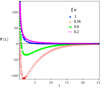
Figure 3. The effective potential per unit surface area between the charged hydrophilic and hydrophobic surfaces for the model system with  , for κ = 0.1a−1 and different values of ξκ shown in the inset. The surface fields (equation (15)) are H1(0)=−0.003a−3,H1(L)=0.002a−3,H2(0)=−H2(L)=−0.5a−3,
  ,
,  and the dimensionless surface charge density (equation (4)) is σ0 = σL = 0.065/a2. Ψ is in units of
  , and L is in units of a, where a is the molecular diameter (a≈1 nm for lutidine).
Download figure:
Standard imageThe Casimir potential between the walls results from the change of the concentration near the first wall caused by the presence of the second wall. Let us consider the vicinity of the hydrophilic wall when the weakly hydrophobic wall is present at the distance L∼ξ. The uncharged hydrophobic wall leads to depletion of water, but as discussed above and shown in figure 2, in the presence of the surface charge the hydrophilic ions can lead to the opposite effect. Thus, for the range of temperatures corresponding to the change of the adsorption preference of the weakly hydrophobic surface, the Casimir potential can be attractive. For a not too large surface charge it could overcome the electrostatic repulsion. We calculated Ψ(L) from equations (8)–(12) by inserting the solutions of equation (13) and linearized equation (14) with the boundary conditions given in equation (15). The result is shown in figure 3 for a particular model system. Indeed, the potential is repulsive far from the critical point because the electrostatic repulsion dominates, and becomes attractive and again repulsive when the critical temperature is approached.
The above theory is derived from the microscopic statistical mechanical description by a systematic coarse-graining procedure. We neglected any difference in chemical nature of the cation and the anion. The coupling between the excess concentration of the solvent, ϑ1(z), and the charge density, ϕ(z), results first from the coupling between ϑ1(z) and ϑ2(z) in equation (10), originating from the large difference in solubility of the hydrophilic ions in the two components of the solvent, and next from the coupling between ϑ2(z) and ϕ(z) of the entropic origin (see equation (12)). Very recently, similar behavior of Ψ(L) was obtained in [12]. The change of the adsorption preference in [12] results from different solubilities of the anion and the cation in water. Further studies are necessary to verify which mechanism plays the key role for the experimental results reported in [4].
Acknowledgment
We gratefully acknowledge discussions with A Maciolek, U Nellen, S Dietrich and C Bechinger. FP would like to thank Professor Dietrich and his group for hospitality during her stay at the MPI in Stuttgart. A part of this work was realized within the International PhD Projects Programme of the Foundation for Polish Science, cofinanced from European Regional Development Fund within the Innovative Economy Operational Programme 'Grants for innovation'. Partial support by the Polish Ministry of Science and Higher Education, Grant No NN 202 006034, is also acknowledged.