

Abstract
Four numerical codes are employed to investigate the dynamics of scrape-off layer filaments in tokamak relevant conditions. Experimental measurements were taken in the MAST device using visual camera imaging, which allows the evaluation of the perpendicular size and velocity of the filaments, as well as the combination of density and temperature associated with the perturbation. A new algorithm based on the light emission integrated along the field lines associated with the position of the filament is developed to ensure that it is properly detected and tracked. The filaments are found to have velocities of the order of  , a perpendicular diameter of around 2–3 cm and a density amplitude 2–3.5 times the background plasma. 3D and 2D numerical codes (the STORM module of BOUT++, GBS, HESEL and TOKAM3X) are used to reproduce the motion of the observed filaments with the purpose of validating the codes and of better understanding the experimental data. Good agreement is found between the 3D codes. The seeded filament simulations are also able to reproduce the dynamics observed in experiments with accuracy up to the experimental errorbar levels. In addition, the numerical results showed that filaments characterised by similar size and light emission intensity can have quite different dynamics if the pressure perturbation is distributed differently between density and temperature components. As an additional benefit, several observations on the dynamics of the filaments in the presence of evolving temperature fields were made and led to a better understanding of the behaviour of these coherent structures.
Export citation and abstract BibTeX RIS
1. Introduction
One of the biggest challenges in magnetic confinement fusion is to ensure compatibility between high fusion power and protection of the plasma facing components [1]. A problematic aspect related to this is the increase in the particle transport towards the wall (see e.g. [2, 3]), which can potentially enhance erosion and shorten the lifetime of the machine. Turbulent particle transport is largely due to coherent filamentary structures that propagate very far away from the last closed flux surface [4, 5]. In these fluctuations a significant fraction of the ion energy can be retained [6], thus potentially leading to a significant intermittent load on the wall materials.
Filaments, or blobs as they are sometimes called, were observed experimentally in both linear and toroidal machines and are present in L-mode and in H-mode, both during and between ELMs [7–11]. These transient events play a central role in determining the SOL profiles as they form the building blocks of anomalous transport [12]. To extrapolate present day experimental results to DEMO with sufficient confidence, predictive capability, based on first principle insight, must be obtained through development and validation of theoretical models.
We describe here the first systematic benchmark and validation of numerical codes and of the models they implement against experimental measurements of filamentary dynamics in the SOL of a tokamak device, the mega-ampere spherical tokamak (MAST). Our paper is an ideal extension to tokamak geometry of the work performed in [13], which investigated filaments in TORPEX [14, 15], a device characterised by a simple magnetized toroidal configuration. Our investigation is performed in a typical MAST double-null L-mode plasma, in conditions of collisionality that allow a fluid treatment of the equations in the open field lines region. The plasma conditions are quite different in MAST and in TORPEX, with the former having a characteristic SOL density three orders of magnitude higher and a temperature one order of magnitude higher. Also the external magnetic fields are dissimilar, with TORPEX values below 0.1 T on axis and MAST around 0.5 T. The experimental measurements in this work were mostly performed with visual camera imaging, which allows capturing several features of the filaments at time scales relevant for their dynamics (in contrast, [13] used Langmuir probes). While the experimental data in our work were obtained with newly developed techniques, the numerical tools used in both analysis are the same four SOL turbulence codes: the STORM module [16, 17] of BOUT++ [18], GBS [19], HESEL [20, 21] and TOKAM3X [22]. Note, however, that STORM has now implemented new features to better capture the experimental results, while here both GBS and HESEL employed a variety of approaches, beyond the ones used in [13].
Another element of novelty of our work is the direct comparison between numerical codes and individual filaments. In [13], the measurements were obtained using conditional averaging over several experimental realisations, thus providing 'statistical' rather than actual filaments. In addition, in our work we investigated isolated filaments in order to allow seeded filament simulations. This can be seen to complement a previous comparison between 2D simulations and experimental measurements in MAST aimed at understanding turbulence statistics [23].
2. Experimental observations
In this section, we describe the experimental data that the codes aimed at reproducing. In particular, we give an overview of the conditions in which the filaments were measured, we discuss the technique used to detect and track the motion of the filaments and finally we summarise the results of the experimental analysis.
2.1. Experimental conditions
We analysed a single MAST discharge (#29852), from which we extracted two well diagnosed filaments, selected on the basis of the quality of their measurements. The selection criteria were the persistence of the filament in multiple frames ( 4), its toroidal position (around ∼180 deg), to favour better resolved foreground perturbations and the separation from other filaments. The latter requirement was imposed to simplify the detection and tracking and to be consistent with the seeded filament approach of the simulations. It is worth noticing that we do not expect the toroidal location to affect the filament dynamics due to axisymmetry. In this work, we focus on two filaments of different size and amplitude, which in the following are referred to as filament 1 and filament 2.
The main features of the discharge investigated are graphically summarised in figure 1. Note that the nominal toroidal magnetic field is  T (at R = 0.66 m), which decreases to 0.19 T at the outer midplane separatrix. The poloidal magnetic field in the same location is
  T, which would give a total magnetic field of
  T, less than 20
 larger than BT. The discharge was a double null L-mode with
  MW of Ohmic and 1.7 MW of NBI heating (turned on at t = 0.05 s and kept on until termination) and with a plasma current
  MA. The plasma current flowed in the direction of positive toroidal angle (i.e. counter-clockwise), while the confining magnetic field was counter-current. Small sawtooth oscillations were present during the discharge, with a period of ∼8 m s, but the analysis of the filaments was performed during quiescent periods, far from crashes. In the plasma current flat top phase when the filaments were observed (t = 0.21–0.22 s), the outer midplane separatrix was at
  m and the safety factor, q95, was 4.8.

Figure 1. From top to bottom: plasma current, line averaged density, safety factor, position of the outer separatrix at midplane and tangential soft x-ray signal passing through the magnetic axis as a function of time. The right column shows a zoom of the signal for the times of interest. Two adjacent vertical lines represent the times during which the filaments were analysed.
Download figure:
Standard image High-resolution imageProfiles of density and electron temperature were measured with high resolution Thomson scattering (HRTS) [24] around the time when the filaments were analysed. The proximity in time with an HRTS measurement was another selection criterion for the filaments. The profiles show that, on average, the separatrix electron temperature, Te, was around 35 eV and the density, n, was  , see figure 2. These numbers correspond to an ion sound Larmor radius
  mm, where
  , and an electron collisionality
  , which suggests that the divertor was operating in sheath limited regime [25] (note that in the formula the temperature is measured in eV, the density in
  and
and  in m and that the collisionality is dimensionless). The uncertainty in the position of the separatrix, impacts on the precision of this estimate (see figure 2). Here mi is the ion mass, e is the electron charge, c is the speed of light and
  is the midplane to target connection length.

Figure 2. Density and electron temperature in the edge region, measured by the HRTS. The thin curves represent the instantaneous profiles (see legend for associated times), while the thick line is their average (including the average errors). The thick dashed vertical line is the nominal position of the separatrix, its error represented by the shaded area.
Download figure:
Standard image High-resolution imageThe filaments are first detected at  s around R = 1.38 m, where
  eV and
  , corresponding to
  mm and
  , which are the parameters used in the simulations. While charge exchange spectroscopy was available for this discharge, the errorbars on the (carbon) ion temperature and velocity are too large at the edge to provide any useful information. We therefore estimate that the ion temperature in the SOL is roughly twice as large as the electron temperature, as observed in L-mode discharges in MAST [6]. This, however, is a significant element of uncertainty in our work, as no direct measurement was available for Ti.
2.2. Diagnostics and analysis technique
The filaments were measured with a camera with a wide field of view (half of the machine) detecting unfiltered light emission (dominated by the  line) with a fast frame rate (100 kHz). The exposure time was 3
  s, but this did not produce smearing of the measured filaments as shown in [35]. The camera resulution was such that sub centimeter filaments could be resolved, as tested using syntetic signals. In order to enhance the filamentary structures we used a background subtraction technique [26] which calculates in each pixel the minimum light intensity over 16 frames (current frame plus 15 others) and subtracts this from the frame of interest. It is observed that the background emission peaks in the region of the separatrix, where the neutral ionisation is maximum.
Using the fact that the filaments are well aligned with the magnetic field [10, 11, 27], their position and size can be obtained using the following procedure. First, we reconstruct the magnetic equilibrium using EFIT++ [28] simulation constrained with magnetic probes and HRTS pressure profiles. The accuracy of the reconstruction was successfully tested by comparing the predicted and measured outer strike point position (the latter obtained by using a Wagner/Eich fit [29, 30] from divertor infra-red profiles). The 3D trajectories of the field lines were then calculated using a fourth order Runge–Kutta integration scheme. Next, the trajectories were projected onto the 2D camera field of view, which was calibrated against a set of easily identifiable points (e.g. internal machine structures) using a 3D CAD model of the MAST vacuum vessel. Finally, the background subtracted light emission was integrated along the reconstructed field lines launched at the midplane at different radial and toroidal positions. This allowed determination of the spatial variation of the line integrated light emission,  , which is maximal in the region of a filament. The details of this experimental technique will be presented in a companion paper [31].
The result of the procedure described above is the generation of 2D plots similar to the one shown in the left panel of figure 3, which represents  as a function of the midplane radial position, R, and the toroidal angle, ϕ, at a given time. Patches of enhanced light intensity are evident in the figure and most of them correspond to filaments (some of them are diagnostic artefacts). The tracking algorithm we developed identifies the local maxima of
  and follows their motion from frame to frame. Once a maximum is identified, we determine the four local minima next to it along the R and ϕ direction in order to delineate the 'boundaries' of the filament. The light intensity of the four minima is averaged and subtracted from the local maximum intensity. The contour level corresponding to
  of this difference is then determined and its four intercepts with the R and ϕ axes passing through the local maximum are used to estimate the filament's half widths:
  ,
,  , and position:
  ,
,  . This
  threshold was justified by forward modelling: we created a synthetic signal (see section 3.3) for a filament of given size and ensured that its width was correctly captured. In figure 3, a black ellipse identifies filament 1, with center
 ![$\left[{{R}_{f}},{{\phi}_{f}}\right]$](https://content.cld.iop.org/journals/0741-3335/58/10/105002/revision1/ppcfaa35c2ieqn033.gif) and half widths
and half widths ![$\left[{{w}_{R}},{{w}_{\phi}}\right]$](https://content.cld.iop.org/journals/0741-3335/58/10/105002/revision1/ppcfaa35c2ieqn034.gif) . This technique identifies well the boundaries of the filaments and produces more reliable results than just following the peak light intensity (which might lead to negative radial velocities due to the rearrangements of the internal structure of the filament), as confirmed by superimposing the filament boundaries on the original visual camera frames. To estimate the error in the widths measurements, we varied the contour threshold to
. This technique identifies well the boundaries of the filaments and produces more reliable results than just following the peak light intensity (which might lead to negative radial velocities due to the rearrangements of the internal structure of the filament), as confirmed by superimposing the filament boundaries on the original visual camera frames. To estimate the error in the widths measurements, we varied the contour threshold to  and to
  , which in the camera image produce results that are manifestly wrong (i.e. the field lines are not aligned with the filament emission). We found that this range leads to a relative error of
  for both wR and
  .
.

Figure 3. Left panel: normalised integrated light emission intensity,  , corresponding to the first detection of filament 1 at
  s. The axes represent the position where the field line was launched at midplane. The dashed line shows the position of the separatrix and the thick ellipse the result of the detection algorithm. Right panel: emission curve for filaments 1, representing the combination of nf and Tf required to reproduced the measured light intensity. Dashed lines mark the density and the temperature values corresponding to 7 cm inside the separatrix. The asterisks show the combination of nf and Tf used in the simulations.
Download figure:
Standard image High-resolution imageAs the light emission is given by a combination of the density (of electrons and neutrals) and temperature in the filament, it is not possible to individually measure these quantities using only the visual camera, but it is possible to determine their mutual relation. This was done using the atomic tables in the ADAS [32] database, which allow to calculate how bright a filament would appear for given n and Te. The neutral density was estimated using 1D kinetic simulations [33] constrained by neutral pressure measurements at the outer wall obtained from a midplane fast ion gauge and by HRTS measurements. In addition, we assumed that the field aligned filament can be represented as a perturbation with density and electron temperature nf and Tf moving in a background with  and
and  eV (from the HRTS). Since the camera is not absolutely calibrated, the first step is, given n0 and T0, to evaluate the background emission,
  , and relate it to the intensity of the signal in each pixel to provide a reference. Next, the background subtracted emission of the filament,
  , is calculated locally in the region where the line of sight of the camera is perpendicular or close to perpendicular to the magnetic field. This is done by taking the average of the highest
  intensities in the region, and inverting the line integrated emission by assuming that the filament has a Gaussian amplitude in the drift plane (with width given by the analysis described above). This procedure gives the maximum value of the Gaussian, which is
  . The procedure leads to
  for filament 1 and
  for filament 2.
A locus of points in nf and Tf space is consistent with a given  . The right panel of figure 3 shows the emission curve at first detection for filament 1. While the temperature perturbation is not well constrained by this analysis, the possible filament density lies in a relatively narrow range. However, we can at least impose an upper boundary to nf and Tf by using the HRTS profiles, which suggests that filaments born in the core within ∼7 cm from the separatrix cannot have temperature and density larger than 100 eV and
  respectively.
Finally, we assumed that the neutral density remains constant within the filament. This can be justified by noticing that the ionisation mean free path is ∼30 cm, as compared with a perpendicular filament size of around 2–3 cm. The ionisation mean free path was estimated using the same procedure delineated in [34]. Also, atomic neutrals at the separatrix are two orders of magnitude less dense than the plasma, and hence their effect on the dynamics of the filaments is assumed to be negligible.
2.3. Filaments dynamics and geometry
In this section, we give an overview of the properties of the two filaments that are used for the comparison with the codes. The top panels of figure 4 track the projection of the filaments motion in the horizontal symmetry plane of the machine, as measured by the technique described in section 2.2. The dashed line represents the position of the separatrix (estimated by EFIT++) and shows that both filaments are fully in the SOL when they are first detected. The filaments move radially and in the ion diamagnetic direction. This bi-normal motion might be due to either toroidal or poloidal rotation of the filament, which are equivalent due to the so called 'barber's pole' effect. The poloidal/toroidal motion of the filament depends on its intrinsic drift and on the average plasma velocity. The latter is difficult to estimate as the only measurement available for this discharge was given by the charge exchange diagnostic, which in the edge region has relative errors above  . However, the bi-normal motion of the filament is much less important than its radial motion, as it does not lead to cross field transport.

Figure 4. Top panels: experimentally measured position and size of the filaments on the midplane for filament 1 (left) and filament 2 (right) as a function of the major radius and of toroidal angle. The dashed line represents the separatrix, while the dash–dot line tracks the motion of the center of the filament. Bottom panels: measured time evolution of the radial position and size of filament 1 (left) and filament 2 (right).
Download figure:
Standard image High-resolution imageThe bottom panels of figure 4 quantify the evolution of the filaments in terms of their radial displacement with respect to the initial position and the variation of their radial size. Interestingly, the filaments propagate in the radial direction with a relatively constant velocity, a result consistent with previous results in MAST [10, 11, 35] and in literature [27] (although this might not be a universal feature, see [7, 36–38]). Filament 1 and 2 move with average radial velocities of around 1.5 km s−1 and 0.6 km s−1, respectively, in agreement with previous measurements in similar conditions [26, 35]. The half width (i.e. the radius) of the filaments is relatively constant throughout their evolution and it is estimated to be around 1.5 cm (smaller for filament 2).
Finally, the midplane to target connection length,  , relative to different radial positions in the SOL was evaluated using a field line tracing code. On average, the midplane to the divertor plates distance is ∼7 m and hence the total connection length,
  m. The initial parallel length of the filament is estimated by assuming that it stretches from lower X-point to upper X-point, a distance that is calculated to be roughly half the total connection length, i.e. ∼7 m. This is consistent with the idea that filaments are interchange driven ballooned structures, which might separate from the main plasma because of the strong magnetic shear at the X-points.
3. Numerical analysis
The final goal of our work is to compare the result of our numerical simulations with the measured filaments. This section describes the numerical tools that we used and how the simulations were prepared and interpreted.
3.1. Codes and models
The numerical codes used in our investigations are the STORM [16, 17] module for BOUT++ [18], GBS [19], HESEL [20, 21] and TOKAM3X [22]. All these codes implement reduced electrostatic drift fluid equations, although with different approximations, and can solve 3D fields (apart from HESEL which is 2D and applies ad hoc closures in the parallel direction). In all the simulations performed, the field lines are assumed to impinge on solid targets, so that only the open field line region of the tokamak is studied (although all the codes can, in principle, include a double periodic core region). A thorough discussion of the models in these codes and their comparative capabilities is given in [13] in the context of the analysis of TORPEX data. In this section we therefore limit our discussion to the new features implemented in the codes and used in this work and the differences in the models with respect to the ones described in [13].
The STORM module is now able to dynamically evolve the electron temperature equation [39]. The new model is:

Here  is the vorticity, ϕ is the electrostatic potential, n is the density (
 ), V and U are the electron and ion parallel velocities and T is the electron temperature. In addition,
  , p = nT,
  ,
,  ,
,  ,
,  and
and  with parallel thermal conductivity
  where
where  is calculated with n0 and DB is the Bohm diffusion coefficient (the values of the dissipative coefficients are discussed below). Note that g gives the magnitude of the curvature and its value is discussed in section 3.2. As the experiment was performed in deuterium,
  . Sn and SE represent sources of particles and energy, respectively. The collisional dissipative terms D, μ and
  are discussed later in this section. To be consistent with the new physical model, the boundary conditions at the sheath entrance now explicitly depend on the temperature and co-evolve with this field. This especially affects the ion and electron velocities, which increase (decrease) if the temperature at the sheath entrance increases (decreases).
The GBS model changes in several ways with respect to the version used in [13]. First of all, the model was extended to allow for hot ion simulations, see [40] for the detailed equations (note however the change of normalisation, which in [40] uses the transit time instead of the inverse of the ion gyrofrequency). In the work presented here, both cold and hot ion simulations were performed with GBS. In addition, in contrast with [13], plasma/neutrals interactions and gyroviscous effects were not included. The former were relevant in the low temperature environement on TORPEX but can be neglected in MAST. The linearised approach used in [13] was replaced with a calculation based on the evolution of the filament on top of a background generated with appropriate plasma sources.
While the experimental comparison is still performed with the standard version of HESEL described in [13, 20, 21], in this work, also different closures for the parallel currents were considered for the sake of comparison. For example, in the code benchmark, the vorticity sink in the SOL was the same as the one in [13] but without the averages in the bi-normal direction, i.e. it was given by ![$2/{{c}_{s}}\left[1-\exp \left(\Lambda -\phi /{{T}_{e}}\right)\right]$](https://content.cld.iop.org/journals/0741-3335/58/10/105002/revision1/ppcfaa35c2ieqn066.gif) , where
, where  is the Bohm sheath potential. In the section on the code benchmarks, the standard and the new approach are compared. In addition, for the code benchmark the HESEL curvature drive is consistent with the other codes, i.e. it is not halved as it is in [13] and for the experimental comparison in section 4.2. Like GBS, also HESEL did not implement neutral effects.
In contrast to the TORPEX validation [13], the coefficients representing the effect of collisional dissipation are calculated in all the codes assuming that neoclassical theory remains valid in the SOL, as suggested in [42]. These parameters are quite large in the SOL of MAST for the case considered, due to the low temperature and relatively high density. In particular, at the reference density and temperatures, we have that the perpendicular mass diffusivity (in dimensional units) is  , the perpendicular viscosity,
  , the perpendicular thermal diffusivity,
  , the parallel thermal diffusivity,
  and the parallel Spitzer resistivity,
  Ohm m. For comparison, the Bohm diffusion coefficient for our plasma parameters is
  . Note that the normalised coefficients appearing in equations (2)–(5) correspond to the dimensional values given above divided by DB. Importantly, STORM has dissipative coefficients that evolve in time and space as their density and temperature dependence is retained and adjusted to the local values. HESEL, GBS and TOKAM3X, instead, use a constant value of the coefficients calculated with the background n0 and T0. For GBS, this includes the parallel electron temperature diffusivity, which does not take into account the T5/2 dependence in
  and the T−3/2 dependence in the resistivity.
Finally, we note that the hot ion effects enter the codes in two ways. All the codes use dissipative coefficients that take into account the presence of finite ion temperatures. In addition to this, GBS and HESEL can evolve the ion temperature field, which, together with the equilibrium Ti, provides an extra source of drive for the filaments.
3.2. Simulation set up
For computational convenience, we chose a simulation domain that is field aligned. A schematic representation of the machine geometry with respect to the simulation geometry is given in figure 5.

Figure 5. Diagram of the coordinate systems used in the paper. In the upper left corner cylindrical system with radial, R, toroidal, ϕ, and vertical, Z coordinates. The rest of the diagram shows how the cylindrical system is related to the field aligned coordinates used in the simulations: radial, x, bi-normal, ϕ, and parallel, z. R0 is a reference major radius, typically the position of first detection of the filament.
Download figure:
Standard image High-resolution imageThe simulations were performed in a straight slab geometry, i.e. all the magnetic field lines are parallel to each other and have the same length (there is no magnetic shear). The extent of the numerical domain was several blob sizes ( 10) in both the radial, x, and bi-normal, y, direction to reduce the effect of the boundary conditions. The perpendicular size of the domain,
 ![$\left[{{L}_{x}},{{L}_{y}}\right]$](https://content.cld.iop.org/journals/0741-3335/58/10/105002/revision1/ppcfaa35c2ieqn076.gif) , was
, was ![$\left[150,100\right]{{\rho}_{s}}$](https://content.cld.iop.org/journals/0741-3335/58/10/105002/revision1/ppcfaa35c2ieqn077.gif) for STORM and HESEL,
for STORM and HESEL, ![$\left[175,100\right]{{\rho}_{s}}$](https://content.cld.iop.org/journals/0741-3335/58/10/105002/revision1/ppcfaa35c2ieqn078.gif) for GBS and
for GBS and ![$\left[67,67\right]{{\rho}_{s}}$](https://content.cld.iop.org/journals/0741-3335/58/10/105002/revision1/ppcfaa35c2ieqn079.gif) for TOKAM3X, while the size in the parallel direction, z, was given by twice the midplane-to-target connection length,
for TOKAM3X, while the size in the parallel direction, z, was given by twice the midplane-to-target connection length,  , as MAST has a symmetric configuration. Most STORM simulations were performed in only half of the z domain,
  , making use of the symmetry of the system in the parallel direction. A limited number of full domain simulations were performed in STORM to confirm that this approach was consistent. All simulations were converged in terms of resolution and they were run with different grid spacings to make sure that this effect did not play a role in the dynamics.
In the simulations, the curvature is assumed to be constant and approximated by the toroidal curvature at the initial position of the filament at the outer midplane:  . For the sake of simplicity, field lines are assumed to be perpendicular to the target plates. In reality, the actual impinging angle is
  , which is not as shallow as typical magnetic configurations in other machines. The error associated with this approximation can be estimated [43] and corresponds to a few percent difference in the value of the sheath boundary conditions imposed in the codes (which are identical to those described in [13]).
The background plasma can play an important role in determining the filament dynamics [16, 44, 48, 52]. In our simulations, we generated a background equilibrium by using appropriate particle and energy sources. We assumed homogeneity in the drift planes and took characteristic density and temperature corresponding to the midplane reference values, n0 and T0. In STORM, the background was generated using:
where C1 and C2 were adjusted until the midplane value (at z = 0) of the normalised density and temperature reached 1, e.g. in STORM, this was obtained for C1 = 0.71 and C2 = 14.06. TOKAM3X used the same sources, but on the whole domain, which implied extending the functions symmetrically for negative z values. GBS used the same density source, but a different temperature source ( ), which was analytically designed to ensure a constant value of the SOL temperature:
where  is the ion to electron mass ratio and
  , see also [16], and the function was extended for negative z. The temperature profiles generated by equations (7) and (8) are similar to each other, and hence the final results should not be significantly affected by the different forms. The sources employed yield parallel plasma profiles that are compatible with the sheath limited regime of the divertor [25], which should occur at the collisionality levels observed.
The density and temperature perturbations representing the seeded filament were initialised as (g(x, y, z) represent one of the two fields):
which represents a Gaussian envelope in the drift plane with an elliptic shape given by the radial and toroidal (projected on y) size measurements. In the parallel direction, the filament is limited by a hyperbolic tangent function decaying at the X-point position (at  ). Here
  and
and  are the widths of the filament in the radial and bi-normal direction (α is the angle between the toroidal and total magnetic field, see figure 5), and
  . All other fields were initialised unperturbed.
The initial amplitude of the filaments was extracted from the possible Tf and nf combinations available from the emission curves, see figure 3. To cover different possibilities, we chose to investigate three cases with different initial amplitudes: (1) a filament with maximum nf and zero Tf; (2) a filament with nf halfway between the maximum and minimum value and corresponding Tf; (3) a filament with Tf = 4 and corresponding nf. This selection allows exploration of different possible dynamics of the filaments, which can then be compared with measurements of their radial position, size and reduction of their intensity due to exhaust towards the divertor. While there is an element of arbitrariness (albeit guided by experimental data) in the choice of the initial amplitudes, the hope is that the comparison with more than one observable allows to discriminate between cases, thus providing an interpretation of the data as well as a validation of the codes. The input conditions for the simulations are summarised in table 1.
Table 1. Perpendicular size and amplitude (relative to background values) for the initialisation of the filaments.
 (cm) (cm) |
 (cm) (cm) |
An |  |
|
|---|---|---|---|---|
| Filament 1, case (1) | 1.11 | 1.18 | 4.23 | 0 |
| Filament 1, case (2) | 1.11 | 1.18 | 2.26 | 0.55 |
| Filament 1, case (3) | 1.11 | 1.18 | 0.96 | 4 |
| Filament 2, case (1) | 0.95 | 0.91 | 3.98 | 0 |
| Filament 2, case (2) | 0.95 | 0.91 | 2.37 | 0.41 |
| Filament 2, case (3) | 0.95 | 0.91 | 0.88 | 4 |
Notes: These values were obtained from the experimental measurements shown in figures 3 and 4 and discussed in the text.
3.3. Synthetic diagnostic for the comparison with the experiment
As mentioned in the previous section, our aim is to check the agreement between our numerical simulations with multiple experimental observations. In general, it is not obvious how to quantify the agreement between numerical and experimental data, mostly because the description of the latter depends on the diagnostic used to measure them. For this purpose, we developed a synthetic diagnostic which translates the output of the codes into  light emission. The procedure is based on the generation of an artificial signal equivalent to the one produced by the fast camera. The midplane density and temperature fields from the simulations are projected along the actual field lines in the machine and they are updated as the filament moves. Using the ADAS database, the local intensity of the light emission is calculated and integrated along the line of sight of the artificial camera. An example of the result of this procedure is shown in figure 6, which shows on the left panel the experimental measurement of filament 1 (the brightest among the filaments in the frame) and on the right the synthetic signal based on a STORM simulation trying to capture its dynamics.

Figure 6. Comparison between filament 1 from visual imaging (left) and a corresponding STORM simulation plotted using the synthetic  emission diagnostic (right).
Download figure:
Standard image High-resolution imageWe then processed the synthetic signal generated with the same detection and tracking algorithm described in section 2.2. This approach was particularly useful as it allowed factoring in the diagnostic uncertainties in the original measurements. In particular, perspective and light dimming effects can be captured on an equal footing in the measured and simulated cases, see figure 7. The results of the comparison are presented in section 4.2. It is interesting to note that the integrated light emission forms a halo around the filament and reaches significant amplitudes beyond the boundaries of the perturbation. This effect is due to the fact that field lines just outside the filament (both inward and outward) can partially overlap with it due to perspective and appear to be emitting. This 'shadow' of the filament is the reason why we need a quite high threshold in  to capture the actual widths (see section 2.2).

Figure 7. Comparison between the normalised integrated light emission of filament 1 (left) and the corresponding STORM simulation plotted using the synthetic  emission diagnostic (right) at first detection,
  s. The light emission is normalised to its maximum value.
Download figure:
Standard image High-resolution image4. Results
This section describes the results from the numerical simulations that we performed. First, in section 4.1, a benchmark among the raw output of the codes is presented to compare the consistency between the different physical models implemented and numerical approaches. The comparison with the experimental data is described next, section 4.2. Due to the measurement uncertainties, we performed systematic sensitivity studies in order to understand the robustness of our results and their susceptibility to changes in the plasma parameters. The convergence of the simulations was tested by changing the grid and the resolution of the domain. The numerical campaign, including main runs and sensitivity studies, ended up producing a large amount of data. A positive consequence of this was that several interesting physical effects associated with the filament motion emerged from the comparison of the >100 simulations performed. At the end of this section, we give a summary of the main physical results that were obtained as an additional benefit of our study.
4.1. Benchmark of the codes
As mentioned in section 3.1, the codes used in our investigation differ in both numerical schemes and models implemented. Systematic verification using the method of manufactured solutions, aimed at checking the internal numerical consistency of the codes, was successfully performed for STORM [45] (isothermal version) and GBS [46, 47] (cold ion version) and is in progress for TOKAM3X. Despite their differences, all the models retain the basic interchange mechanism that plays a dominant role in the cross field filament dynamics. The perpendicular motion of the filament depends on the amplitude of the pressure perturbation associated with it [44, 48, 52]. The latter is given by:  , where
  and similarly for T and p.
A first comparison among codes is therefore better performed using the simulations corresponding to case (1) which is initialised without temperature perturbations, thus ensuring identical drives for STORM, GBS and also the isothermal TOKAM3X. Note, however, that HESEL's hot ion equilibrium implies that its filament should have a drive that is three times stronger than the others ( ). As a consequence, for the specific benchmark described in this section, HESEL simulations were carried out with cold ions,
  . On the other hand, we did not attempt to make all the physical models exactly identical, so that some characteristic features of the codes could emerge in order to be properly understood. We remark, however, that the main scope of our work resides in the comparison with the experiment (validation) rather than in the comparison among codes (verification).
Figure 8 shows the time evolution of the density perturbation at midplane as simulated by the different codes. The dashed lines in the frames represent the contours corresponding to  times the maximum value of the density, which is used as the boundary of filament and employed for the center of mass calculations. In all 3D codes, the filaments tend to develop a weak mushroom shape, which is much more pronounced in the GBS case, while it is more rounded in HESEL. Note that the perturbations maintain their coherence and do not fragment as they move, probably due to the large value of the collisional diffusion, relevant for these conditions, which might smear out small scale fluctuations. These results are consistent with previous analysis of midplane Langmuir data and 2D simulations of MAST [23].
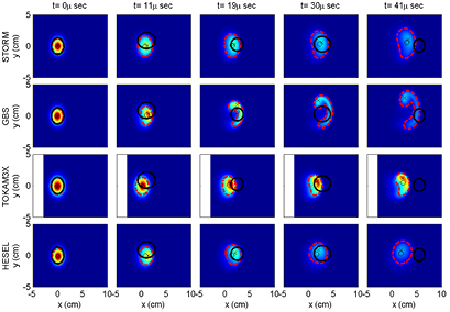
Figure 8. Time evolution of the density in the drift plane located at the midplane for filament 1, case (1). Different rows correspond to different codes, all of which use the cold ion approximation. The thick circles represent the position and size of the measured filament. Note that here the mean plasma rotation is removed from the poloidal velocity of the filament, see section 4.2. The X marks and the small circles show the position of the maximum and of the center of mass respectively. The dashed contour lines correspond to  and delineate the (arbitrary) boundary of the filament.
Download figure:
Standard image High-resolution imageAll codes follow the same trends, as demonstrated in the top and central panel of figure 9 which compare the position of the maximum density and of the center of mass as a function of time for filament 1, case (1). It is interesting to note that, in the initial phase of its evolution, the TOKAM3X filament accelerates less than the STORM and GBS ones but its terminal velocity is consistent with the other two codes. Inspection of the potential field associated with the  motion of the filament shows that the TOKAM3X simulations initially generate a monopole in ϕ that turns into the bipolar structure observed in the other non-isothermal codes only later. This might be due to the absence of the electron inertia in Ohm's law which implies that in TOKAM3X the initial potential immediately tends to adapt to the pressure field, thus affecting the following evolution of the potential dipole. In addition, the decrease of the maximum density at the midplane is very similar in STORM, GBS and HESEL, and significantly faster than in TOKAM3X, see bottom panel of figure 9.

Figure 9. Top panel: position of the maximum of the density at midplane for filament 1, case (1) as a function of time. Central panel: same as top panel but for the center of mass position. The simulated maxima of the density and the position of the center of mass are represented with triangles and circles respectively (the color of the markers is the same between the two panels). Bottom panel: time evolution of the maximum density at midplane for filament 1, case (1).
Download figure:
Standard image High-resolution imageThe simulations discussed in this section display features that are representative of the remaining cases of filament 1 and 2. When an initial temperature perturbation is imposed, filaments appear to be systematically slower in TOKAM3X than in the non-isothermal codes, due to the fact that in the former only the perturbed density contributes to the pressure drive. STORM and GBS appear to be largely in agreement when the radial and bi-normal position of the center of mass of the filament are concerned. The difference in the internal structure of the filaments in the two codes is attributed to the fact that STORM adapts the perpendicular collisional diffusion coefficients to the local values of the density and temperature, while GBS uses a constant value. This hypothesis was tested by performing a simulation with STORM without the local corrections and the result was that the filament was less rounded and developed a curl similar to the one found by GBS.
The HESEL simulations used in the rest of the paper include hot ion dynamics. This is a defining feature of the standard HESEL model, which also employs a reduced slab curvature term,  , and poloidal averages in the vorticity sink term, which becomes
 ![$2/{{c}_{s}}\left[1-\exp \left(\Lambda -{{\langle \phi \rangle}_{y}}/{{\langle {{T}_{e}}\rangle}_{y}}\right)\right]$](https://content.cld.iop.org/journals/0741-3335/58/10/105002/revision1/ppcfaa35c2ieqn107.gif) . The rationale behind the averages was to represent the physics of filaments in the inertial regime while retaining the effect of sheath currents on the mean fields. It is therefore useful to compare the results of a typical simulation done with the model used for the benchmark and one done with the standard HESEL model. Figure 10 shows such a comparison for filament 1, case (1). Here, the top row displays the evolution of the cold ion filament, the middle row the hot ion case with non averaged vorticity closure (like in the cold ion case) and the bottom row the hot ion poloidally averaged vorticity closure (as used in the standard HESEL model).
. The rationale behind the averages was to represent the physics of filaments in the inertial regime while retaining the effect of sheath currents on the mean fields. It is therefore useful to compare the results of a typical simulation done with the model used for the benchmark and one done with the standard HESEL model. Figure 10 shows such a comparison for filament 1, case (1). Here, the top row displays the evolution of the cold ion filament, the middle row the hot ion case with non averaged vorticity closure (like in the cold ion case) and the bottom row the hot ion poloidally averaged vorticity closure (as used in the standard HESEL model).

Figure 10. HESEL simulations with different models. Top row: time evolution of a filament at midplane with cold ions, larger curvature drive and non poloidally averaged vorticity sink. Middle row: same as top row for hot ions and with smaller curvature drive. Bottom row: same as middle row with poloidally averaged vorticity sink.
Download figure:
Standard image High-resolution imageThe hot ion simulations gives a larger radial displacement. This, however, is understood in light of the higher filament pressure. The poloidal averaged closure, however, produces larger radial velocities than the non averaged case. In addition, the shape of the filament becomes more elongated in the bi-normal direction and less up-down symmetric due to the increased vorticity induced by the ion temperature field [49]. The bi-normal motion is quite different among the three cases, both in magnitude and direction. While the cold ion filament drifts in the ion diamagnetic direction, like the 3D codes, the non poloidally averaged closure generates a motion in the electron diamagnetic direction. The averaged closure starts like the cold ion case but ends its evolution drifting in the electron direction, due to the asymmetric structure of the filament.
4.2. Comparison with the experiment
Using the synthetic diagnostic discussed in section 3.3, we calculated the radial and toroidal position of the two simulated filaments for each of the three amplitude combinations consistent with the experimental light emission. Figure 11 compares the simulated radial position of filament 1 (left column) and filament 2 (right column) with the experimental values.

Figure 11. Comparison between the simulated and the experimental radial position of the filament as a function of time. The left column represents filament 1 and the right column filament 2. Case (1) to (3) are given from top to bottom. The solid curve represents the experimental data, the shaded area its uncertainty and the dashed curves the results from the codes.
Download figure:
Standard image High-resolution imageCase (1) and (2) are very similar to each other and both provide a good match with the measurements of filament 1 for most of its life. This suggests that the electron temperature in this filament is not much higher than the background's, see table 1. On the other hand, the codes fail to reproduce the final stage of the evolution of the filament. This, however, might be due to the fact that the experimental data display an internal restructuring of the filament in the last stage of its evolution, which might affect the measurement of its position. While the STORM and GBS simulations lie within the experimental errorbars for  of the total evolution time, the displacement predicted by TOKAM3X remains systematically below. However, this is mostly caused by the slow acceleration in the initial phase described in the previous section, while the final velocity of the filament is similar to those calculated by the other 3D codes. For the slower evolution of filament 2, the predictions of all 3D codes are well within error bars only for case (3), which suggests that the lower radial velocity of this perturbation might be explained by its larger temperature above the background, see table 1.
For both filaments, the HESEL simulations are systematically predicting larger displacements due to the contribution of the ion temperature. However, the fact that no direct measurements of the ion energy are available for the cases treated implies that the numerical results with finite Ti dynamics are implicitly subject to large errorbars. GBS simulations were performed to assess the importance of the hot ion effects in 3D. It was found that the filaments' radial velocity was half the one calculated by HESEL with the poloidally averaged closure, but it was almost identical to the HESEL simulations with non-averaged closure. The GBS hot ion results predicted perturbations moving radially around 60–70 faster than the cold ion case for filament 1 and around 100
 faster for filament 2. This implies that even assuming
  , both filament 1 and filament 2 would be pretty close to the experimental measurements and very close to the upper level of the error bars. This suggests that the ion temperature might be less high than our rough estimate or that our codes require additional physics that might slow down the filaments. On the other hand, our results also indicate that cold ion simulations are reliable in calculating the radial velocity within a factor less than 2.
The comparison with the toroidal velocity is more complicated and less direct since the rotation of the background plasma is unknown. Assuming that it does not change significantly in the ∼0.5 m s between filament 1 and 2, we compare the experimental and numerical evolution of the difference in the toroidal position (with respect to the initial value) of the two filaments. This procedure removes the mean rotation, which is identical for both filaments and captures only the intrinsic motion in the toroidal direction. An underlying assumption in this procedure is that the mean flow is not significantly sheared in the ∼5 cm gap between the separatrix and the wall shadow. While no direct measurements are available for the discharge examined, recent probe measurements of the upstream profile of the electrostatic potential in MAST [50] suggest that the  flow has only weak variations in the region of interest, thus confirming our assumption. In particular, we start tracking and simulating filament 1 and 2 when their centers of mass are 1.5 cm and 1 cm outside the separatrix (compare with figure 4) and figure 10 in [50] suggests that beyond 0.5–1 cm the poloidal and toroidal plasma velocity is roughly constant.
For convenience, we introduce the notation  for the difference in toroidal angle between case (m) of filament 1 and case (n) of filament 2. Figure 12 shows a comparison between the experimental and the numerical
  for all the nine possible combinations (two filaments with three cases each). According to STORM and GBS, filament (1), case (2) and filament (2), case (3), represent the best fits for the toroidal motion as the numerical predictions are within the errorbars of the experimental data and capture the right trends. Importantly, if different combinations of cases are used, the agreement with the observations worsens significantly, thus reinforcing the idea that filament (1) is better described by case (2) and filament (2) by case (3). Using these results, we can evaluate the intrinsic toroidal rotation of the filament (from the simulations), which is 0.2–1 km s−1, and the mean SOL plasma rotation, which is around 3 km s−1 (from the measurements minus the filament rotation). These values are in agreement with previous observations in MAST [35]. The TOKAM3X simulations always predict a similar toroidal rotation for the two filaments, which is not surprising since this quantity is regulated by the temperature dynamics, missing from the version of the code used for this work. The HESEL simulations predict an opposite trend with respect to the other codes. This is due to the fact that rotation is intrinsically linked to 3D effects, which play a dominant role in setting the bi-normal velocity [51].

Figure 12. Difference in toroidal angle between filament 1 and filament 2 for all possible combination of cases. The subplots show the time evolution of  with m increasing from left to right and n increasing from top to bottom. The solid line is the experimental measurement, the dashed lines represent the output of the four codes, with the same conventions of figure 11. The errors on the experimental measurements are taken as half the bi-normal size of the filaments (averaged). Note that the legend is omitted as it is the same as that of figure 11.
Download figure:
Standard image High-resolution imageFinally, we note that most of the internal structures of the filaments are lost in the process of generating the synthetic signals. This is due to line integration effects and the spatial resolution of the camera, which remove many fine scale details. A consequence of this is that it is sometimes difficult to discriminate between, for example, STORM and GBS simulations, which generate filaments with different shapes, but moving with similar velocities. Symmetrically, these results highlight the limitations of the experimental technique, which cannot resolve small scale details in the filament.
4.3. Sensitivity studies
To determine the robustness of our numerical results, we performed several sensitivity studies. Their aim was to provide a general quantification of the effect of the measurement uncertainties on the conclusions of the previous section.
As mentioned in section 2.2, the relative error on the filament perpendicular size is around  . One simulation with
  and
and  1.5 times larger and one 1.5 times smaller with respect to the nominal value for filament 1, case (2) were carried out with STORM. We found that the radial velocity increases with perpendicular size, suggesting that the filament is in (or close to) the inertial regime. This is confirmed by the fact that the critical perpendicular filament size separating inertial and sheath regimes (see e.g. [17, 41]) is for the case treated
  , i.e. larger than the filaments we investigated. The peak velocity of the center of mass is 1.5 times smaller for the small filament, while it is 1.15 times larger for the large filament, which implies that the velocity scales less than linearly with the perpendicular width, as expected in the inertial regime. The discrepancy from a square root dependence suggests that viscous effects might play a role in determining the dominant balance in the vorticity equation [44].
An element of uncertainty in the initialisation of the simulations is the parallel size of the filament, which cannot be measured directly with the technique we employed. It is reasonable that the density associated with a filament emerging from the core in the proximity of the separatrix cannot have a parallel length scale much longer than the upper X-point to lower X-point distance along the flux tube. However, particularly ballooned perturbations might constrain the filament on a ∼60° arc around the midplane [22, 42]. To investigate the effect of different parallel extensions of the filament, we performed STORM simulations with  and
and  . The result was that a parallel front closer to the target leads to higher radial velocities, in particular, Vr was 1.3 times the reference velocity when
  and 0.75 times when
  , yielding an almost linear scaling.
Another assumption of this work is the choice of neoclassical perpendicular diffusion coefficients, but rigorous theory of collisional transport in the open field line region of a toroidal configuration is not yet available. To study this issue, STORM, GBS and TOKAM3X have performed simulations of filaments 1 and 2 with perpendicular diffusion coefficients orders of magnitude different (∼10−1 m for STORM, ∼10−3 m
 for GBS and ∼10−2 m
 for TOKAM3X). An interesting result was that the radial and toroidal velocities of the center of mass of the perturbation did not change much within this large range of dissipation parameters, in agreement with what was found in the TORPEX validation work [13]. On the other hand, the internal structure of the filament was completely different, with smaller scale structures forming and fragmenting in low dissipation cases (see also [52]). Interestingly, GBS showed an increase of the maximum density value in the filament at midplane as a function of time. This was due to the compression of the plasma in the perpendicular front of the filament, which become much thinner and elongated. This effect was completely removed by the smearing of the internal structures of the filament caused by MAST relevant diffusion.
4.4. Additional physics insight
The investigation of different combinations of initial density and temperature amplitudes in the filament generated a number of interesting observations. For the parameters investigated, the parallel dynamics of the different fields evolved on quite disparate time scales. The discussion below relies mostly on STORM simulations, which include in all the equations the fast time scales associated with the electron response.
On fast time scales of less than a μs, the parallel pressure gradients strongly drive the light electrons towards the target, starting from the front region where the X-point would be. We can estimate that the normalised acceleration scales like  . The parallel advection of the velocity tends to increase V along z, while maintaining the condition V = 0 at the symmetry plane. This has the consequence of driving an intense monopolar current, that induces perpendicular polarisation currents through the vorticity equation to preserve quasi-neutrality, even in the region between the end of the filament and the target. These currents are carried almost exclusively by the electrons, with the heavy ions remaining a passive substrate for most of the simulation and starting to move only towards the end in the parallel pressure gradient region. After the formation of this monopole in ϕ, the drive of the diamagnetic currents induced by the pressure gradients in the perpendicular plane induces an electric field polarised in the bi-normal direction, providing the
  velocities that propel the filament in the radial direction. In around
  s the dipolar structure propagates through the background all the way to the target.
Associated with the polarisation current is the creation and propagation of the electrostatic potential, which is therefore induced in the target region after only a few μs. As the simulations are electrostatic, the propagation of the electrostatic potential is not mediated by Alfven waves. It is instead due to the parallel propagation of the electrons, which can only be observed when their inertia is retained in Ohm's law.
On a slightly longer time scale, the excess temperature in the filament flows towards the target through the efficient parallel electron heat transport, see figure 13. In the simulations the electron temperature perturbation reaches the target in ∼2.5 μs, compatible with the estimate  μs. Note that the former time was estimated by checking when the maximum value of the temperature perturbation at the target was equal to the maximum value of the temperature at the midplane. The evolution of Te produces a transient heating of the target, which, before returning to the background level, can be hotter than the filament at the midplane.

Figure 13. Top row: time evolution of the normalised density perturbation,  , in 3D for filament 1, case (2) as calculated by STORM. The contours are calculated between 0.1 and 1 in steps of 0.1. Negative values of
  can be seen close to the target. The negative contours are calculated between −0.1 and −0.025 in steps of 0.025 (note the different scale). Bottom row: same as top row for the normalised temperature perturbation,
  . Temperatures below the background can be seen in the target region (but not at the midplane, where they are below −0.025). All lengths are in cm and the frames are
  s apart (the first frame is the initial condition).
  and
and  are the maxima in the whole domain and over all the time history.
Download figure:
Standard image High-resolution image
Another interesting observation is related to the perpendicular structure of the temperature perturbation. For case (2), which has a moderate initial Te amplitude, the filament generates temperatures slightly below the background value both at the midplane and at the target, see figure 13. This is not due to parallel adiabatic expansion, as the generation of the negative temperature fluctuation occurs on faster time scales than those characterising ion dynamics. Note that the temperature reduction at the target is of the order of 2.5% of the background, while upstream is even smaller, which suggests that this effect might be difficult to measure. If the initial temperature perturbation is sufficiently large, such as in case (3), the density profile becomes hollow as the faster sound speed in the center of the filament leads to a faster exhaust of the particles towards the divertor. This effect is observed in STORM but not on GBS, probably due to the fact that GBS' parallel heat conduction term does not depend on the local temperature. In addition, Boltzmann spinning [51, 53] induces a rotation of the filament on its axis, creating an annular density structure. A more theoretical analysis of the temperature effects can be found in [39].
Only on longer time scales, of the order of the simulation time (∼50 s), the parallel motion of the density perturbation, related to the ions, becomes evident, see figure 13. The ions remain stationary for a large part of the simulation and they start accelerating due to the parallel electric field induced in the front of the filament. By the end of the simulations, the parallel front of the density never reaches the target, which is consistent with the fact that the parallel transit time is of the order of
  μs. On the other hand, a small density finger can slightly protrude ahead of the front due to the transient associated with the initial acceleration of the electrons. Despite the fact that the upstream density is exhausted slowly, the target density is affected by the presence of the filament on the electron time scales. Indeed, as the target region heats up rapidly, also the local sound speed increases and induces a more efficient draining towards the sheath. This, in turn, efficiently removes the density, so that a region of low density (lower than the background) appears in front of the target, as shown in figure 13.
While some of the dynamics described above is due to the initial imbalance caused by the lack of potential and velocity perturbations at the beginning of the simulations, the time scales discussed are representative of transient phenomena that could occur in SOL turbulence. In particular, we expect the density and temperature evolution to be representative of ballooned filaments that separate from the core at the X-points or above, so that the fields have to propagate at least along the divertor leg. Similarly, also the parallel velocity perturbations and relative currents should develop in a similar way as described here. However, the behaviour of the electrostatic field might be significantly more complicated as we expect the filament to separate with an already formed electric field associated with it. On the other hand, our discussion clarify some of the mechanisms for the potential propagation from filamentary structures in the electrostatic approximation.
5. Summary and conclusions
We presented a comprehensive experimental and numerical study of the physics of SOL filaments in MAST. Through new techniques based on the analysis of the visual light emitted by the plasma edge, we measured several properties of two filaments, among which their perpendicular size, their radial and toroidal displacement and the relation between density and temperature perturbations. A numerical campaign was carried out with four numerical codes to simulate these filaments. Our approach was to seed the filaments in the simulations in order to investigate the dynamics of isolated structures. The purpose of the simulations was twofold: to validate the codes against experimental data in tokamak conditions (previous work of similar nature [13] was performed in a simple magnetised torus configuration) and to gain insight into the physics of the filaments that could not be directly measured.
We found that, for equal conditions, the codes were in acceptable agreement as far as the radial motion of the filament is concerned. In particular, in the isothermal case, the final velocities from the four codes were close to each other. On the other hand, the exhaust of the particles occurred at different rates in TOKAM3X, while HESEL, STORM and GBS obtained similar trends.
The comparison with the experimental data showed agreement in the radial position within the error bars for both filaments considered. The difference in the intrinsic rotation of the two filaments was captured by GBS and STORM and was shown to rely on temperature effects (which were missing in the version of TOKAM3X used for the comparison). In addition, the analysis allowed interpreting the experimental data, suggesting that filament 2 was generated with a larger temperature perturbation than filament 1, which affected its cross field dynamics and explained why the perturbation had a much slower radial motion despite the similarity in the amplitude and perpendicular size. Also, we were able to estimate the SOL toroidal rotation, ∼3 km by removing the intrinsic motion of the filaments from the total experimental measurement.
Sensitivity studies were carried out to understand how robust the numerical results were and to estimate the uncertainties on the simulations' outputs. The parallel and perpendicular size of the filaments affect their evolution, but not dramatically, so that the assessed uncertainties in the initialisation of the codes do not affect the conclusions of this work. Similarly, the collisional diffusion changes the internal structure of the blob, but it has a weak effect on its radial displacement.
As an additional benefit, the simulations helped to shed some light on the 3D dynamics of the filaments, especially clarifying the way the temperature and potential fields propagate towards the target. Interesting effects associated with the electron response were identified, and allowed interpreting some of the discrepancies between the codes, for example the slow initial acceleration of TOKAM3X.
The biggest element of uncertainty in our work is the role of the ion temperature, which is not directly measured. Under the assumption that it is twice as large as the electron temperature, the motion of the HESEL hot ion filaments with poloidally averaged closure is significantly larger (a factor (3) than the cold ion predictions and cannot explain the difference in the toroidal rotation. However, 2D simulations performed with HESEL with non-averaged closure and 3D simulations carried out with GBS showed good agreement with each other and a much smaller discrepancy between the cold and hot ion models, the latter displaying filaments roughly 60–100 faster in their radial motion, which is only slightly above the experimental error bars.
The precision of the validation performed in our work could certainly be increased by obtaining more precise estimates for the amplitude of the filament. In this respect, coupling the visual camera images with reciprocating probe data from the same filament would generate two signals produced by different combinations of density and electron temperature, which could therefore be calculated independently. Similarly, the use of mirror, triple, ball pen, emissive or retarded field energy analyser probes could provide a measurement of the temperature of the electrons and, for the latter, also of the ions. The uncertainty on the ion temperature is an important limitation of our work, as it affects the pressure drive of the filament.
In general, filaments in the SOL have a rather broad statistical distribution of sizes, amplitudes and velocities [10, 11, 35]. The filaments we selected are probably representative of the high amplitude, large size part of the population, as these features produce signals that are easier to detect in the camera images. Also, we chose blobs that were sufficiently isolated to ensure that the seeded simulations were representative. In general, it would be interesting to assess the importance of the interaction between filaments, which might occur through the electrostatic fields they generate, although this goes beyond the scope of the present work.
Finally, another limitation of the work is the absence in the simulations of magnetic [54] or velocity shear effects, which could affect both the internal stability of the filament and their motion. While indirect experimental estimates of the magnetic shear are available through magnetic reconstruction, the velocity profile in the SOL is considerably more difficult to quantify. However, previous measurements [50] suggest that the velocity shear might be significant in the proximity of the separatrix but it quickly decays further out, where our filaments were tracked and simulated. The study of these effects is therefore left for future studies.
Acknowledgments
FM acknowledges useful discussions with Dr A Kirk and thanks Dr J Harrison for carefully reading the manuscript. Camera calibrations were performed with the CALCAM code, developed by Dr S Silburn and Dr J Harrison, whom we gratefully acknowledge. This work has been carried out within the framework of the EUROfusion Consortium and has received funding from the Euratom research and training programme 2014–2018 under grant agreement No 633053, from the RCUK Energy Programme (grant number EP/I501045) and from the Swiss National Science Foundation. Part of the simulations presented herein were carried out using the HELIOS supercomputer system at Computational Simulation Centre of International Fusion Energy Research Centre (IFERC-CSC), Aomori, Japan, under the Broader Approach collaboration between Euratom and Japan, implemented by Fusion for Energy and JAEA, and part were carried out at the Swiss National Supercomputing Centre (CSCS) under Project ID s549. This work was granted access to the HPC resources of Aix-Marseille Université financed by the project Equip@Meso (ANR-10-EQPX-29-01) of the program 'Investissements d'Avenir' supervised by the Agence Nationale de la Recherche. To obtain further information on the data and models underlying this paper please contact PublicationsManager@ccfe.ac.uk. The views and opinions expressed herein do not necessarily reflect those of the European Commission.