
Abstract
The Gravity Probe B mission provided two new quantitative tests of Einstein's theory of gravity, general relativity (GR), by cryogenic gyroscopes in Earth's orbit. Data from four gyroscopes gave a geodetic drift-rate of −6601.8 ± 18.3 marc-s yr−1 and a frame-dragging of −37.2 ± 7.2 marc-s yr−1, to be compared with GR predictions of −6606.1 and −39.2 marc-s yr−1 (1 marc-s = 4.848 × 10⁻⁹ radians). The present paper introduces the science, engineering, data analysis, and heritage of Gravity Probe B, detailed in the accompanying 20 CQG papers.
Export citation and abstract BibTeX RIS

Content from this work may be used under the terms of the Creative Commons Attribution 3.0 licence. Any further distribution of this work must maintain attribution to the author(s) and the title of the work, journal citation and DOI.
1. Overview: space, relativity, and cryogenics
This and the following 20 papers describe the NASA Gravity Probe B Mission launched 20 April 2004, which yielded two entirely new tests of Einstein's theory of gravity, general relativity (GR), from the frame-dragging and geodetic precessions of gyroscopes in Earth's orbit.
In GR rotating matter drags the framework of spacetime around with it. Frame-dragging was first studied in 1918 by Lense and Thirring [1] who looked for, but could not detect, a dragging of the Moons of Jupiter. In 1959, two years after the launch of the world's first artificial satellite, the Russian Sputnik, Schiff [2] and Pugh [3] independently proposed searching for a related effect Ωfd on gyroscopes in Earth orbit, with an accompanying geodetic term Ωg, ∼168×larger, from spacetime curvature (the circumference of a circle around a gravitating body being <2πr). In the polar orbit of figure 1 the two effects are at right angles; taking  as the gyro spin vector, Schiff found a drift rate
  where
where

Figure 1. The two Schiff effects. North–South, East–West relativistic precessions with respect to the guide star IM Pegasi for an ideal gyroscope in polar orbit around the Earth. Download figure: the Earth's mass, moment of inertia and angular velocity, r and v the radius and velocity in the orbit. Other theories, notably the once-popular Brans–Dicke scalar–tensor theory, gave different results. Frame-dragging may be viewed as a 'gravitomagnetic' effect analogous to the magnetic field generated by a rotating electrified body. Paper 2 in this issue [19] has more on the significance of the two terms; paper 3 [20] details constraints on one class of alternative theories.
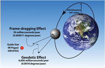
The Schiff frame-dragging in figure 1 is 39 marc-s yr−1, a factor of four below the 156 marc-s yr−1 Lense–Thirring effect, since the gyroscope drag reverses over the equator. In 1975 van Patten and Everitt [4] showed that while results from a single satellite measurement are limited by the much larger Newtonian effect from the Earth's oblateness, cross-ranged data from two counter-orbiting satellites in polar paths around the Earth could give the Lense–Thirring ΩLT to 1%. A reported result from Ciufolini and Pavlis [5] (2009) for the 19° co-inclination LAGEOS satellite depended on computing out the oblateness term to better than a part in 107, as also in 2009 for data from the GRACE satellite [6]. A review by Iorio 'an assessment of the systematic uncertainty in present and future tests of the Lense–Thirring effect with Satellite Laser Ranging' [7] may be consulted. For frame-dragging in astrophysics see Thorne Gravitomagnetism, Jets in Quasars, and the Stanford Gyroscope Experiment [8], and two recent papers by Reynolds [9].
In computing the predicted Ωfd, Ωg each quantity in equation (1) was known: the instantaneous orbit velocity and radius from GP-B's on-board GPS detector; the mass, moment of inertia, and angular velocity of the Earth from geophysical and astrophysical data. There were five relevant terms to consider: (1) the Ωfd frame-dragging; (2) the Ωg geodetic effect; (3) the 19 marc-s yr−1 de Sitter [10] effect, also geodetic, from motion around the Sun; (4) a 7 marc-s yr−1 correction to Ωg from the oblateness of GP-B's orbit around the Earth; (5) the gravitational deflection of IM Pegasi's light by the Sun, reaching 14.4 marc-s on 11 March. The Ωfd just quoted incorporates the de Sitter effect; the Ωg includes the correction for orbit-oblateness.
The GP-B Spacecraft was a major axis spinner rolling with 77.5 s period about the line to IM Pegasi. Its main structural element was a 2441  superfluid helium Dewar, designed for 16 month on-orbit hold-time at 1.8 K, with a removable ultra-high-vacuum inner Probe holding the Science Instrument Assembly (SIA). Communication to the ground took two forms: Spacecraft operations by the NASA Tracking and Data Relay Service Satellite; high speed science data transmitted 3 to 4 times a day to stations at Svarlbad, Norway, Wallops Island, Virginia, Poker Flats, Alaska, and McMurdo Sound, Antarctica; and thence via NASA Goddard Center to the Stanford Mission Operations Center (MOC) described below in section 3.3.
GP-B hinged on nine essentials (section 1.2): three cryogenic, three met by the low-g of space, and three by spacecraft roll. These led to 12 fundamental requirements defining management and instrument layout. Consider GP-B's uniquely exact Attitude/Translational Control system. At 642 km altitude, air drag and solar radiation pressure made a ∼10−8 g acceleration on the Spacecraft. The Dewar's boiloff gas vented through 'proportional thrusters', referred to one of GP-B's four gyroscopes as a proof mass to measure the acceleration, reduced this to a mean value well below 10−10 g, making the satellite effectively drag free. Central to the gyroscope design were first low-g suspension, second an angular readout capable of resolving a 1 marc-s change in spin direction in 10 h, and third the ability to apply a spin-up torque and then switch it off by 15 orders of magnitude. Confidence was strengthened by the use of two distinct data analysis methods, referred to as Algebraic and Geometric, explained in section 4.
1.1. Cryogenics and the SIA
Figure 2 is the SIA, a 0.62 m long quartz block structure containing four gyroscopes two spinning clockwise and two counterclockwise, attached to GP-B's 0.14 m aperture, 3.94 m focal length reference telescope, all subject to severe constraints on pressure, cleanliness, stability, and magnetic shielding. The total SIA length was 1.04 m. The goal was a net gyro drift-rate ∼10−11 deg h−1 for a fourfold test of Ωfd, Ωg: 109 times beyond absolute rates and 106 beyond 'modeled' rates of 1964 navigation gyroscopes. The gyroscope was a 38 mm diameter electrically suspended sphere coated with superconductor, spinning typically at 80 Hz. On Earth the voltage over the 30 μm electrode-rotor gap was 700 V; on orbit it was 0.2 V. With torque from residual out-of-roundness of the rotor scaling as V2, gyro drift from this cause was lowered on orbit by ∼107, with further reduction from Spacecraft roll. Central to the design of the experiment was a new form of gyroscope readout based on the London magnetic moment in the spinning superconductor.
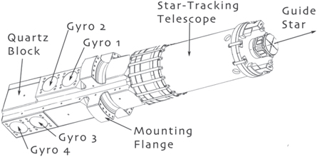
Figure 2. Science Instrument Assembly: four gyroscopes, mounted in line within 25 μm of the telescope boresight, yielded four independent measurements of the two relativity terms Ωg, Ωfd.
Download figure:
Standard image High-resolution image1.2. Nine essentials for mission success
Nine essentials drove GP-B's technologies: A. Space: (1) greatly reduced gyro drift through not having to suspend the rotors against gravity, (2) separated Ωfd and Ωg in polar orbit, increasing Ωg by 12.4 over a ground-based test, and (3) eliminated 'seeing' in the guide star measurement. B. Cryogenics: (4) allowed the use of superconductivity for gyro readout and shielding, (5) greatly aided ultra-high vacuum operation, and (6) improved the SIA's thermal stability. C. Roll: (7) minimized 1/ƒ noise in the gyro readout, (8) symmetrized the telescope output, and (9) provided additional averaging of certain gyro torques. The 12 fundamental design requirements that followed are listed in section 2.4.
1.3. Ground-based versus on-orbit testing
The SIA and gyroscopes underwent 150 000 h of ground-based testing, some cryogenic, some at room temperature, linked to a succession of on-orbit operations and tests with the flight partitioned into three phases: set-up, science, and post-science calibration.
Set-up, detailed in section 3.2, was a comprehensive 129 day learning process beginning with alignment of the rolling Spacecraft on the guidestar IM Pegasi. Science (352 days) and post science calibration (43 days) revealed, in addition to GR data, three surprises:
- (1)rapid damping of rotor polhode motions (∼100 days versus the expected >103 yr);
- (2)a ∼103 higher than expected misalignment torque;
- (3)a roll-polhode resonance torque when the gyroscopes' changing polhode rates came into resonance with the satellite roll.
On-orbit and ground-based tests traced all three to coupling between patch charges on the rotors and housings. Spherical as they were mechanically, the rotors and housings had irregular electrical surfaces.
Post-science calibration had two aspects, enhancement and modeling. Take surprise 2, the higher than expected misalignment torque, calibrated post science by pointing the Spacecraft to stars 0.4°–7° away from IM Pegasi. Drift rates increased in known ratios; modeling became possible, with a cross check from the ±20.496 arc-s annual aberration in the apparent position of IM Pegasi from the Earth's motion around the Sun. Other potential disturbing effects were checked post science by linearly increasing the offsets causing them, thereby either showing them to be negligible or providing on-orbit scaling. Take gyro readout. Required is an angle; the measurement was a voltage. How accurate in marc-s V−1 was the scale factor? Ground-based calibration was not easy, nor was it clear that it would survive launch. Again aberration, this time the 5.1856 arc-s orbital term from GP-B's motion around the Earth, allowed an on orbit calibration good to 1 part in 105.
Most requirements came in pairs. Take, for example, the 'mass unbalance' torque fδr on a not quite homogeneous rotor, f being acceleration and δr the distance between the rotor's centers of mass and geometry. The mean transverse on-orbit f turned out to be ∼4 × 10⁻¹² g, the homogeneity needed was δr/r <10−5; f was checked on orbit, δr by applying the classic Lorenz–Lorentz density/refractive index formula to ground-based measurements in a matching index refractometer developed for GP-B at the University of Aberdeen, Scotland [11].
1.4. Quick view of science results
Table 1 gives the result for each gyroscope in marc-s yr−1. Within the one-sigma limit they agree and confirm the Schiff geodetic and frame-dragging predictions to 0.3% and 18%. A truth model by Turneaure [12] gives prospects of further improvement.
Table 1. Results.
| Source | RNS (marc-s yr−1) | RWE (marc-s yr−1) |
|---|---|---|
| Gyroscope 1 | −6588.6 ± 31.7 | −41.3 ± 24.6 |
| Gyroscope 2 | −6707.0 ± 64.1 | −16.1 ± 29.7 |
| Gyroscope 3 | −6610.5 ± 43.2 | −25.0 ± 12.1 |
| Gyroscope 4 | −6588.7 ± 33.2 | −49.3 ± 11.4 |
| Joint | −6601.8 ± 18.3 | −37.2 ± 7.2 |
| GR prediction | −6606.1 | −39.2 |
In what follows: section 2 covers the experiment's overall design; section 3 the Spacecraft and mission operations; section 4 the science data, analysis models, and results.
2. Space, cryogenics, and the 12 fundamental requirements
We cover here gyroscope design, telescope/SIA layout, cryogenic payload layout, and the 12 requirements which brought rigor to the design and clarified working relations between the three cognizant organizations: NASA, Stanford University, and Lockheed Martin.
2.1. The gyroscope
Our first NASA-funded task in 1964 was to evaluate known gyroscope concepts: ring-laser, He3 nuclear, 'dry tuned' gyros with spring-mounted spindles, and nearest by far to GP-B's need, the electrically suspended gyroscope (ESG) invented by Nordsieck in 1953 [13]. By the V2 argument of section 1.1, ESG performance should improve on orbit, but how much? The most advanced ESG, manufactured by Honeywell, with hollow beryllium rotor, eddy current spin-up, and optical readout of the spin direction was two orders away from measuring even Ωg. For GP-B, Ωg was visible in the raw data from each of the four gyroscopes, as seen in figure 15 below. Figure 3 is the GP-B gyroscope, also an ESG but cryogenic, spun up by helium gas, and with the London moment readout mentioned earlier. We start with the rotor.
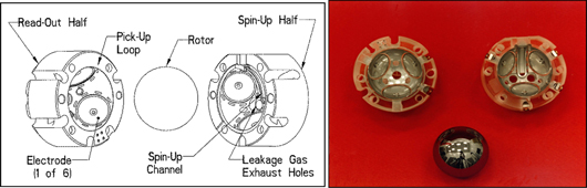
Figure 3. Exploded view of GP-B gyroscope. The rotor and two halves of the housing showing support electrodes, spin-up channel, and the pick-up loop for the London moment readout.
Download figure:
Standard image High-resolution image2.1.1. The rotor
Rotor development faced three issues: homogeneity, sphericity and size (paper 4, [21]). Nordsieck's gyroscope had a 76 mm rotor; the Minneapolis Honeywell one was 38 mm; Pugh's proposed relativity gyroscope had 1 m diameter. A paper from 1890 by Boys [14] on scaling laws for the Cavendish experiment is relevant. From dimensional arguments Boys established that the accuracy of that experiment would gain by making the apparatus smaller. For GP-B it was otherwise. Torques on rotors fall into two categories: those related to surface area and those related to volume. Over a fair range of radii, drift rates for surface-dependent and volume-dependent torques scale as r(s−1) and rv, where s and v lie between 0 and 1. The choice of a 38 mm rotor hinged not on torques but laboratory testing and SIA layout.
Early studies called for a rotor round to 0.4 μin (10 nm)—rounder by a factor of 5 than the best industrial spheres. Figure 4(a) is the advanced lapping machine developed at NASA Marshall Center. Figure 4(b) is a contour map of one rotor, with peak-to-valley variations of 0.74 μin (18 nm) from 17 great circle measurements with a Talyrond roundness measuring instrument, using a reversal technique due to Southwood7 to remove errors from out-of-roundness of the Talyrond spindle. Expanded to the size of the Earth the rotor's highest mountain to deepest valley would be 3 m. To generate the London moment without unbalancing the rotor, it was coated with a 1.25 μm layer of niobium, uniform to 2%.
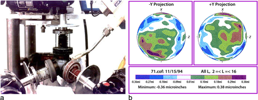
Figure 4. Lapping and measurement of a GP-B gyroscope rotor. (a) Is the NASA MSFC lapping machine with the sum of the four lap-spin vectors held always to 0 with cyclic reversal every 12 s; (b) is a map of rotor shape based on 17 Talyrond great circle measurements.
Download figure:
Standard image High-resolution image2.1.2. Suspension
Six needs defined the suspension system: (1) eight orders of magnitude working range to support rotors on Earth and in orbit (2) rapid level switching during emergencies, (3) holding center with minimal control to keep support-torque drifts two orders below Ωfd, (4) ability to apply directed torques after spin-up to align the rotor within 10 arc-s of the spacecraft roll axis, (5) no interference with the London moment readout, (6) provision of the on-orbit acceleration signal to make the satellite drag-free. Paper 5 [22] details the design; an alternative briefly considered was superconducting magnetic suspension then under development at two institutions, JPL and GE Schenectady. Here, a point of principle deserves remark. Suspending a sphere means applying uneven pressure over its surface; such pressure on an out-of-round sphere causes a torque. Only for some quite special reason might one support mode yield lower torques than another. With electrical suspension, it is that the sum of the six energies under the support electrodes be independent of rotor orientation, a condition Honeywell had approximated in two control modes, 'sum-of-the-energies' and 'sum-of-the-squares', relevant for navigation gyroscopes but not for GP-B. For us, electrical suspension had two great merits: quick adjustment in operating level, and controlled adjustment of centering.
2.1.3. Readout
Performing the mission required a gyro readout capable of resolving 1 marc-s change in spin direction in 10 h (paper 6, [23]). At 80 Hz, a spinning superconducting sphere develops a uniform 6 × 10⁻⁵ gauss 'London field' through its volume. Linked by a four-turn pick-up loop (figure 3) to a Superconducting QUantum Interference Device (SQUID) magnetometer, this provided the readout. Figure 5(a) is a niobium box containing the SQUID with electronics, ready for mounting in the Probe. Figure 5(b) gives power spectral densities from ground-based tests, along with the 1 marc-s in 10 h requirement. At 77.5 s roll period all four readouts eat the requirement.
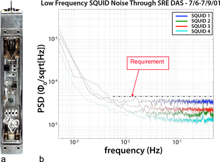
Figure 5. SQUID and support electronics. (a) Enclosed in a niobium box; output signal (b) a 1 marc-s change in spin direction was resolved with the known SQUID 1/f noise in 10 h.
Download figure:
Standard image High-resolution imageTwo essentials were 234 dB attenuation of the twice-orbital variation of the Earth's magnetic field and low trapped flux in the rotors. Our initial aim was zero trapped flux, but even with the most controlled cooling some flux remained and this, far from being a setback, was a gain. Locked to the rotor body, the trapped flux met surprise 1 (polhode damping) by providing a continuous record of the evolving polhode motion and surprise 3 (roll-polhode resonance) by tracking the torques. Transverse superconducting cylinders around each gyroscope, described below under 'overall geometry and shielding' were essential to the 234 dB attenuation.
Unlike the Honeywell optical readout, based on light reflected from a D-shaped pattern at one pole of the rotor [15], GP-B's SQUID readout was sensitive only to second order in rotor centering. More exactly, if x, y, z are the pick-up loop's centering offset from manufacturing errors (10 μm), and δx, δy, δz the shifts in rotor position due to suspension drifts, then with r as the radius of the sphere, the readout shift is  [(2x + y) δz + z (2δx + δy)]. Where an optical readout would have required <8 nm centering stability, GP-B's requirement was 8 μm.
2.1.4. Spin up
Spin up imposed two constraints: (1) the torque had to be applied at a temperature below ∼8 K; (2) it had to be switched off after spin by 15 orders of magnitude. GP-B met both by two special principles, differential pumping and low temperature bakeout.
2.1.4.1. Differential pumping
During spin-up, gas at ∼3 Torr ran at near-sonic velocity through a 5 mm wide spin channel (figure 3) with pressure elsewhere in the housing held to ∼3 × 10⁻⁴ Torr. In final operation the rotors were centered with ∼30 μm spacing; for spin-up each was moved to within ∼10 μm of its channel wall, reducing leakage into the electrode area. The mass flow for each was ∼70 gm, roughly equal to the mass of the rotor; the spin-up time was ∼1 h. Gas from the main channel exited through 25 mm pumping lines in the Probe neck; the remaining 5% being exhausted through the necktube. Critical was the layout of exit valves. One recalls a remark from the great locomotive engineer Churchward, that it is easy to get steam into a cylinder but much harder to get it out again afterwards.
2.1.4.2. Low temperature bakeout
The helium pressure immediately after spin-up was 10−6 Torr, all other gases being frozen out. 'Bakeout' raised the SIA temperature from 2 to 6 K, driving off adsorbed helium in a manner parallel to the 130 °C bakeout procedures in normal ultra-high vacuum systems. The cryogenic region of the Probe was then allowed to cool to 2 K, reaching a final on-orbit operating pressure of <10−14 Torr. A 250 m2 surface area cryopump (figure 9) separately baked out at 10 K, absorbed any gas not exhausted to space. Figure 6 compares ground-based measurements with and without the cryopump.

Figure 6. Low temperature bakeout of gyroscope after spin-up. The data with and without a cryopump was obtained in prior ground-based tests.
Download figure:
Standard image High-resolution imageGas from a pressurized Gas Management Assembly (GMA) bolted to the outer surface of the Dewar entered the Probe by 10 mm spin-up lines linked to the four necktube heat exchangers. Cooled to 6.5 K and rigorously filtered, it was transmitted to each gyroscope in turn, and then vented to space. A contrast with earlier eddy current spin systems is useful. With them, the torque-switching ratio before and after spin-up was 10−9; for GP-B it was 10−15.
2.1.5. Overall geometry and shielding
Centered to within 25 μm on the telescope boresight, each gyroscope was set within a transverse 0.05 m diameter, 0.2 m long superconducting shield, with the shields and readouts referred in pairs to the two telescope axes, the planes for Gyros 3 and 4 being at right angles to those for Gyros 1 and 2. As the Spacecraft rolled around the line to IM Pegasi the amplitude and phase of each SQUID signal provided determinations of Ωg and Ωfd, roll phase being known from the Attitude Reference Platform described in paper 15 [29]. To ensure stability, we developed a unique silicate bonding technique (since widely adopted in the optics industry) based on hydroxide catalysis. 2 K operation in 0 g held thermal/mechanical distortion to the μarc-s level. Numbers are instructive. In 1 g the SIA cantilevered horizontally from its support would have sagged ∼1 arc-s. Similarly, at ambient temperature, either on Earth or on orbit, it would have required ∼105 attenuation of the heat load from the Sun.
2.2. The telescope and SIA
The telescope (paper 8, [24]) was a folded Schmidt–Cassegrain fabricated from fused quartz, with a convex tertiary mirror centered in the primary, and a sophisticated beam splitter assembly on its front end corrector plate, seen in figure 7. The folded design eased the image divider layout and simplified the quartz block interface. Readout was by Si photodiodes set in minute 'inside-out Dewars' self-heated to 72 K. Figure 7(b) is the image divider. Incoming light passed through a beam splitter to form two images coming to separate focus on two roof prisms, with no chips on their dividing edges greater than 25 nm, fabricated by first lapping the future prism flat on one face, then mounting it in weak optical contact with a flat template, taking a second cut at right angles, lapping the joint face, and cleaving the contact, each edge protecting the other. The prisms, like much else in GP-B, originated with the late Davidson.

Figure 7. GP-B telescope. The folded structure (a) with photodiode readout modules at 72 K simplified layout and attachment to the quartz block. The beam splitter (b) allowed separate highly linear X-axis and Y-axis readouts.
Download figure:
Standard image High-resolution imageOur initial SIA design was a four-square array with the gyroscopes crosswise, two to measure Ωg and two to measure Ωfd. The final in-line layout allowed faster roll, reducing 1/f noise in the SQUID readouts as seen in figure 5. Drag-free operation held the mean cross track acceleration to 4 × 10⁻¹² g. Note the expression mean acceleration. With Gyro 1 as proof mass, the Earth's field gradient produced in Gyros 2, 3 and 4, a 5 × 10⁻⁸ g twice orbital acceleration in the orbit plane, which averaged but did impose the 0.2 V support requirement to keep the rotors centered.
The voltage-to-angle scale factors of the gyroscope and telescope had to be matched on orbit, since ground-based calibrations may change with the vibration of launch. The solution discussed further in section 4 was dither: injecting an oscillatory signal of known frequency into the Spacecraft's Attitude/Translational Control system and adjusting the gyroscope scale factors to match those of the telescope.
2.3. The cryogenic payload
The payload formed an integrated Dewar/Probe unit, supported by flight electronics of great sophistication The Dewar, running at 1.8 K, was 3 m long and 2 m in diameter with dry mass 810 kg. The Probe's overall length was 2.57 m, with a 1.7 m long cryogenic section and 0.8 m long necktube. Figure 8 shows the assembled Dewar/Probe/SIA in final test at Stanford prior to shipment to Lockheed Martin for integration with the Spacecraft.
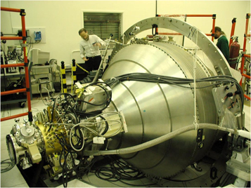
Figure 8. Assembled Dewar and Probe. Testing at Stanford in August 2002 shortly before shipment to Lockheed Martin Palo Alto Laboratory for integration with the Spacecraft.
Download figure:
Standard image High-resolution imageThe Dewar had several unusual features and one that was unique: a central cylindrical sealed section containing a 10−7 gauss 0.28 m diameter superconducting magnetic shield. The quantity conserved in a superconductor is magnetic flux (field x area). Cooling a folded lead bag through its superconducting transition and then expanding it lowers the field. The process, detailed in paper 9 [25], took three successive bags, each expanded in the reduced field of the previous one. Once this 0.28 m diameter low field region had been created, the Dewar was kept at or below 4.2 K for the entire four years of Probe development. That required a 1 m diameter, 3.8 m high 'airlock' (more exactly, helium lock) to allow insertion and removal of the warm Probe into and from the 4.2 K Dewar, a 24 h long procedure performed by a single team.
Liquid helium has very low latent heat  The refrigeration available in the gas on raising it from 2 K to GP-B's mean on-orbit skin temperature (255 K), was 61
 Circulating the gas through one or more shields in the Dewar could increase the hold-time by as much as a factor of 25. The Dewar had four shields, one more than prior flight dewars, thereby adding a further month to the life. The actual flight hold-time was 17 months 9 days as against the 16 month requirement. Another point (paper 11, [26]) was on orbit control of the fluid mass-center to avoid degrading the Spacecraft's pointing performance by helium slosh.
Figure 9 is the Probe, terminating in a 0.28 m long ambient temperature top hat containing valves, exhaust ports and electrical connections, plus a sunshade to prevent sunlight entering the telescope during the weeks around 11 March of closest alignment on the Sun. A shutter to be closed against heat from the Earth's albedo during the 'guidestar invalid' portion of the orbit is also indicated, but on-orbit it produced unacceptable vibrations and was far better left open. Resulting shifts in data were easily handled in the analysis.
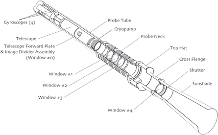
Figure 9. The 2.57 m long probe containing the Science Instrument Assembly was linked to the Dewar at five locations in the Probe neck. A 2.6 K cryopump maintained 10−14 Torr pressure. The sunshade shielded against incoming radiation including the Earth's albedo.
Download figure:
Standard image High-resolution imageTwo issues were first, to combine maximum transmission of guide star light with minimum heat input and second, the very exact design needed to allow repeated insertion and removal of the sealed Probe into the permanently cold ultra-low field region.
The Sun's heat load (reduced by covering the Dewar with FOSR8 flexible optical solar reflector) was 10 kW; the allowed input into the helium was 150 mW. The two necktubes, Dewar and Probe, had to be tied mechanically and thermally at four heat stations, bridged to the four vapor-cooled shields in the Dewar running at 24, 77, 110, and 190 K. Consider the top hat window and the thermal optical and microwave constraints on the Probe. Its surface area was ∼0.25 m2. At 255 K a black body of that area radiates 25 W, added to which was heat conducted down the elaborate system of pumping lines and coaxial leads of figure 10. The three lower Probe heat stations had 2° tilted fused silica windows, coated on their upper surfaces with a thin uniform layer highly reflective in the infra-red, with incoming microwave radiation attenuated by coating the outer surface of the top hat window with a proprietary (indium-tin-oxide) layer. The inner surface of the top hat and outer surfaces of the leads and pumping lines were gold plated. Five issues defining Probe layout were: ultra-clean, ultra-high vacuum, ultra-low magnetic field operation, gyro spin-up, and charge control.

Figure 10. Upper end of cryogenic Probe showing gold-coated leads and surfaces to reduce radiation and in lower left the first radiation window connected to the vapor-cooled shield.
Download figure:
Standard image High-resolution imageTo attain the low magnetic field for SQUID readout, the permeabilities and magnetic moments of every component in the cryogenic section were subject to severe constraints, individually checked before acceptance. Each screwdriver and wrench used in the assembly had to be custom-made from phosphor bronze rather than steel. Two further concerns were: (1) how to combine low on-orbit heat leak into the Dewar with rigid launch support, (2) how to avoid superfluid helium transfer at the launch pad. Concern 1 was met by using PODS Passive Orbital Disconnect Struts developed by Lockheed under a separate NASA contract to provide rigid support under tension or compression, relaxing in low-g. The actual gain was somewhat less than expected since 6 of the 12 PODS had to be shorted. For concern 2, avoiding superfluid transfer to a Spacecraft held with very restricted access in the Delta II vehicle chamber 125 ft above ground, the answer was a 'guard tank' mounted on the Dewar's 24 K heat-exchanger, filled once every 5 days with 4.2 K normal helium, the main tank being kept sealed for 60 days without going above 1.86 K.
A GP-B invention, used also in the IRAS, COBE, and European ISO infrared astronomy missions, was the superfluid porous plug. Ground-based dewars use gravity to separate gaseous and liquid helium; flight dewars need some other method. A porous plug at 1.86 K on the outlet of the main tank cooled the system by a method akin to sweating in a desert climate. The helium evaporates as it exits the plug and by fountain-effect cooling refrigerates the tank.
2.4. The 12 fundamental requirements
Twelve interconnected requirements shaped the building and management of GP-B:
- (1)Gyroscope drift-rate: the long-term nonrelativistic drift-rate referenced to inertial space was to be <0.3 marc-s yr−1 (1σ accuracy).
- (2)Detection and calibration: the overall drift-rate of each gyroscope with respect to IM Pegasi was to be measured with an uncertainty <0.3 marc-s yr−1, as calibrated from the annual and orbital aberration of the guide star.
- (3)Proper motion: the proper motion of IM Pegasi was to be determined in separate observations to a remote star to within 0.15 marc-s yr−1 in declination and right ascension.
- (4)Roll measurement and control: the rate and phase of Spacecraft roll about the line to IM Pegasi were to be measured and controlled to accuracies ensuring: (a) sufficient averaging of body-fixed torques; (b) resolution of the gyroscope drift rates in the NS and WE directions, each to <0.3 marc-s yr−1.
- (5)Gyroscope readout: the readout in the presence of a mean trapped field of 9 × 10⁻⁶ gauss, together with a single sided noise spectral density at the 77.5 s roll corresponding to a 1 marc-s readout resolution in 10 h.
- (6)Gyroscope spin-up and alignment: the rotors were to be spun to ∼100 Hz and aligned with the mean direction to IM Pegasi to within 10 arc-s.
- (7)Science telescope: the resolution error of the telescope and its readout within the ±60 marc-s readout range were to be <0.3 marc-s with a stability ∼0.1 marc-s.
- (8)Pointing: during the guidestar-valid phase of the orbit, total pointing error was to be <60 marc-s; during the guidestar-invalid phase pointing was to be kept within the reacquisition range of the telescope and pointing control systems.
- (9)Quartz block: the mechanical drift between each gyro readout and the telescope readout, referenced to inertial space was to be <0.1 marc-s yr−1.
- (10)Bias rejection: the joint effect of all the bias drifts, electronic, magnetic, optical, thermal, and mechanical on the gyroscope readout, telescope readout, science data instrumentation system, and data reducing system with respect to inertial space was to be <0.1 marc-s yr−1.
- (11)Telemetry and data processing: the science gyroscope and telescope signals (SG, ST)were to be conditioned, sampled and processed so that they could be differenced on the ground with no added telemetry/data processing error >0.1 marc-s. All science signals were to be synchronized and time tagged to GPS time to <0.1 ms. A science data reduction system would determine the relativity terms from the telemetered SG, ST, roll, tracking, and time data.
- (12)Validation: in addition to the net common result from all four gyroscopes the experiment validity was to be checked by auxiliary tests in which potential disturbances on the gyroscopes and other instrumentation were deliberately enhanced. Cross checks would include comparison with known results from the relativistic bending of starlight, stellar parallax, the distance to the guide star, and the geodetic measurement itself.
Defined in 1986, the 12 requirements linked coherent goals with adjustment as hardware developed. Take the 60 marc-s pointing of requirement 7, considered extreme in 1960. The first thought was to add fine-pointing cryogenic actuators. Actually, with continuous gas flow and proportional thrusters GP-B achieved 20 marc-s, but there was more at stake. Consider requirement 8, which had two parts—'guidestar valid' and 'guidestar invalid'. During 'invalid' with IM Pegasi hidden behind the Earth, the gyro readouts provided the reference. The issue was not 60 marc-s pointing but reacquiring IM Pegasi on entering 'guidestar valid'. During the first two months of Science, August through September 2004, reacquisition took 20 min; more sophisticated tracking reduced this to 1 to 2 min.
3. Spacecraft, attitude-translational control (ATC), and mission operations
3.1. Spacecraft
Figure 11 is the Spacecraft. Its main structural element was the Dewar, on to which was bolted a welded aluminum truss carrying batteries, Sun sensors, payload electronics, GPS antennae etc, and four hinged solar arrays unfolded during ascent to the on-orbit configuration. The arrays were double-sided with 22° tilt, optimized to IM Pegasi's 16.8° declination. The net mean power over the year was 500 W. Power when the Sun was eclipsed came from two 35 A-hr super Ni–Cd batteries. A NASA Standard Power Regulator Unit controlled power to the batteries and all onboard electronics.
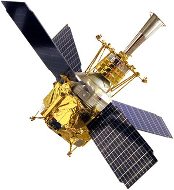
Figure 11. Spacecraft. The 5 m long 1.6 m diameter Spacecraft has four tilted solar arrays oriented to provide optimum mean power through the year, two tilted clockwise and two counterclockwise to balance torques from residual air and solar radiation pressure.
Download figure:
Standard image High-resolution imagePaper 12 [27] reviews the many Spacecraft systems: (1) command and data handling (2) electrical power (3) thermal control (4) ATC (5) communications, (6) payload electronics, and three mechanisms: a GMA for gyro spin-up, an attitude reference platform for roll, and a mass trim mechanism to bring the Spacecraft axis into close coincidence with the SIA. A further essential function of the GMA was 'trapped flux reduction'. Launch vibration drove the rotors' niobium coatings to the normal, non-superconducting state. A two day flux reduction at 10 K in the Dewar's ultra-low field bag restored the required 9 × 10⁻⁶ gauss level. Other on-orbit matters were: minimizing aerodynamic, magnetic, and eddy current effects on the vehicle, isolation of the payload electronic boxes, saving lost communication by having two transmission systems: A-side and B-side.
3.2. Attitude-translational control
The Dewar boiloff gas vented continuously through proportional thrusters gave far smoother control than standard 1960s pulse-width pulse-frequency or bang–bang systems. With air drag and solar radiation pressure about equal at 642 km altitude; going higher would have gained little and going lower would have rapidly raised the drag to a level beyond the available thrust. Three key numbers were: first Dewar boiloff rate (7.4 mg s−1), next the very low Reynolds number (Re = 10) of the flow rate in each nozzle, and third the specific impulse Isp (figure 12(a)) which determines the thrust for a given flow. Studies by Bull (1972) utilizing a laboratory test stand with sub-dyne resolution to measure thrust versus flow rate showed that the Isp of the helium exiting an actual nozzle was 130 s close to the ideal expectation.

Figure 12. Stanford laboratory data on helium specific impulse (a) as function of mass flow rate; sectioned view (b) of the Lockheed Martin proportional flight thruster.
Download figure:
Standard image High-resolution imageFollowing initial Stanford research, flight thrusters (paper 16, [30]) were developed and tested at Lockheed Martin utilizing, wherever possible, known flight hardware. Figure 12(b) is a sectioned thruster controlled through a teflon-capped titanium piston supported by two stainless steel springs, with the nozzle's expansion ratios and half angles chosen to optimize Isp. Through the throat the gas flowed like honey; at the nozzle it went sonic. The required rate was 4.1 mg s−1; the Dewar boiloff was 7.4 mg s−1; a piezoelectric transducer controlled the flow. The final layout had 16 thrusters, in four 4-way sets. While two years of ground testing had established their reliability well beyond the expected range, two, #6 aft and #8 forward, both in the same translation plane failed, during on-orbit set-up and had to be closed off. The remaining 14 maintained a stable operation: roll frequency 12.9 mHz within 0.13 mrad, while holding inertial pointing to within 20 marc-s, well below the 60 marc-s of requirement 7.
As for the number of thrusters, DeBra in an early investigation showed that for GP-B's six degrees of freedom system (three translational, three pointing) seven thrusters arranged non-orthogonally would meet the need. Having 16 thrusters assured good on-orbit redundancy.
3.3. Mission operations
The GP-B MOC, seen in figure 13, was set up on the Stanford campus, greatly easing Science operations. Having the MOC on campus made for close communication between NASA, the Science team, and newly arrived MOC personnel. A separate room adjacent to the MOC for daily planning meetings further aided the process. Communication between the Spacecraft and MOC was by two means: first a 2 kilobit s−1 Space network link primarily for mission set up, carrying real time commands up to the vehicle and real time engineering data down to the MOC; second, a 32 kilobit s−1 network delivered the science data and allowed commands to be uploaded for autonomous implementation. Central was a Spacecraft computer to collect data and receive commands, which communicated with a second on-board computer controlling the SQUIDs, the telescope and four suspension system computers, one for each gyroscope.

Figure 13. The GP-B Missions Operations Center in a specially constructed building located on the Stanford near-West campus.
Download figure:
Standard image High-resolution image4. Data analysis: science data, models, results
The science data covered 352 days, 28 August 2004 to 15 August 2005, with nine interruptions due to loss of guide star pointing, leading to ten distinct data segments. Most dramatic was the disruption on 20 January 2005 by an X-class solar flare. Three other events during March 2005 arose when it became necessary to switch the output from the 'A-side' computer system to the backup 'B-side', with a detailed operating recalibration.
Obtaining the data and comparing it with GR took four signals, linked and matched to 0.1 ms by methods described in paper 14 [28]: (1) four SQUID readouts, one for each gyroscope; (2) the X- and Y-axis telescope readouts from four pairs of 72 K Si-photodiodes; (3) roll phase data from the attitude reference platform; (4) GPS orbit data to compute the effects. Good subtraction of the gyroscope and telescope signals required matching the two scale factors, AG and AT, to ∼0.5%, performed in ground based analysis by injecting a 30 marc oscillation of known frequency into the pointing signal and driving [AG (ωd) − AT (ωd)] to zero. Different dither periods were used for the two telescope axes, initially 30 s for X and 40 s for Y. Given the danger of the 40 s dither being too close to the second harmonic of the Spacecraft's 77.5 s roll, we changed them on 16 December 2004 to 29 s and 34 s. For details see paper 18 [32] (DA I).
The two data analysis methods mentioned earlier, Algebraic and Geometric, came from the fact that the largest of the disturbing torques on the gyroscopes was the misalignment term shown in figure 17. See papers 18, 19, and 20 [32–34].
4.1. Science data
The raw outputs from the SQUIDs, telescope, and other flight hardware, were processed by on-board computers and telemetered to the MOC. The SQUIDs tracked gyro drift; the telescope measured Spacecraft pointing, and the attitude reference platform star trackers and rate gyros gave roll phase. The GPS data served two functions: (1) tracking the exact positon and velocity of the Spacecraft to obtain the calibrating orbital aberration profiles of the gyroscope scale factors; (2) precise calculation of the predicted Ωfd Ωg.
Gyro readout. Sampled at 2200 Hz by a multiplexed 16 bit A/D converter, the SQUID signal was recorded in two channels: a high bandwidth one for signals at harmonics of the gyroscope spin rate for flux mapping, and a low bandwidth channel for Spacecraft roll data. The high bandwidth signals passed through a 780 Hz analog low pass filter before sampling by the A/D converter; snapshots of 4096 continuous points were collected and processed. The digital data were processed on board using a fast Fourier transform algorithm, with frequency bins surrounding the first five harmonics of each gyroscope's spin speed, real and imaginary parts of the signal being included in the telemetry. The low bandwidth channel passed through an additional analog low pass filter with 4 Hz cutoff, attenuating the gyro spin signal, reducing its peak-to-peak trapped flux amplitude. This filtered signal was amplified before A/D sampling, then processed using a digital Kaiser non-causal low pass filter with 2.5 Hz cutoff, 2200 overlapping points being filtered every 0.2 s to give a single datum. Snapshots with 4096 points of the 2200 Hz low bandwidth digital data were occasionally collected.
Telescope readout. Two Si-photodiodes in charge feedback loops sampled at 2200 Hz, reset every 0.1 s, formed the telescope readout. An on-board Kalman filter determined the photocurrent from the rate of change of the loop output, with telescope pointing calculated from these currents, and snapshots of the 2200 Hz digital signal available as a crosscheck.
Roll phase. The Spacecraft roll phase was calculated every 0.1 s in an Earth-centered, inertially-fixed reference frame using the star tracker and rate gyro data from one attitude reference platform, directly available also on the ground for roll phase refinement.
GPS receiver. Every 10 s a GPS receiver provided GPS time and the position and velocity of the Spacecraft for the exact orbit determination described in paper 17 [31].
Timing. A 16 MHz oven-controlled crystal oscillator, from which came a 10 Hz data strobe in each 0.1 s interval, provided the on-board timing to link the four signals. In total, 128 bytes of information comprising the science data record were stored with vehicle time. Snapshots were labeled at their midpoint, duly corrected on the ground for data latency that resulted from on-board filtering and processing. The data were not recorded at one uniform rate, nor were all points available at each discrete instant. For these reasons and to reduce the computational burden in Ωfd, Ωg analysis, the data were processed on the ground to one datum per every 2 s.
4.2. Analysis models
The analysis advanced in three stages: (1) pre-launch studies; (2) initial results; (3) advanced post-launch analysis, in which the three surprises of section 1.3, polhode damping, misalignment torque and roll polhode resonance, were computed and resolved.
4.2.1. Pre-launch
Kalman filter studies of modeled GP-B data were performed in the 1980s by Breakwell, Vassar, and Duhamel. Topics included: (1) London moment readout scaling against orbital aberration; (2) Spacecraft pointing and gyro/telescope scale factor matching; (3) data interruptions, long and short; (4) use of the rotor's residual trapped flux to improve AG calibration; (5) the time evolution of the combined Ωfd, Ωg and annual aberration data for missions with different inclinations and start dates. A noteworthy finding was that an optimally launched GP-B, in an 86° co-inclination orbit, would have 30% better Ωfd accuracy than a polar orbit—but the case for a polar orbit remained compelling. Breakwell, Vassar, and Duhamel's predicted experiment accuracy was ∼0.5 mas yr−1. Further pre-launch investigations included a succession of detailed end-to-end data reduction tests carried out by Keiser et al [16] from 1996 on developing the required on-orbit software to process the actual flight data, which was to prove essential in overcoming the three surprises.
4.2.2. Initial results
Figure 14 is one half-orbit of SQUID data as the Spacecraft rolled about the line to IM Pegasi. Superimposed on the 77.5 s roll signal is the orbital aberration, reaching 5.186 arc-s with the Spacecraft at the equator, vanishing over the poles. Figure 15 shows the four gyroscopes' North–South drift profiles from preliminary analysis of the science data. The ∼6.6 arc-s yr−1 Ωg effect is instantly visible; in a Newtonian universe they would have been horizontal lines. The lines are not perfectly straight: other effects were present, and in the East–West Ωfd profiles dominant. Analysis required treatment of the three surprises, now understood to originate in torques due to coupling between patch potentials on the rotor and housing.

Figure 14. One half orbit of SQUID readout data, showing how the 5.186 arc-s orbital aberration of the light from IM Pegasi calibrates the gyroscope scale factor AG.
Download figure:
Standard image High-resolution image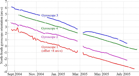
Figure 15. North–South drift profiles for the four gyroscopes, with processing based upon pre-launch considerations. The data gaps were caused by Spacecraft operational issues. Looking at the raw data we can see relativity.
Download figure:
Standard image High-resolution imageSurprise 1: polhode damping. Prior to launch we had expected the rotors' polhode motions to be closed paths with fixed periods. Instead (figure 16) the periods changed with time; in two cases (Gyros #1 and #2) even increasing for a while before reaching final steady rates after 30–70 days. This evolving polhode rate, and with it the changing angle between the spin and angular momentum axes, modulated the coupling of the rotor's trapped magnetic flux to the pick-up loop, making the gyroscope scale factor vary, besides causing an apparent time variation of gyro torques, even though the evolution was not the result of a torque.
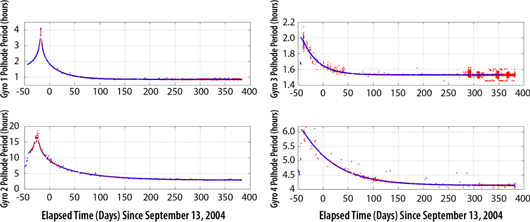
Figure 16. Changing polhode period profiles for the four gyroscopes, showing final convergence on constant periods after damping times ranging from 30 to 70 days.
Download figure:
Standard image High-resolution imageSurprise 2: misalignment torque. Next in figure 17 is data from Gyro #3 revealing during post science calibration, a gyroscope torque ∼1000× higher than expected when the misalignment angle τ(t) was increased during post science calibration by pointing the Spacecraft to stars 0.4°–7° away from IM Pegasi. For τ(t) <1°, the drift rate (different for each gyroscope) was ∼1 arc-s/day/degree. Changing from ac to dc support with τ(t) held constant, brought a further increase, and this, along with the separate analytical and experimental evidence presented in section 4.3.2 traced all three surprises to patch effect coupling. In 2009 Keiser et al [17] calculated the resultant torque by expanding fixed patch potentials on the rotor and housing in spherical harmonics, solving Laplace's equation to find the field between them, and then computing the energy stored in the field. The calculated torque, expressed with respect to the two Euler angles defining the spin axis orientation, was in impressively good agreement with the observed misalignment torque.
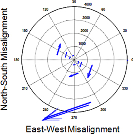
Figure 17. Misalignment torque for Gyro #3: a polar plot with zero misalignment at the origin. Each arrow represents a single post science calibration test, with the Spacecraft pointed away from the guide star. The location of each arrow's tail is given by the amplitude and direction of misalignment; arrow length represents the observed spin axis drift-rate.
Download figure:
Standard image High-resolution imageSurprise 3: roll-polhode resonance. The greatest surprise, seen in figure 18 was that all four gyroscopes followed smooth drift paths, then one (in this case Gyro #2) would rapidly step over by 20–100 marc-s in less than a day to a new direction, where it again settled down. The point at which the steps occurred was always when some very high harmonic of the slowly changing polhode period came into resonance with Spacecraft roll. The successive steps from May through July 2005 in the data for Gyro #2 were at the 146th, 145th,...., 138th harmonics. Results ranged from three such steps for Gyro #3 to more than 200 for Gyro #2.
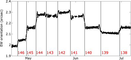
Figure 18. Spin axis profile for Gyro #2, highlighting orientation steps due to roll-polhode resonance torque. The numbers at the bottom are the values of the harmonic of the ever-changing polhode frequency that equal roll frequency at the indicated time.
Download figure:
Standard image High-resolution imageThese roll polhode resonances also originate in patch effect torques, depending on just two parameters, the distribution of patch potentials on the rotors and housing. Figure 19(a) is the calculated path of the spin axis around the resonance, a Cornu spiral; 19(b) is the observed path of Gyro #2 when the 277th harmonic of the polhode frequency resonated with Spacecraft roll, each point being the average orientation of the gyroscope spin axis during one 'guide star valid' period. Within the estimated error, the agreement between the observed path and the calculated spiral is excellent.
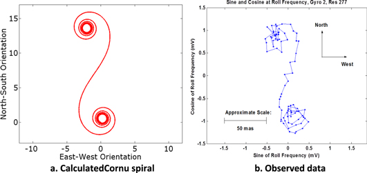
Figure 19. Theoretical and experimental paths of the roll polhode resonance transition.
Download figure:
Standard image High-resolution imageStudies by Buchman and Turneaure [18] of 50–100 mV patch charges on the rotor and housing surfaces defined the underling physics. Pre-launch micrographs had indicated a polycrystalline surface morphology with 0.1–1 μm length-scale, which if reflective of patch potential scale would have given negligible torque. Following launch, additional laboratory measurements on a flight-like rotor demonstrated a patch potential scales ranging from 0.1 to ∼50 mm. This, combined with the assumption of a similar length-scale for housing potentials, provided the physical description needed to understand and model these surprise torques on the GP-B gyroscope. The Buchman–Turneaure model also gave predictions of three additional on-orbit effects: (1) a steady acceleration of the gyroscope along its roll axis, (2) a periodic acceleration at its spin frequency, (3) a computation of the gyro spin down rate.
4.3. Model extensions
The surprise torques and polhode damping called for more refined data modeling. We start with readout considerations.
4.3.1. Readout scale factor
The SQUID readout had two terms: the London moment ML aligned with the gyroscope spin axis, and trapped flux in the rotor body. Polhode damping made the trapped flux move relative to ML as seen for Gyro #1 in figure 20, with similar results for Gyros #2, #3 and #4. The resulting SQUID scale factor had three elements CLM (London moment), CTF (trapped flux), CE (electronics), with CTF ∼1% of CLM, and CE a 0.1% adjustment to CLM to account for electronics variations. CLM was constant up to the rotors' very small (∼10−4 yr−1) spin-down rates. CTF was found by the 'trapped flux mapping' process described in papers 6 [23] and 19 [33], with the rotor motion and trapped field distribution estimated by fitting to spin harmonics of the SQUID's trapped flux signal yielding: (1) a history of the polhode phase for each gyroscope to 1° throughout the mission (2) CTF, accurate relative to CLM to ∼10−4. Its time signature came from that portion of the polhode-modulated trapped field parallel to the gyro spin axis.
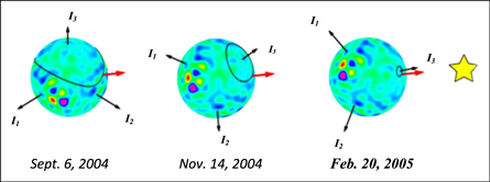
Figure 20. Trapped flux map for Gyro #1 on 6 September 2004, 14 November 2004, and 20 February 2005. The color pattern depicts the variation in trapped magnetic flux across its surface. The three views reveal dissipation-induced polhode damping toward the principal moment of inertia. The red arrow denotes the rotor's spin axis.
Download figure:
Standard image High-resolution image4.3.2. Gyro dynamics
Essential to determining Ωg, Ωfd in the presence of the surprise torques was to include the physically justified misalignment and roll polhode resonance terms in the defining equations for the drift rates for the gyroscope spin axis in the North–South and East–West directions
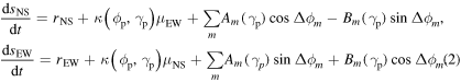
The North–South, East–West drift rates dSNS/dt and dSEW/dt are each a sum of three terms: (1) the relativistic drifts rNS, rEW of the gyroscope's spin axis orientation, yielding Ωg, Ωfd; (2) the North–South, East–West terms k(ϕp,γp)μEW and k(ϕp,γp)μNS arising from misalignment torques; and (3) sums defining the roll-polhode resonance torques where Am(γp) and Bm(γp) multiply the sine and cosine differences between the Spacecraft roll phase ϕroll and the mth harmonic of polhode phase ϕp. See section 2.2.3 of paper DA I [32].
Two expansions, one for the rotor, one for the housing, fixed in their respective frames defined the patch potential distributions. Transformed to the housing frame, taking spin and polhoding into account, these gave the energy stored in the field in terms of angles defining the gyro spin axis orientation and the amplitudes and phases of the spherical harmonic expansions by calculating the change in stored energy for a small change in spin orientation. Averaging over roll gave the misalignment torque; the result without averaging gave the roll polhode resonance torque. The net result was a parametrization in terms of the physically meaningful k(ϕp,γp), Am(γP), Bm(γP) and Δϕm seen in equation (2). Details are in appendix C of paper DA I [32].
Stated in the simplest terms while the presence of the electric patch charges was a complication for Gravity Probe B, the parallel effect of the non-uniform magnetic trapped flux was a help, it caused no significant torque but provided the necessary mapping for us to deal with the parch torques.
4.4. Estimation tools
The drift rates and torque coefficients were determined by fitting the science data to equation (1) using '2-second filter' software (so named because the science data comprised one datum every 2 s). The filter was a modular, scalable nonlinear least-square Bayesian estimator, capable of fitting the ∼107 point data set for each gyro to the much smaller number of gyroscope parameters (∼100–1000). The estimator was nonlinear because of the presence of sinusoidal terms in equation (2). The number of model parameters was easily adjusted to study modeling sensitivity. The filter used guidestar valid data; separate software tracked the torque-induced gyro drift during the guidestar invalid phase.
The filter, an iterative algorithm based on the linearization of the measurement model about the current state vector estimate for each parameter in the model, to give the Jacobian matrix and corresponding covariance matrix. The Jacobian was determined analytically. Next, we calculated measurement residuals (and associated corrections). The resulting state vector estimate and covariance matrix led to an updated estimate. A separate preliminary analysis provided the good initial state vector necessary to find the correct final state vector estimates for this nonlinear system. The computation was an intensive process using the 44 parallel processors of the Stanford University ME NIVATION and REGELATION cluster, with an additional 12 Linux computers set up in HEPL (the Stanford University Hansen Experimental Physics Laboratory). The filter typically converged after ∼20–30 iterations as the state vector corrections became sufficiently small.
5. Results
The science data had ten segments, of which the 2 s analysis used six. Segment 1 was excluded because of inadequate pointing data; three others were too short (∼1 week or less) to count. To increase reliability, and bring improved understanding of the underlying physics, we obtained results in multiple ways, focusing first on Ωg, Ωfd. Consistent values for other model parameters further increased the reliability of the estimates. The four gyroscopes were analyzed independently, utilizing all six segments in a single fit. The Ωg, Ωfd estimates were then combined to produce a single result. Table 1 (section 1.4) gives the individual and joint results, also plotted as 95% confidence ellipses in figure 21.
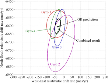
Figure 21. North–South and West–East uniform drift-rate estimates for the four individual gyroscopes (colored ellipses) and the combined estimate (black ellipse).
Download figure:
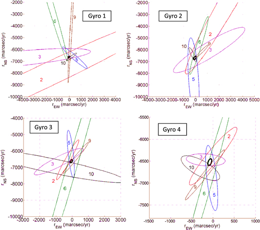
Standard image High-resolution imageFurther confirmation came from analyzing the six segments for each gyroscope separately, producing 24 independent estimates for Ωg, Ωfd. Figure 22 shows the resulting drift-rate estimates and 95% confidence intervals for the 24 individual gyro-segment runs. Not all 95% confidence ellipses were expected to overlap but all 24 estimates are consistent within their respective 95% confidence intervals. The size and orientation of each ellipse depended on the length and time of year of the segment. The length of a given segment defined the amount of data; longer segments yielded smaller uncertainties. The orientations of each ellipse result from the uncertainty introduced by the misalignment torque. This torque, acting in the preferred direction perpendicular to the gyro misalignment, caused increased uncertainty in this time-varying direction.
Figure 22. North–South and West–East relativistic drift-rate estimates for all 24 gyro-segments analyzed independently.
Download figure:
Standard image High-resolution image
The end-estimates were weighted means of ten individual ones, computed using ten distinct sets of parameters for each gyroscope. The models for scale factor Cg(t), polhode phase ϕp(t), misalignment torque coefficient k(t), and Spacecraft pointing τ(t) were sums of particular basis functions. The number of terms used in each was increased from one until the change in the rNS, rEW estimates from the defining equation became <0.5σ. The table 1 results were weighted means of the baseline run for each gyroscope plus nine 'sensitivity runs', in each of which the number of terms in one of the models was raised by one above the baseline value (paper 18, [32], sections 4–7). Table 2 gives the number of parameters and the amount of data for each gyroscope. The number of parameters largely depended on the number of roll-polhode resonances, each of which required two model parameters. Only ∼25% of the parameters had a correlation >0.1 with respect to the Ωg, Ωfd rates, even though all were required to explain the data to the SQUID noise limit. The χ2 per degree of freedom of the post-fit residuals of the 2 s filter was ∼1 for all gyroscopes.
Table 2. Number of parameters and days of data analyzed per gyroscope.
| Source | No. parameters | No. days of data |
|---|---|---|
| Gyroscope 1 | 154 | 200.7 |
| Gyroscope 2 | 662 | 219.7 |
| Gyroscope 3 | 139 | 188.8 |
| Gyroscope 4 | 272 | 241.7 |
| All Gyroscopes | 1227 | 850.9 |
Note: the 'days of data' are in five or more sets spaced throughout the mission.
The uncertainties in figure 21 include both statistical and systematic effects, listed separately in table 3, where two classes of systematic error are listed. The first class of systematic uncertainty is small effects not present in the model, such as unmodeled torques, telescope and gyroscope readout, and guide star proper motion. Papers 6 [23] and 8 [24] review the telescope and SQUID readout; paper 21 [35] reviews the uncertainty in guide star proper motion. 'Other nonrelativistic torques' in table 3 includes the mass unbalance and suspension effects discussed earlier and various parameters determined on the ground and on-orbit. The second class of systematic uncertainty quantifies the sensitivity to the number of model parameters. The combined baseline + 9 sensitivity runs for each gyroscope produced 104 four-gyroscope estimates when all possible individual combinations were computed. The covariance of these 104 estimates was the systematic uncertainty associated with parameter sensitivity shown in table 3.
Table 3. Contributions to experiment uncertainty.
| Contribution | NS (mas yr−1) | EW (mas yr−1) |
|---|---|---|
| Statistical (modeled) | 16.8 | 5.9 |
| Systematic (unmodeled) | ||
| Parameter sensitivity | 7.1 | 4.0 |
| Guide star motion | 0.1 | 0.1 |
| Solar geodetic effect | 0.3 | 0.6 |
| Telescope readout | 0.5 | 0.5 |
| Other readout uncertainties | <1 | <1 |
| Other nonrelativistic torques | <0.3 | <0.4 |
| Total statistical + systematic | 18.3 | 7.2 |
The final four-gyroscope result was computed by first combining the four individual gyroscope estimates, using their statistical covariances, and accounting for any over/under-dispersion of the individual estimates. The resulting statistical uncertainty was then added in quadrature to the systematic ones to produce the overall uncertainty shown in both tables 1 and 3.
The misalignment torque of figure 17 caused a drift predominantly orthogonal to the misalignment plane. The alternative 'geometric method' of handling the data, mentioned earlier, exploited this orthogonality. By analyzing the drift-rate in a direction parallel to the misalignment, the need to model the misalignment torque was eliminated. Also different ways of modeling the resonance torques became possible, either by using two parameters and the known phase difference for each resonance, or by omitting data close to each resonance. The result, using two data segments from Gyro #2 and four from Gyro #4, was −6,676 ± 31 mas yr−1 in the North–South direction and −48 ± 26 mas yr−1 in the East–West direction, consistent to ∼2σ with GR, in strong confirmation of the results from the algebraic method. A further cross-check was that the geometric method gave an independent estimate of the gravitational deflection by the Sun of the light from IM Pegasi, consistent with the GR prediction to within 20%.
6. Conclusion
Through a combination of space technology, cryogenics, and high-precision engineering, Gravity Probe B measured two untested effects of Einstein's theory of gravitation, GR: the geodetic and frame-dragging precessions of gyroscopes in Earth orbit. The predicted GR values in GP-B's 642 km polar orbit were for frame-dragging—39.2 marc-s yr−1 and for the geodetic effect—6606.1 marc-s yr−1. The measured one sigma results were frame-dragging—37.2 ± 7.2 marc-s yr−1 and geodetic—6601.8 ± 18.3 marc-s yr−1. The accompanying 20 papers in this CQG issue detail the many technologies and data analysis techniques of the mission.
Acknowledgments
Gravity Probe B was the result of collaboration between Stanford University, NASA George C Marshall Space Flight Center, and Lockheed Martin with other academic and industrial partners noted in the text. The program is under great obligation to the NASA appointed Science Advisory Committee chaired by C M Will. Other key advisors over the years include: Rai Weiss, Israel Taback, Parker Stafford, Charles Pellerin, Jeffrey Rosendhal, and Graham Siddall. Deceased contributors include: William Fairbank, Donald Davidson, Richard Potter, Joyce Neighbors, and Wilhelm Angele. The Gravity Probe B staff at Stanford and NASA Marshall Center comprised of around 150 persons, in total there were 330 students on the Mission including 84 who were awarded Stanford doctorates and 16 doctorates at other universities in the US and abroad.
Footnotes
- 7
Southwood's reversal technique allowed roundness measurements accurate to <0.1 μin from a spindle with ~0.5 μin out-of-roundness by combining successive measurements on a GP-B rotor with the rotor turned 180°.
- 8
Invented in Japan in 1986 by Yoshinori Hasuda, Shigekuni Sasaki, and Toshihiro Ichino.