


Abstract
Frequently, in university-level general physics courses, after explaining the theory, exercises are set based on examples that illustrate the application of concepts and laws. Traditionally formulated numerical exercises are usually solved by the teacher and students through direct replacement of data in formulae. It is our contention that such strategies can lead to the superficial and erroneous resolution of such exercises. In this paper, we provide an example that illustrates that students tend to solve problems in a superficial manner, without applying fundamental problem-solving strategies such as qualitative analysis, hypothesis-forming and analysis of results, which prevents them from arriving at a correct solution. We provide evidence of the complexity of an a priori simple exercise in physics, although the theory involved may seem elementary at first sight. Our aim is to stimulate reflection among instructors to follow these results when using examples and solving exercises with students.
Export citation and abstract BibTeX RIS
1. Introduction
In daily life and in their professional activities, people dedicate much intellectual effort to solving problems. Because of the centrality of problem-solving to work and everyday life, problem-solving should also be central to education. In 2007, the Tuning Project [1] conducted a survey amongst physics academics across Europe (one physics department for each EU country) and employers of physics graduates. One of the results identified the ability to identify, formulate, and solve physics problems as essential outcomes of any physics program. It is a common assumption in physics education that solving problems leads to understanding of the subject and that it is a reliable strategy to test the learning achieved by students [2]. However, research has repeatedly shown that many students following general physics courses at university in traditional teaching formats learn to solve different types of quantitative exercises that feature at the end of each textbook chapter but are usually unable to explain the meaning of their own numerical solutions to the problems [3, 4].
Previous studies on physics problem-solving show the restrictions of traditional teaching of problem-solving among students. University students typically use mathematics and formulae as the first step in solving problems, which is hardly surprising since their instruction is widely focused on content of this kind. Even after they have solved a wide variety of problems, however, it has been found that the most common 'alternative conceptions' detected by physics education research (PER) remain intact [5]. Traditional instruction in physics courses focused on problem-solving usually leads to poor achievement in terms of developing skills and procedures associated with problem-solving [6].
In order to help students solve problems, other types of teaching strategies have been developed which are predicated on the assumption that comprehensive learning and problem-solving is achieved by acquiring scientific abilities that are needed to formulate solving strategies and to construct explanatory models [7, 8]. These proposals suggest that instructors should not just explain the problem's numerical resolution but also utilize a teaching strategy that gives students the opportunity to use scientific procedures such as putting forward a hypothesis about the relevance of a model to the problem proposed, suggesting a number of different strategies to explain it, and justifying the answer based on evidence [9].
The research on problem-solving has focused on problems such as those listed at the end of the chapters of textbooks or complex problems that do not have a single correct answer [2]. However, in this study, we focus on the solving of seemingly simple exercises by university-level students and instructors which are used to illustrate concepts and laws in textbooks. What we are suggesting is that even exercises that set out to apply theory directly must follow the recommendations made by researchers on problem-solving if they do not want students to fall victim to misconceptions. Firstly, we provide evidence of the complexity of an a priori simple exercise in physics, although the theory involved may seem elementary at first sight. Secondly, we discuss the solution to the problem following the recommendations of problem-solving research.
2. Study
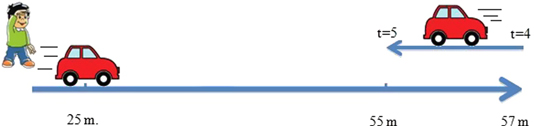
To present an example that is commonly used to illustrate theory, we designed one paper-and-pencil problem. The exercise selected is one often set at high school level (16–18 years old) and introductory physics courses at university level. Therefore, it was decided to choose a problem of kinematics in one dimension, which usually appears in the first chapters of a physics course. The aim was to find classroom problems that would be familiar to students at these levels and on which the students would receive instruction in any case, regardless of the educational demands of the school or college. We did not want to select a problem on a topic in the syllabus that might be covered in a quick way due to lack of time, or which would place heavy cognitive demands on learners. This is exercise #1 (see figure 1).
The study was carried out with 1396 students and instructors from the Basque Country (Spain) during the last three years, including 715 high school students from (16–18 years old), 593 students from first-year undergraduate engineering at the University of the Basque Country and 88 undergraduate science instructors (physics, chemistry, life sciences and mathematics) were asked to solve the problem. The high school and university students tackled the problem after receiving classes on kinematics and under examination conditions. The mark awarded for solving the problem was part of the final assessment. High school students had completed at least one year of physics (4 h per week), which involved the topic 'Motion in one dimension'. First-year engineering students had received 3.5 h of lectures and 2 h in the lab per month for 14 weeks on mechanics. The chapter 'Motion in one dimension' is taught for two and a half weeks of this course.
The instructors were assistant lecturers. The instructors were asked to attempt the problem during a training course on teaching science problem-solving organized by the University of the Basque Country as part of the professional development program for teaching faculty.
3. Results
We are aware that problem-solving is a complex process in which it is hard to separate the different aspects of procedural knowledge and so a continual interaction between the different stages is necessary. For this reason, we first present the solutions obtained by the students and teachers (see table 1) and then discuss the steps that they went through to arrive at their solutions.
Table 1. Results of exercise #1: the total distance travelled by the car in 5 s.
| Answers in percentages | ||||
|---|---|---|---|---|
| Sample | Correct | 55 m | 30 m | Others |
| High school (715) | 0.0% | 70.0% | 15.0% | 15.0% |
| Year 1 engineering (593) | 0.0% | 47.0% | 43.0% | 10.0% |
| Instructors (88) | 4.5% | 21.5% | 72.0% | 2.0% |
What could be the reason for such a widespread wrong answer? The errors made by students and instructors on the 'exercise' can be interpreted in terms of several distinct tendencies in reasoning.
The most common incorrect response to the problem made by the vast majority of high school (HS) students (70%) and almost the majority of university students (47%), is that they directly replace the data in the equation to obtain the result equal to 55 m. The following explanations were typical.
'The equation provides the travelled distance over time. Therefore, at 5 s, the vehicle has covered the following distance: s = 25 + 16*5 − 2*25 = 55 m' (high school student).
'The equation shows the distance covered by the car over time. Substituting into the equation t = 5 s a distance of 55 m is obtained' (university student).
A minority of HS student responses (150 of 501) and more than half of university students (190 of 279) who answered s = 55 m, added explanations concerning the kinematics of movement. We believe that this explanation about the physics of the problem does not represent a distinct strategy of solving the problem. However, it almost certainly reflects the emphasis on exercise-solving methods in teaching about kinematics. Examples of responses phrased in terms of the physical meaning of the equation, are the following.
'The equation shows movement in a straight line with constant negative acceleration. Therefore, at 5 s, the vehicle has covered the following distance: d = 25 + 16*5 − 2*25 = 55 m' (HS student).
'The equation represents the distance of a rectilinear movement with uniform deceleration over time. At 5 s, the distance covered is: d = 55 m' (university student).
In their response to the problem, a minority of HS students (15%) and less than half of the university students (43%) claimed that the existence of 25 m of initial distance between the car and the reference point would mean that the travelled distance is 30 m, as in the following explanations.
'The equation represents a motion with negative constant acceleration. At 5 s, the distance covered is: d = 55 m. As there is an initial distance of 25 m, the car has covered 30 m' (university student).
'The equation x = x0 + v0t + 1/2at2 represents a uniformly accelerated motion in one dimension. If we can compare the equation of the exercise with the general equation, we calculate that for t = 5 is x = 55, but the initial distance is 25, so the total distance travelled is 30 m' (instructor).
As for the instructors, the characteristic feature of their responses (72%) is that they begin by processing the information directly within the framework of an identifiable model, and then they use the data supplied in the equation. For example:
'The equation x = x0 + v0t + 1/2at2 represents a uniformly accelerated motion in one dimension. If we can compare the equation of the exercise with the general equation, we calculate that for t = 5, x = 55, but the initial distance is 25 m, so the total distance travelled is 30 m' (instructor).
A minority of instructors (21.5%) that used the above strategy did not take into account the initial distance, and they calculated the total distance as 55 m.

Figure 1. Exercise #1. English version of a problem of constant acceleration in one dimension.
Download figure:
Standard image High-resolution imageFew answers use the space/time graphic to obtain the result. In the case of students, no HS student used a strategy involving graphs to solve the problem. This may be because, although they studied the s/t and v/t graphics in the chapter on kinematics, in traditional Spanish teaching almost all the exercises of the kind we present here are taught using the strategy of equations of motion. Of the six university students that solved the problem by developing an s/t graphic, not one calculated the correct result, although they drew the s/t graphic correctly (see figure 2). For example:
'The graphic s/t shows that the car has a parabolic movement and the distance is the difference between the s coordinate at t = 0 and at t = 5, so the result is s = 30 m'

Figure 2. s/t graph for second 0 to second 5.
Download figure:
Standard image High-resolution imageOnly four instructors (all of whom taught mathematics) calculated the correct result. They solved the problem using a space/time graphic representation of the equation (see figure 2) and then calculated the corresponding coordinates. For example:
'The equation represents a parabola in the graphic s/t (see figure 2). The parabola has a maximum in t = 4 s and then descends. Therefore, you have to calculate the coordinate s between t = 0 s and t = 4 s: the value is s = 57 − 25 = 32 m. We also have to calculate the coordinate s between t = 4 and t = 5 s: the value is 2 m. So the total distance is 34 m' (instructor, the graphic is as shown in figure 2).
We find that processing the information directly based on an identifiable model is a superficial approach, which does not attempt to clarify the problem or the concepts involved. This way of tackling the problem is identified in the literature as a solution based on 'problem-solution types'. Once the person believes that they have identified the 'problem type' they apply the memorized 'equation-solution' directly. Research on problem-solving shows that this form of solution is frequently accompanied by a form of teaching in which the teacher/instructor gives a detailed exposition of how the problems are solved [5]. In this type of teaching, the students do not have the opportunity to reflect on the problems or apply solution procedures that are required in scientific work (formulating a hypothesis, analyzing variables, etc). Just because students understand how a problem is solved does not mean that they know how to solve it themselves.
In the next section, we apply the strategies proposed by PER to the exercise and discuss our central hypothesis, namely that exercises of direct application of theory have to be presented as problems to be solved rather than templates to be filled out.
4. Discussion of the illustrative example
As PER points out, physicists, like experts, have developed a range of resources for thinking about familiar and not-so-familiar situations about natural phenomena. The expert carries out a qualitative analysis of the situation, a representation of the specific domain that calls for knowledge of physics, before moving on to the next step, involving any kind of work with equations [10]. Qualitative analysis involves making an effort to identify which variables exert an influence and to select the unknown variable. The teacher guides the initial discussion by asking a question such as the following: what would the car's odometer read at t = 5 s? (We assume that the odometer always counts upward.)
One way of making the problem concrete would be to start by situating the frame of reference and the dimensions of the movement. Questions can then be formulated such as: what is the car's starting position? What type of trajectory does the car follow? This allows the students to realize that the observer is standing 25 m from the car when the movement begins and that this is a motion in one dimension.
Another aspect highlighted by problem-solving research is that making conjectures about the dependencies between certain variables of the system, suppositions about how it evolves, and generating hypotheses through creative speculation, are all fundamental stages in a scientific methodology without which it would not be possible to resolve the exercise #1 [4]. In this exercise, students have the opportunity to speculate and reason on the basis of hypotheses. It should be stressed that students and instructors who arrive at the solution x = 30 m have been able to make a qualitative approach and conjectures that allow them to take into account the initial position of the car (x0 = 25 m). However, these steps are conditioned by a first strategy of 'plug-and-chug' problem solving, as there is no one approach to clarify the difference between Δx and the 'total distance traveled', which is one of the well identified difficulties faced by students in kinematics [11]. This distinction can only be analyzed with questions such as: is the movement accelerated or decelerated? If the movement is decelerated, will the car stop? Will it come to a stop before 5 s? If the car were to come to a stop before 5 s, at what moment would it stop?
Often, in solving a problem, multiple strategies of solving a problem are active at the same time, and these conflict with each other, hence a large part of the challenge consists in resolving this conflict and choosing one of them [12]. In the exercise, the students are familiar with the strategies of kinematics for calculating the answers to the questions above. Two types of strategy can be used: the analytical, which was used by almost all of the students, and the graphic, which represents the space/time variables. In the analytical strategy, the movement is considered to be with constant and negative acceleration, its equations being: s = s0 + v0 t + 1/2at2 and v = v0 + at. Also, some data of the car's movement are known, such as its initial velocity, (16 m s−1) and its acceleration (−4 m s−2). It can be concluded that at 4 s, the car comes to a stop (0 = 16 − 4t). When this point is reached, the instructor could guide the discussion using questions such as: what happens between the 4th and 5th second? What distance has the car covered up to the 4th second? What space has it travelled between 4 and 5 s? The students usually substitute the time values (t = 4 and t = 5) in the equation, obtaining the results: s (4) = 57 m, and s (5) = 55 m. If the graphic strategy is used, the parabola in the space/time graph reaches its maximum at the point, t = 4 s, which enables one to arrive at the same results as with the analytical strategy (see figure 2).
The analysis of results and their degree of consistency with the hypothesis formulated is axiomatic in scientific methodology. Therefore, the teacher can guide the discussion with the following questions: is it reasonable to accept that by 4 s the car has travelled 57 meters and after 5 s it has covered a shorter distance? Can you trace the trajectory followed by the car? Here the aim is to promote a discussion on the meaning of the value that is obtained when the equation of movement is used. All text books and the vast majority of physics teachers underline that the variable 's' in the equation of movement represents the position of the particle, but that it does not represent the space covered in a trajectory. This key concept is constantly repeated in particle motion equations. However, students confused the displacement of the car (wrong answer: 30 m) with the distance travelled. The discussion about the diagram showing the car's movement as in figure 3 helps to clarify the concepts of position, displacement and distance (space) covered.
Figure 3. Trajectory of rectilinear movement followed by the car (not drawn to scale).
Download figure:
Standard image High-resolution image
In those cases, where a space/time graphic strategy is used, students tend to confuse the parabola of the graph with the trajectory of the car, stating that the trajectory followed by the car is the same as that of the parabola itself, that is, the car follows a two-dimensional trajectory, instead of a one-dimensional trajectory (the s-axis of the graph). In this case, it is useful to compare the trajectory of figure 3 with the space/time graph shown in figure 2.
From the reflections made in the discussion with the students, it is concluded correctly that the distance covered by the car is 32 m up to the 4th second, plus the 2 m the car goes back from the 4th to the 5th second. That is to say, the absolute value of the total distance travelled is 34 m from its starting point.
The problem can be closed out by asking in what real situation once could find a process such as that described in the exercise. Although this could be the end of the problem set, it could also be a starting-point for a new problem that can help us to reinforce the content worked on with the first problem or to tackle new and more complex scenarios.
5. Final remarks
In this study, we have presented evidence that a simple 'practice exercise' may require the use of scientific procedures to be correctly understood and solved.
The usual strategy based on the 'search for an ad hoc formula into which the data can be inserted' leads to incorrect results and the lack of conceptual clarification. Our main data are related to a single exercise, but the analysis regarding scientific procedures is relevant for showing the strategies which students usually (and sometimes instructors) use when they tackle exercises. It will be necessary to analyze more than one illustrative exercise to confirm the results of this study. However, the data are consistent with other studies conducted in other countries on the difficulties students experience in problem-solving [13].
An instance of students, and instructors also, using naïve procedures not only in attempting to solve complex problems but also in a seemingly simple exercise for illustrating theory has been shown in this paper. This study supports the growing consensus that proposes participation in scientific practices such as inquiry (to analyze situations and relate them to theory), evaluation of knowledge (formulate and test hypotheses) and builds explanations, as an integral part of learning physics [14]. The proposed instructional strategies are general characteristics of scientific work that are transferable to the field of teaching problem-solving. The discussion of the illustrative example shows that an effective teaching approach to so-called 'simple' exercise solving is to challenge students' procedures by posing questions that are guided by the above instructional strategies. However, this presumes that we have to accept that mastering scientific process abilities is an integral part of physics teaching, which is a view not necessarily shared by all physics teachers.