


ABSTRACT
Real-time forecasting of the arrival of coronal mass ejections (CMEs) at Earth, based on remote solar observations, is one of the central issues of space-weather research. In this paper, we compare arrival-time predictions calculated applying the numerical "WSA-ENLIL+Cone model" and the analytical "drag-based model" (DBM). Both models use coronagraphic observations of CMEs as input data, thus providing an early space-weather forecast two to four days before the arrival of the disturbance at the Earth, depending on the CME speed. It is shown that both methods give very similar results if the drag parameter Γ = 0.1 is used in DBM in combination with a background solar-wind speed of w = 400 km s−1. For this combination, the mean value of the difference between arrival times calculated by ENLIL and DBM is  hr with an average of the absolute-value differences of
  hr. Comparing the observed arrivals (O) with the calculated ones (C) for ENLIL gives O − C = −0.3 ± 16.9 hr and, analogously, O − C = +1.1 ± 19.1 hr for DBM. Applying Γ = 0.2 with w = 450 km s−1 in DBM, one finds O − C = −1.7 ± 18.3 hr, with an average of the absolute-value differences of 14.8 hr, which is similar to that for ENLIL, 14.1 hr. Finally, we demonstrate that the prediction accuracy significantly degrades with increasing solar activity.
Export citation and abstract BibTeX RIS
1. INTRODUCTION
Since interplanetary coronal mass ejections (ICMEs) are the main driver of geomagnetic storms (e.g., Koskinen & Huttunen 2006, and references therein), forecasting their arrival at Earth has become one of the central topics of space-weather research. Currently, there are several forecasting tools used for real-time modeling of the heliospheric propagation of ICMEs, ranging from empirical procedures (e.g., the constant-acceleration model by Gopalswamy et al. 2001), magnetohydrodynamics (MHD)-based analytical models (e.g., the drag-based model (DBM) by Vršnak et al. 2010), up to sophisticated numerical models, like, e.g., the kinematic shock-propagation model Hakamada–Akasofu–Fry/version-2 (HAFv2; McKenna-Lawlor et al. 2006) or the WSA-ENLIL+Cone model (Odstrčil et al. 2004).
In this paper, we focus on a comparison of the WSA-ENLIL+Cone model (hereafter ENLIL) from the Community Coordinated Modeling Center at the NASA Goddard Space Flight Center (NASA/CCMC; Odstrčil & Pizzo 1999; Odstrčil et al. 2004; Taktakishvili et al. 2009) and the DBM, which was proposed by Vršnak & Žic (2007) and was later advanced and adjusted for forecasting purposes by Vršnak et al. (2010, 2013) within the European-FP7 projects SOTERIA (www.soteria-space.eu) and COMESEP (www.comesep.eu). Both models use as input parameters CME data from coronagraphic observations up to a radial-distance range of about 20 solar radii (R = 20 RS) and rely on the CME cone geometry, similar to some other ICME propagation models (e.g., HAFv2). In this paper, we have chosen to compare DBM with ENLIL since we have access to a systematized set of ENLIL runs that were run for real-time forecasting.
DBM is based on the assumption that beyond a certain heliocentric distance, the ICME propagation is governed solely by its interaction with the ambient solar wind, i.e., acceleration/deceleration of the ICME can be expressed in terms of the MHD analog of aerodynamic drag (for details see, e.g., Cargill et al. 1996; Vršnak 2001; Owens & Cargill 2004; Cargill 2004; Vršnak et al. 2004, 2008, 2013; Borgazzi et al. 2009; Lara & Borgazzi 2009, and references therein). The basic form of the model is publicly available as an interactive online forecasting tool at http://oh.geof.unizg.hr/DBM/dbm.php, and has already been used for the real-time forecasting of ICME arrivals on a number of occasions in the frame of the "Solar and Heliospheric Observatory (SOHO) alert" system. It is one of the registered methods at the Space Weather Score Board (http://kauai.ccmc.gsfc.nasa.gov/SWScoreBoard/), a research-based forecasting-methods validation of CCMC.
The basic version of ENLIL was originally developed to provide simulations of solar-wind conditions based on input from synoptic photospheric magnetograms. The extended version, called the "WSA-ENLIL+Cone model," allows us to insert a CME-like feature at the inner boundary of the ENLIL numerical mesh (21.5 RS) and tracks the propagation of the solar-wind disturbance through the heliosphere. The model runs are available on request at http://ccmc.gsfc.nasa.gov/, courtesy of the NASA/CCMC. In ENLIL, the initial-state CME is defined as a density/velocity/temperature perturbation in the background solar wind, thus lacking the magnetic field specification within the CME body. Consequently, the evolution of the ICME itself is largely artificial, but the evolution of the sheath region that forms ahead of the CME body, including the shock formation in the case of fast CMEs, is not affected significantly by this drawback. In this respect, DBM is different from ENLIL, since DBM basically describes the propagation of the front part of the ICME body, i.e., in its basic form it does not reproduce the propagation of the ICME-driven shock/sheath region.
In this paper, we study a set of DBM and ENLIL model runs with identical CME input parameters derived from observations, pursuing two main objectives. The first objective is to compare directly the results of ENLIL simulations and DBM runs that are performed applying different model parameters. The goal is to find the DBM parameter settings that provide the closest match between ENLIL and DBM results, i.e., to determine DBM parameter settings that could be used as a proxy for estimating the shock/sheath arrival by DBM. This aspect was motivated by the needs of the European-FP7 project COMESEP where DBM was employed as a module that predicts ICME arrivals in the framework of the fully automated space-weather alert system that was the final product of the project. The second objective of the study is to compare the prediction accuracy of both models by employing the same set of in situ recorded events, i.e., by comparing the arrival times predicted by ENLIL and DBM with the ICME arrival times measured in situ at 1 AU. Besides being an interesting topic per se, this aspect was also motivated by the needs of the COMESEP project where it was important to validate the DBM results and to show that this relatively simple and flexible model provides sufficient accuracy to be used in the alert system instead of some other, more sophisticated, and thus more difficult-to-imbed numerical tool.
The ENLIL input parameters for the CME are defined by assuming that the CME has a conical shape (see, e.g., Xie et al. 2004; Michalek 2006; Falkenberg et al. 2010; Na et al. 2013, and references therein). The CME input parameters at the ENLIL-domain inner boundary are as follows,
- 1.Start date and time (yyyy-mm-ddThh:mm; the time (UT) defines when the CME reaches the ENLIL inner boundary, i.e., 21.5 RS);
- 2.Cone latitude (deg; co-latitude of the cone axis);
- 3.Cone longitude (deg; longitude of the CME cone axis);
- 4.Cone half-width (deg; half-opening angle of the cone);
- 5.Take-off speed (km s−1; radial velocity at the ENLIL inner boundary).
The input parameters are estimated by a triangulation method that uses beacon-level coronagraphic observations provided by the Large Angle and Spectrometric COronagraph (LASCO; Brueckner et al. 1995) on board SOHO and the SECCHI/COR2 instrument on board the Solar Terrestrial Relations Observatory (STEREO-A and STEREO-B; Howard et al. 2008). When data from only one spacecraft are available, the source-region location is used to derive the three-dimensional parameters assuming radial propagation. Finally, we note that one ENLIL run in operational mode typically lasts for about 20 minutes (see, e.g., Zheng et al. 2013).
The same input values are used in the DBM calculations, which are based on a simple equation of motion that defines the instantaneous acceleration for each segment of the front part of the ICME driver as a = −Γ(v − w)|v − w|, where v is the ICME instantaneous speed and w is the ambient solar-wind speed. It is considered that the initial form of the CME leading edge could be approximated by a semi-circle that spans the full angular width of the CME (see "Model B" in Figure 9 of Schwenn et al. 2005). Furthermore, it is assumed that the estimated ICME take-off speed corresponds to the initial speed of the leading-edge apex, whereas the radial speed of a given front-edge element depends on its angular offset from the apex, the speed being proportional to the radial distance of the considered element as defined by the assumed initial leading-edge geometry. In other words, the CME flanks have a lower initial radial velocity, and thus their kinematics differ from those of the apex. Consequently, the ICME front edge flattens in time due to a weaker drag deceleration of the flanks in the case of fast CMEs, or equivalently, stronger drag acceleration of the flanks in the case of CMEs that are slower than the ambient solar wind.
The "drag parameter" Γ depends on the ICME mass, M, and cross-sectional area, A, as well as the solar-wind density, ρ, (Γ∝Aρ/M; for details see, e.g., Cargill 2004; Vršnak et al. 2013, and references therein). In the simplest form of DBM, it is assumed that beyond R = 20 the ICME expansion satisfies A∝R2 and that the background solar wind is stationary and isotropic (ρ∝R−2; w = const.), implying Γ = const. In the following analysis, the model parameters Γ and w will be taken as free parameters in order to find out which combination provides, in a statistical sense, the best prediction of the arrival of the ICME driver, and on the other hand, which combination should be employed to reproduce the ENLIL results, i.e., the shock arrival.
Due to the simplicity of the model, one DBM run typically lasts for only 1–2 s, thus it is much faster than ENLIL. This is the major advantage of DBM, since it offers large flexibility in real-time forecasting situations, i.e., easy and prompt adjustment to any new observational information. The main advantage of ENLIL is that it can simulate successive CMEs that may interact during their heliospheric propagation, as well as a possible interaction of the CME and the solar-wind high-speed streams. The graphical outputs of ENLIL and DBM are illustrated in Figure 1.

Figure 1. Illustration of (a) ENLIL simulation (http://iswa.gsfc.nasa.gov/iswa/iSWA.html); (b) DBM run for Γ = 0.2, w = 400 km s−1 (http://oh.geof.unizg.hr/~tomislav/DBM/): snapshots show the situation on 2012 April 26 (12 UT and 07 UT for ENLIL and DBM, respectively), showing the ICME that was launched on 2012 April 23 (event No. 3 in Table 2). The ICME-driven shock arrived at Earth on 2012 April 25 at 17 UT, whereas the ICME body arrived on 2012 April 26 at 00 UT. ENLIL "predicts" the shock arrival on 2012 April 26 at 12:13 UT, DBM with Γ = 0.2 and w = 400 km s−1 "predicts" the arrival of the ICME body at 2012 April 26 at 09:45 UT, whereas DBM with Γ = 0.1 and w = 450 km s−1 "predicts" the arrival of the ICME body on 2012 April 26 at 02:43 UT.
Download figure:
Standard image High-resolution image2. DATA SET
The two data sets employed in the following analysis are displayed in Tables 1 and 2. The heliospheric propagation of these events was simulated by ENLIL for real-time forecasting purposes—the simulations are archived at http://iswa.gsfc.nasa.gov/iswa/iSWA.html. The 32 CMEs listed in Table 1 were observed in the period 2010 March–2011 April, whereas the 18 CME eruptions displayed in Table 1 were observed in the period 2012 March–2012 August (hereafter we denote them as samples S1 and S2, respectively). We keep the two data sets separated, since ENLIL simulations were performed with slightly different code options (the so-called versions v2.6 and v2.7). The main difference between the two versions is how the model treats the slow solar wind: in version 2.7, the way the poloidal Bϕ component is calculated is changed to describe more correctly the field-line Parker-spiral curvature than in version 2.6. Furthermore, the first sample covers the early rising phase of solar cycle 24, whereas the second one already belongs to a close-to-maximum phase.
Table 1. List of Events in Sample S1
| Event | ICME Take-off | v0 | ϕ | Rtarget | DBM Arrivala | ENLIL Arrival | In Situ Arrival | TTDBMa | TTENLIL | TTin situ | ||||
|---|---|---|---|---|---|---|---|---|---|---|---|---|---|---|
| No. | Date | UT | (km s−1) | (deg) | (Rs) | Date | UT | Date | UT | Date | UT | (hr) | (hr) | (hr) |
| 1A | 2010 Mar 22 | 10:18 | 702 | 30 | 206.12 | 2010 Mar 25 | 03:32 | 2010 Mar 25 | 05:23 | ?? | ?? | 65.24 | 67.08 | ?? |
| 2B | 2010 Mar 25 | 04:00 | 1359 | 50 | 215.02 | 2010 Mar 26 | 22:54 | 2010 Mar 27 | 06:00 | ?? | ?? | 42.90 | 50.00 | ?? |
| 3E | 2010 Apr 3 | 17:16 | 1071 | 60 | 214.91 | 2010 Apr 5 | 18:47 | 2010 Apr 5 | 13:05 | 2010 Apr 5 | 08:00 | 49.52 | 43.82 | 38.73 |
| 3A | 2010 Apr 3 | 17:16 | 1071 | 60 | 205.91 | 2010 Apr 5 | 19:17 | 2010 Apr 6 | 00:30 | ?? | ?? | 50.02 | 55.23 | ?? |
| 4A | 2010 May 2 | 22:30 | 730 | 50 | 205.59 | 2010 May 5 | 08:37 | 2010 May 5 | 14:20 | ?? | ?? | 58.12 | 63.83 | ?? |
| 5A | 2010 May 5 | 21:54 | 872 | 50 | 205.58 | 2010 May 8 | 02:17 | 2010 May 7 | 19:42 | ?? | ?? | 52.40 | 45.80 | ?? |
| 6A | 2010 May 8 | 08:00 | 700 | 50 | 205.57 | 2010 May 10 | 21:39 | 2010 May 10 | 09:02 | ?? | ?? | 61.66 | 49.03 | ?? |
| 7E | 2010 May 24 | 02:00 | 432 | 30 | 217.64 | 2010 May 27 | 17:56 | 2010 May 27 | 14:12 | 2010 May 28 | 02:00 | 87.94 | 84.20 | 96.00 |
| 8E | 2010 May 27 | 13:39 | 600 | 15 | 217.77 | 2010 May 30 | 12:29 | 2010 May 30 | 11:39 | ?? | ?? | 70.83 | 70.00 | ?? |
| 9E | 2010 Jun 1 | 01:40 | 760 | 20 | 217.93 | 2010 Jun 3 | 16:48 | 2010 Jun 3 | 17:15 | ?? | ?? | 63.15 | 63.58 | ?? |
| 10E | 2010 Jun 2 | 22:00 | 815 | 30 | 218.00 | 2010 Jun 5 | 19:47 | 2010 Jun 5 | 04:50 | ?? | ?? | 69.80 | 54.83 | ?? |
| 11E | 2010 Aug 1 | 10:20 | 1800 | 60 | 218.15 | 2010 Aug 3 | 01:33 | 2010 Aug 2 | 18:03 | 2010 Aug 3 | 17:00 | 39.22 | 31.72 | 54.67 |
| 11B | 2010 Aug 1 | 10:20 | 1800 | 60 | 227.68 | 2010 Aug 3 | 05:56 | 2010 Aug 3 | 03:29 | 2010 Aug 3 | 05:00 | 43.61 | 41.15 | 42.67 |
| 12E | 2010 Aug 7 | 22:00 | 790 | 57 | 217.96 | 2010 Aug 10 | 12:52 | 2010 Aug 10 | 14:54 | ?? | ?? | 62.87 | 64.90 | ?? |
| 12B | 2010 Aug 7 | 22:00 | 790 | 57 | 228.55 | 2010 Aug 10 | 15:33 | 2010 Aug 10 | 02:33 | ?? | ?? | 65.56 | 52.55 | ?? |
| 13A | 2010 Aug 14 | 14:00 | 950 | 40 | 206.79 | 2010 Aug 16 | 17:13 | 2010 Aug 16 | 17:48 | 2010 Aug 17 | 17:40 | 51.22 | 51.80 | 75.67 |
| 14A | 2010 Aug 18 | 08:35 | 1091 | 40 | 206.87 | 2010 Aug 20 | 07:22 | 2010 Aug 20 | 04:56 | 2010 Aug 20 | 16:14 | 46.80 | 44.35 | 55.65 |
| 15A | 2010 Sep 9 | 04:16 | 850 | 45 | 207.31 | 2010 Sep 11 | 09:09 | 2010 Sep 11 | 03:48 | 2010 Sep 11 | 06:59 | 52.90 | 47.53 | 50.72 |
| 16E | 2010 Sep 11 | 13:00 | 410 | 35 | 216.37 | 2010 Sep 16 | 08:15 | 2010 Sep 15 | 08:42 | ?? | ?? | 115.26 | 91.70 | ?? |
| 17B | 2010 Sep 22 | 10:00 | 650 | 30 | 232.84 | 2010 Sep 25 | 08:25 | 2010 Sep 25 | 14:40 | ?? | ?? | 70.43 | 76.67 | ?? |
| 18A | 2010 Oct 26 | 17:45 | 500 | 43 | 207.87 | 2010 Oct 30 | 13:38 | 2010 Oct 30 | 01:32 | 2010 Oct 30 | 00:00 | 91.89 | 79.78 | 78.25 |
| 19A | 2010 Dec 5 | 08:42 | 740 | 30 | 207.73 | 2010 Dec 7 | 22:10 | 2010 Dec 7 | 10:19 | ?? | ?? | 61.48 | 49.62 | ?? |
| 20A | 2010 Dec 12 | 09:11 | 750 | 38 | 207.65 | 2010 Dec 15 | 05:13 | 2010 Dec 14 | 14:50 | 2010 Dec 14 | 17:00 | 68.05 | 53.65 | 55.82 |
| 21A | 2011 Jan 12 | 15:25 | 650 | 35 | 207.11 | 2011 Jan 15 | 03:47 | 2011 Jan 15 | 01:22 | 2011 Jan 16 | 05:40 | 60.38 | 57.95 | 86.25 |
| 22B | 2011 Jan 13 | 15:00 | 680 | 42 | 225.7 | 2011 Jan 16 | 19:03 | 2011 Jan 16 | 09:47 | 2011 Jan 17 | 15:46 | 76.06 | 66.78 | 96.77 |
| 23B | 2011 Jan 14 | 09:10 | 650 | 39 | 225.59 | 2011 Jan 17 | 04:53 | 2011 Jan 17 | 06:31 | 2011 Jan 18 | 12:50 | 67.73 | 69.35 | 99.67 |
| 24B | 2011 Jan 16 | 23:00 | 350 | 39 | 225.21 | 2011 Jan 21 | 00:46 | 2011 Jan 21 | 04:44 | ?? | ?? | 97.78 | 101.73 | ?? |
| 25E | 2011 Feb 15 | 06:25 | 920 | 35 | 212.28 | 2011 Feb 17 | 11:08 | 2011 Feb 17 | 02:57 | 2011 Feb 18 | 00:50 | 52.72 | 44.53 | 66.42 |
| 26B | 2011 Feb 24 | 12:10 | 900 | 22 | 219.59 | 2011 Feb 26 | 18:31 | 2011 Feb 26 | 19:33 | 2011 Feb 26 | 08:28 | 54.36 | 55.38 | 44.30 |
| 27E | 2011 Mar 7 | 19:52 | 710 | 35 | 213.3 | 2011 Mar 10 | 08:46 | 2011 Mar 10 | 12:21 | ?? | ?? | 60.90 | 64.48 | ?? |
| 28A | 2011 Mar 16 | 23:00 | 690 | 37 | 205.87 | 2011 Mar 19 | 10:16 | 2011 Mar 19 | 11:46 | 2011 Mar 19 | 11:25 | 59.28 | 60.77 | 60.42 |
| 29A | 2011 Mar 21 | 06:20 | 1000 | 70 | 205.81 | 2011 Mar 23 | 08:13 | 2011 Mar 23 | 06:16 | 2011 Mar 22 | 03:57 | 49.89 | 47.93 | 21.62 |
| 30B | 2011 Mar 26 | 09:22 | 1005 | 38 | 216.3 | 2011 Mar 28 | 17:54 | 2011 Mar 29 | 03:47 | 2011 Mar 28 | 08:53 | 56.54 | 66.42 | 47.52 |
| 31B | 2011 Mar 29 | 23:11 | 1320 | 66 | 216.01 | 2011 Mar 31 | 19:04 | 2011 Mar 31 | 17:08 | 2011 Mar 31 | 23:40 | 43.89 | 41.95 | 48.48 |
| 32E | 2011 Apr 7 | 14:00 | 550 | 38 | 215.14 | 2011 Apr 10 | 17:31 | 2011 Apr 10 | 15:39 | ?? | ?? | 75.52 | 73.65 | ?? |
Note. aComputed applying Γ = 0.2; w = 450 km s−1.
Download table as: ASCIITypeset image
Table 2. List of Events in Sample S2
| Event | ICME Take-off | v0 | ϕ | Rtarget | DBM Arrivala | ENLIL Arrival | In Situ Arrival | TTDBMa | TTENLIL | TTin situ | ||||
|---|---|---|---|---|---|---|---|---|---|---|---|---|---|---|
| No. | Date | UT | (km s−1) | (deg) | (Rs) | Date | UT | Date | UT | Date | UT | (hr) | (hr) | (hr) |
| 1E | 2012 Mar 13 | 18:55 | 2250 | 60 | 213.68 | 2012 Mar 15 | 06:37 | 2012 Mar 15 | 06:20 | 2012 Mar 15 | 12:42 | 35.71 | 35.42 | 41.78 |
| 2E | 2012 Apr 2 | 09:06 | 485 | 43 | 214.87 | 2012 Apr 5 | 20:42 | 2012 Apr 5 | 14:30 | 2012 Apr 4 | 22:00 | 83.61 | 77.40 | 60.90 |
| 3E | 2012 Apr 23 | 22:00 | 800 | 23 | 216.18 | 2012 Apr 26 | 06:39 | 2012 Apr 26 | 12:13 | 2012 Apr 25 | 17:00 | 56.66 | 62.22 | 43.00 |
| 4E | 2012 Apr 24 | 00:07 | 590 | 23 | 216.18 | 2012 Apr 26 | 23:14 | 2012 Apr 27 | 05:49 | ?? | ?? | 71.13 | 77.70 | ?? |
| 5E | 2012 May 7 | 06:45 | 700 | 55 | 216.90 | 2012 May 10 | 06:25 | 2012 May 9 | 13:40 | 2012 May 8 | 18:00 | 71.68 | 54.92 | 35.25 |
| 6E | 2012 May 7 | 08:07 | 990 | 26 | 216.90 | 2012 May 9 | 10:31 | 2012 May 10 | 07:56 | 2012 May 9 | 18:00 | 50.40 | 71.82 | 57.88 |
| 7E | 2012 May 8 | 03:49 | 738 | 29 | 216.90 | 2012 May 10 | 17:44 | 2012 May 10 | 07:56 | 2012 May 9 | 18:00 | 61.93 | 52.12 | 38.18 |
| 8E | 2012 May 8 | 03:49 | 738 | 29 | 216.94 | 2012 May 10 | 17:45 | 2012 May 10 | 07:54 | 2012 May 9 | 18:00 | 61.94 | 52.08 | 38.18 |
| 9E | 2012 May 8 | 15:50 | 622 | 37 | 216.97 | 2012 May 11 | 09:53 | 2012 May 11 | 00:41 | ?? | ?? | 66.06 | 56.85 | ?? |
| 10E | 2012 May 12 | 03:30 | 1040 | 37 | 217.14 | 2012 May 14 | 05:38 | 2012 May 14 | 19:26 | ?? | ?? | 50.14 | 63.93 | ?? |
| 11E | 2012 May 27 | 09:43 | 900 | 43 | 217.80 | 2012 May 29 | 15:01 | 2012 May 30 | 00:12 | 2012 May 30 | 12:00 | 53.31 | 62.48 | 74.28 |
| 12E | 2012 Jun 7 | 03:20 | 530 | 30 | 218.14 | 2012 Jun 10 | 05:40 | 2012 Jun 10 | 03:23 | ?? | ?? | 74.35 | 72.05 | ?? |
| 13E | 2012 Jun 14 | 16:35 | 1364 | 50 | 218.33 | 2012 Jun 16 | 11:54 | 2012 Jun 16 | 10:19 | 2012 Jun 16 | 19:34 | 43.33 | 41.73 | 50.98 |
| 14E | 2012 Jul 12 | 19:31 | 1480 | 75 | 218.50 | 2012 Jul 14 | 12:51 | 2012 Jul 14 | 09:17 | 2012 Jul 14 | 17:38 | 41.35 | 37.77 | 46.12 |
| 15E | 2012 Jul 12 | 19:35 | 1400 | 70 | 218.50 | 2012 Jul 14 | 14:08 | 2012 Jul 14 | 10:20 | 2012 Jul 14 | 17:38 | 42.57 | 38.75 | 46.05 |
| 16E | 2012 Jul 29 | 01:47 | 802 | 60 | 218.23 | 2012 Jul 31 | 17:58 | 2012 Jul 31 | 15:02 | 2012 Jul 30 | 03:00 | 64.19 | 61.25 | 25.22 |
| 17E | 2012 Aug 4 | 18:46 | 745 | 45 | 218.04 | 2012 Aug 7 | 11:21 | 2012 Aug 7 | 22:28 | 2012 Aug 7 | 18:00 | 64.59 | 75.70 | 71.23 |
| 18E | 2012 Aug 4 | 19:05 | 685 | 45 | 218.04 | 2012 Aug 7 | 09:16 | 2012 Aug 7 | 23:36 | 2012 Aug 7 | 18:00 | 62.19 | 76.52 | 70.92 |
Note. aComputed applying Γ = 0.2; w = 450 km s−1.
Download table as: ASCIITypeset image
Finally, it should be noted that S1 contains CMEs directed either toward the Earth, STEREO-A, or STEREO-B (marked by letters E, A, and B attached to the event number shown in the first column of Table 1), whereas all CMEs in S2 were Earth-directed. Note that for three S1 CMEs (event Nos. 3, 11, and 12) the computations were performed for two different directions, so the actual number of calculated Sun–"target" transit times (TTs) in S1 is 35. Both samples include only "simple events," i.e., eruptions where ICME–ICME interactions (see, e.g., Maričić et al. 2014; Temmer et al. 2014, and references therein) that might have occurred were not considered. Furthermore, we avoided events that, according to ENLIL simulations, just grazed the "target."
In the first column of Tables 1 and 2, the event numeration is given. In the next three columns, the ENLIL input parameters (at R = 21.5) are shown: the ICME date and take-off time, the take-off speed, and the ICME-cone half-angle, respectively. The following column displays the heliocentric distance of the ENLIL "target" (Earth-L1, STEREO-A, STEREO-B; denoted as E, A, and B in the first column of Table 1). The next two columns show the DBM-calculated and ENLIL-calculated arrivals at the target, which is followed by the observed in situ arrivals. The last three columns display the corresponding Sun–target TTs. The mean take-off velocity in S1 and S2 is v0 = 850 ± 330 km s−1 and v0 = 940 ± 440 km s−1, respectively, whereas the mean cone half-angles are ϕ = 42° ± 13° and ϕ = 43° ± 16°. Only four events had a take-off speed below 500 km s−1.
The complete samples S1 and S2 are used for a direct comparison of the ENLIL and DBM computations. For the analysis of the forecasting performance of DBM and ENLIL regarding predictions of the ICME arrival to the "target," we had to eliminate a certain number of events, since in some cases either no clear in situ signature was recorded, or the association between coronagraphic CME observations and the in situ signature was ambiguous (denoted by question marks in Tables 1 and 2). These reduced subsamples, denoted as S1* and S2*, contain 18 and 14 events, respectively. In the majority of events, the in situ data reveal clear signatures of the ICME-driven shock (arrival times and the corresponding TTs are given in Tables 1 and 2). However, in seven events, the shock signature was either ambiguous or absent, i.e., only the front sheath region could be identified. For these seven cases, in Tables 1 and 2 we display the arrival of the front part of the sheath.
3. RESULTS
3.1. Comparison of DBM and ENLIL Results
For all of the events in samples S1 and S2, the TT calculations were performed with DBM, applying the same ICME input parameters as were used in the ENLIL runs. Several combinations of the DBM parameter Γ and the background solar-wind speed, w, were applied. Table 3 summarizes the ENLIL and DBM results for Γ = 0.1 and 0.2, combined with w = 400, 450, and 500 km s−1.
Table 3. Overview of Average Values ("aver") and Standard Deviations ("stdev") of the Difference Δ, Expressed in Hours, between Transit Times Calculated by ENLIL (TTENLIL) and DBM (TTDBM) for Different Combinations of DBM Input Parameters
| Γ | w | S1 | S2 | ||||||
|---|---|---|---|---|---|---|---|---|---|
| (km s−1) | aver | stdev | relat% | aver | stdev | relat% | |||
| 0.1 | 400 | −1.5 | 7.4 | −0.8 | +3.1 | 11.0 | +8.2 | ||
| 0.1 | 450 | −0.7 | 9.1 | +1.5 | +4.6 | 11.0 | +11.5 | ||
| 0.1 | 500 | +1.6 | 7.2 | +4.7 | +5.8 | 11.1 | +14.2 | ||
| 0.2 | 400 | −5.8 | 6.4 | −8.8 | −1.9 | 10.1 | −2.7 | ||
| 0.2 | 450 | −3.2 | 7.5 | −4.6 | +0.9 | 10.2 | +2.2 | ||
| 0.2 | 500 | −0.4 | 6.4 | −0.3 | +3.0 | 10.3 | +6.5 | ||
Note. The relative difference, 〈Δ/TTDBM〉, denoted as "relat%," is expressed in percentages.
Download table as: ASCIITypeset image
Using Γ = 0.2 and a solar-wind speed of 450 km s−1, which are used as default values in the COMESEP interactive online DBM tool (http://oh.geof.unizg.hr/DBM/dbm.php) and the COMESEP automatic alert system (http://www.comesep.eu/alert/), one finds the mean difference between the TT calculated by ENLIL and DBM equals  and
and  hr for S1 and S2, respectively. The relative values (Columns 5 and 8 in Table 3) are 〈Δ/TTDBM〉 = −4.6% and +2.2% for S1 and S2, respectively. Inspecting Table 3, one finds that the values of
  shift toward larger negative values as the input value for the solar-wind speed w decreases or Γ increases. This is a direct consequence of the fact that the vast majority of CMEs were fast events (>500 km s−1), and thus were decelerated by the drag, and the delay of the DBM-calculated arrival increases with increasing Γ or decreasing w.
In Figure 2, the distribution of the values of Δ are shown for the combined sample S1+S2, for Γ = 0.2 with w = 450 km s−1 and Γ = 0.1 with w = 400 km s−1. The mean values are  and
and  hr, respectively, where the averages of the absolute-value differences equal
  and 7.1 hr. In the former case, in 77% of events, Δ is within ±10 hr, and in 94% of events it is within ±15 hr. In the latter option, in 72% of events, Δ is within ±10 hr, and in 92% of events it is within ±15 hr. Note that in both cases, the mean value of
  is much smaller than the standard deviation, i.e., for these combinations of DBM-input parameters the results of the two models are consistent in a statistical sense. It should also be noted that the delay of ∼ +2 hr in the case of the combination Γ = 0.2 with w = 450 km s−1, is still too small to account for a typical shock-driver offset (see, e.g., Russell & Mulligan 2002).
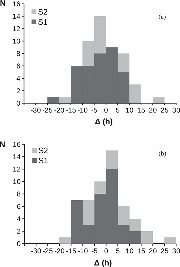
Figure 2. Distribution of the difference between ENLIL and DBM transit times, Δ = TTENLIL − TTDBM, for (a) Γ = 0.2 with w = 450 km s−1 and (b) Γ = 0.1 with w = 400 km s−1. Black and gray bars represent samples S1 and S2, respectively.
Download figure:
Standard image High-resolution imageIn Figure 3, the DBM-calculated transit times, TTDBM, are plotted as a function of ENLIL-calculated transit times, TTENLIL. The correlations are shown for Γ = 0.2 with w = 450 km s−1, Γ = 0.1 with w = 450 km s−1, and Γ = 0.1 with w = 400 km s−1. Note that the correlations for sample S2 (red crosses) show considerably larger scatter than the S1 correlations (blue circles), which is also evident from the linear-least-squares fit correlation coefficients, cc, summarized in Table 4. Furthermore, Table 4 shows that the slope of the correlations deviates from a = 1 and the y-axis intercept deviates from b = 0 (which would represent a perfect match), much more for S2 than for S1. Inspecting Table 4 and Figure 3, focusing on sample S1 in particular, one finds that the DBM model-input combination Γ = 0.1 with w = 400 km s−1 shows the closest match with the ENLIL results.
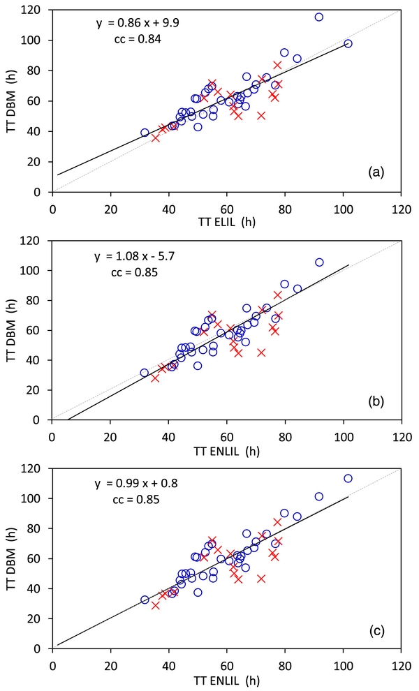
Figure 3. DBM-calculated vs. ENLIL-calculated transit times for (a) Γ = 0.2 with w = 450 km s−1, (b) Γ = 0.1 with w = 450 km s−1, and (c) Γ = 0.1 with w = 400 km s−1. Blue circles and red crosses represent samples S1 and S2, respectively. The linear-least-squares fit parameters shown in the insets are based on the combined sample S1+S2. The thin-dashed gray line represents a perfect match, y = x.
Download figure:
Standard image High-resolution imageTable 4. Overview of the Linear-least-squares Fit Parameters for the Correlation between ENLIL- and DBM-calculated Transit Times (TTDBM = a × TTENLIL + b) for Different Combinations of the DBM Model Parameters Γ and w
| Fit | S1 | S2 | S1+S2 | |
|---|---|---|---|---|
| Γ = 0.2 | a | 0.96 | 0.65 | 0.86 |
| w = 450 | b | +5.8 | +19.7 | +9.9 |
| cc | 0.89 | 0.73 | 0.84 | |
| Γ = 0.1 | a | 1.21 | 0.78 | 1.08 |
| w = 450 | b | −11.8 | +8.7 | −5.7 |
| cc | 0.91 | 0.73 | 0.85 | |
| Γ = 0.1 | a | 1.07 | 0.78 | 0.99 |
| w = 400 | b | −2.9 | +9.7 | +0.8 |
| cc | 0.91 | 0.73 | 0.85 | |
| Γ = 0.2 | a | 0.89 | 0.66 | 0.82 |
| w = 500 | b | +7.0 | +17.4 | +10.1 |
| cc | 0.91 | 0.72 | 0.85 |
Note. The correlation coefficient is denoted as cc; the y-axis intercept is expressed in hours.
Download table as: ASCIITypeset image
3.2. Comparison with the In Situ Measurements
In the following section, the forecasting performances of ENLIL and DBM are compared by checking the accuracy of the ICME arrival at Earth and STEREO. For that purpose, the in situ data from the L1-satellites Advance Composition Explorer (Stone et al. 1998) and WIND (Lin et al. 1995) were used, as well as the ICME data archive compiled by Richardson & Cane (2010), Lan Jian (UCLA/IGPP), Christian Möstl (University of Graz), and the "ISEST event list" (all lists can be found at http://solar.gmu.edu/heliophysics). The in situ shock arrivals at STEREO A and B were taken from the STEREO "level-3" data product where ICMEs and shocks are listed (available at http://www-ssc.igpp.ucla.edu/forms/stereo/stereo_level_3.html). If we found no corresponding event in that list, then we checked directly the "level-2" in situ measurements available at http://aten.igpp.ucla.edu/forms/stereo/level2_plasma_and_magnetic_field.html.
In Figure 4, we present the distribution of the observed-minus-calculated ICME transit times, O − C = TTobs − TTcalc for the sample S1*+S2*. The O − C values are based on the observed shock arrival for ENLIL and for the DBM input combination Γ = 0.2 with w = 450 km s−1. For both ENLIL and DBM, 66% of events arrived within ±18 hr relative to the "predicted" ICME arrival. The mean values are O − C = −0.3 ± 16.9 hr and −1.7 ± 18.3 hr, respectively, where averages of the absolute-value differences are very similar, equaling 14.1 hr and 14.8 hr.
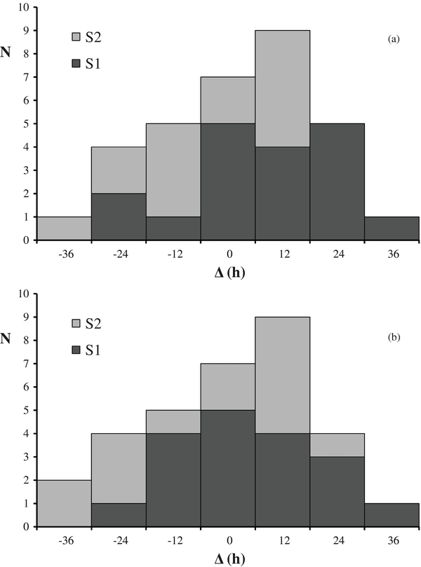
Figure 4. Distribution of the observed-minus-calculated shock transit times for the sample S1*+S2*: (a) ENLIL and (b) DBM for Γ = 0.2 with w = 450 km s−1. Black and gray bars represent samples S1* and S2*, respectively.
Download figure:
Standard image High-resolution imageIn Table 5, the average values, standard deviations, and root mean squares (RMSs) of the O − C values are summarized separately for samples S1*, S2*, and S1*+S2*. Inspecting the displayed data, one finds a significant difference between the S1* and S2* results. In the former sample, both ENLIL and DBM show positive O − C, i.e., the ICME arrived later than "predicted." The opposite is found for sample S2*, again indicating that the two samples are physically different. In this respect, it should be noted that S1* concerns events observed from 2010 April 3 to 2011 April 7, whereas S2* consists of events observed from 2012 March 13 to 2012 August 4. Though apparently not separated in time too much, these two periods belong to significantly different phases of the solar cycle. The former phase represents the very early rising phase of cycle 24, whereas the latter already belongs to a high-activity phase of the cycle. In other words, one can expect that, statistically, S1* and S2* ICMEs were propagating under different heliospheric conditions. The solar-cycle phase when S1* events occurred is usually characterized by a relatively flat heliospheric current sheet (see, e.g., Riley et al. 2002, and references therein) and the solar wind is "well-ordered" (see, e.g., McComas et al. 2008, and references therein). It should be noted that this is not necessarily true for individual events: for example, during CR2102 (2010 October 2 to 2010 October 29), the heliospheric current sheet was very complex (see, e.g., Robbrecht & Wang 2012), so some of the S1* ICMEs might have been propagating in a quite complex environment. On the other hand, in the case of S2* events, it could be expected that the heliospheric current sheet is strongly distorted and the solar wind becomes highly structured and variable. In addition, according to the LASCO observations, the CME activity was significantly lower in the S1* period than in the S2* period (e.g., the occurrence rate of halo CMEs was more than five times larger in the latter period), implying that the heliosphere was much more complex and dynamic in the latter case. Thus, one might speculate that from a statistical point of view, the propagation of S2* ICMEs was affected by a larger variety of parameters than in the case of S1* ICMEs, making the arrival prediction for S2* events less accurate. This is illustrated in Figure 5, where the observed TTs are displayed as a function of the CME mean speed, vCME, separately for S1* and S2* events. Note that the graph displays only the events measured in situ at Earth-L1, since the difference between heliocentric distances of the Earth-L1, STEREO-A, and STEREO-B is not negligible, i.e., the TTs for STEREO-A/STEREO-B would be systematically shifted to shorter/longer TTs, respectively. The graph shows that in the case of S1* events, there is a quite well-defined (anti)correlation between TT and VCME, as expected, whereas for S2* there is practically no relationship between these two parameters.
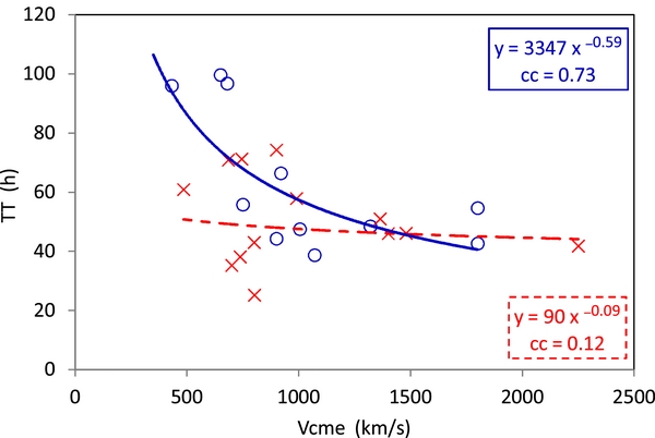
Figure 5. Observed ICME transit times vs. the CME speed, shown separately for sample S1* (blue circles) and S2* (red crosses). Only events measured at Earth-L1 are shown. The power-law fit parameters are shown in insets (S1*—top, S2*—bottom); the difference between the power-law exponents (i.e., the curve slopes), being −0.59 ± 0.18 for S1* and −0.09 ± 0.22 for S2*, has high statistical significance.
Download figure:
Standard image High-resolution imageTable 5. Summary of the Average Values ("aver"), Standard Deviations ("stdev"), and Root Mean Square ("RMS") of the Observed-minus-calculated Transit Times, O − C = TTobs − TTcalc, Expressed in Hours
| ENLIL | DBM | DBM | DBM | |
|---|---|---|---|---|
| Γ = 0.2 | Γ = 0.1 | Γ = 0.1 | ||
| w = 450 | w = 450 | w = 400 | ||
| aver S1* | +8.2 | +4.7 | +8.9 | +7.5 |
| stdev S1* | 16.7 | 15.7 | 15.1 | 15.1 |
| RMS S1* | 18.1 | 15.8 | 17.2 | 16.5 |
| aver S2* | −7.2 | −6.7 | −2.5 | −4.0 |
| stdev S2* | 14.2 | 19.2 | 20.8 | 20.9 |
| RMS S2* | 15.5 | 19.7 | 20.2 | 20.6 |
| aver S1*+S2* | −0.3 | −1.7 | +2.5 | +1.1 |
| stdev S1*+S2* | 16.9 | 18.3 | 19.0 | 19.1 |
| RMS S1*+S2* | 16.7 | 17.9 | 18.8 | 18.8 |
Download table as: ASCIITypeset image
The distribution of data points in Figure 5 is quite similar to analogous graphs presented by, e.g., Gopalswamy et al. (2001), Vršnak & Gopalswamy (2002), Schwenn et al. (2005), or Shanmugaraju & Vršnak (2014). Under the assumption of a constant ICME propagation speed (v = vCME), the data points should be grouped along the  curve. However, in all of these graphs, the distribution of data points significantly deviates from the
  curve. For example, the power-law fit shown in Figure 5 for S1* is characterized by an exponent of −0.59, which is significantly different from −1. Such behavior can be interpreted directly as the effect of drag, since slow CMEs are accelerated by the solar wind, whereas fast CMEs are decelerated. As a consequence, the TTs of slow/fast CMEs become shorter/longer, which decreases the slope of the TT(vCME) dependency (for a discussion, see, e.g., Shanmugaraju & Vršnak 2014, and references therein).
3.3. Solving the "Inverted Problem"
In Sections 3.1 and 3.2, various combinations of the DBM model-input parameters Γ and w have been applied, with the goal of finding a combination that provides the best overlap of the DBM and ENLIL outcomes and/or the DBM results and in situ measurements. In this section, we employ an alternative procedure (proposed by Vršnak et al. 2013) providing a combination of Γ and w for which the DBM-calculated TT equals a particular TT, in this case either ENLIL-calculated TT or the observed TT. Herein, we apply a simpler option of the procedure, seeking only the value of Γ for a fixed value of the solar-wind speed. It should be noted that a drawback of this "inverted-problem procedure" is that solutions do not exist for a certain fraction of events, due to specifications of the involved mathematical procedure (for details see Vršnak et al. 2013).
In Table 6, we present a summary of the average values ("aver") and standard deviations ("stdev") of the values of Γ calculated by the "inverted procedure" for different values of the background solar-wind speed w. The number of events for which solutions exists is denoted by n. The upper part of the table concerns the relationship between ENLIL and DBM, whereas the lower part relates in situ measurements and DBM.
Table 6. Summary of the Average Values ("aver") and Standard Deviations ("stdev") of the Values of Γ Calculated by the "Inverted Procedure" for Different Values of the Background Solar-wind Speed w
| w | ENLIL/DBM—S1 | ENLIL/DBM—S2 | ||||||
|---|---|---|---|---|---|---|---|---|
| (km s−1) | n | aver | stdev | n | aver | stdev | ||
| 400 | 16 | 0.20 | 0.07 | 11 | 0.37 | 0.23 | ||
| 450 | 17 | 0.25 | 0.14 | 8 | 0.46 | 0.42 | ||
| 500 | 22 | 0.61 | 0.60 | 8 | 0.49 | 0.44 | ||
| w | In Situ/DBM—S1 | In Situ/DBM—S2 | ||||||
| (km s−1) | n | aver | stdev | n | aver | stdev | ||
| 400 | 8 | 0.41 | 0.42 | 7 | 0.28 | 0.06 | ||
| 450 | 8 | 0.38 | 0.23 | 7 | 0.46 | 0.22 | ||
| 500 | 7 | 0.45 | 0.22 | 5 | 0.43 | 0.13 | ||
Notes. The number of events for which solutions exist is denoted by n. The upper part of the table concerns the relationship between ENLIL and DBM, whereas the lower part relates in situ measurements and DBM.
Download table as: ASCIITypeset image
In Figure 6, the results of the "inverted problem" procedure, showing the inferred values of the drag parameter Γ versus the applied background solar-wind speed, w, are presented graphically. Panel (a) considers a comparison of DBM and ENLIL, whereas panel (b) concerns a comparison of DBM and the observed TTs based on the in situ measurements. Inspecting the table and the graph, one finds somewhat higher values of Γ than expected from the results shown in previous sections. In this respect, we emphasize that the results are strongly dependent on the samples under study. Since the results are based on relatively small samples, the outcome of the inverted-problem procedure should be considered only as a rough estimate, still consistent (within the standard-deviation range) with the results presented in previous Sections 3.1 and 3.2.

Figure 6. Results of the "inverted problem" procedure, showing the inferred values of the drag parameter Γ vs. the applied background solar-wind speed, w, for adjusting (a) DBM with ENLIL and (b) DBM with in situ measurements.
Download figure:
Standard image High-resolution image
4. DISCUSSION AND CONCLUSIONS
The presented analysis showed that in a statistical sense, the Sun–Earth TTs calculated by the numerical model ENLIL are very similar to those provided by the analytical model DBM for drag-parameter values ranging between Γ = 0.1 and 0.2, combined with background solar-wind speeds ranging from w = 500 to 400 km s−1, respectively. The relative difference is most often less than 10% (see, e.g., Figure 3), and the average of the absolute-value differences is generally below 8 hr, depending on the combination of Γ and w applied in the DBM calculations. It should be noted that the difference becomes larger in periods of higher solar activity—the standard deviation of the differences between ENLIL- and DBM-calculated TTs (Table 3) ranges from ∼6 to ∼9 hr for sample S1 (low activity, simple background solar wind) and increases to ∼10–11 hr for sample S2 (high activity, complex background solar wind). This is a direct consequence of the ability of ENLIL to include a more realistic background solar-wind structure, which is not the case in the present form of DBM. Consequently, the difference between ENLIL and DBM becomes larger when the heliospheric situation becomes more complex.
We demonstrated that both models offer similar accuracy in predicting the ICME arrival at Earth (or STEREO), with the average of the observed-minus-calculated TT differences being around 14 hr. The corresponding standard deviation ranges from ∼14 to ∼19 hr depending on the sample and method. It is interesting to note (see Table 5) that DBM offers somewhat better predictions than ENLIL in the low-activity phase of the solar cycle (sample S1; standard deviations 15.1 and 16.7 hr, respectively; see Table 5), whereas the situation is reversed in the case of high activity (sample S2; standard deviations ∼20 and 14.2 hr, respectively) when the background solar wind becomes more complex. In this respect, we should emphasize that the error in the ICME arrival forecasting strongly depends on the sample. For example, Romano et al. (2013) analyzed a much larger sample of Earth-directed events than was employed herein and showed that a typical average absolute error in ENLIL real-time forecasts ranges between 7.5 and 12 hr, depending on the sample—all of the events together (71 arrivals) gave 9.5 hr. The "sampling effect" is also reflected in the differences between the results presented in Sections 3.1 and 3.2 relative to that presented in Section 3.3.
Finally, we should note that in the operation mode, as presented in this study, DBM and ENLIL use as input the CME parameters measured up to a distance ∼20 RS, which results in forecasting CME arrival and impact speed at 1 AU with lead times of about 2–4 days, depending on the speed of the CME. Instruments like the heliospheric imagers on board STEREO (or the future mission Solar Orbiter), covering radial distances much beyond 15 RS, may deliver more accurate kinematics extended to larger distances. This would certainly improve the accuracy of the arrival-time prediction, but with shorter lead times (e.g., Colaninno et al. 2013; Möstl et al. 2014). The optimal procedure would be to start with early predictions like those presented in this paper, and then successively adapt the results using new input data from instruments that cover larger distances. In this respect, it is advantageous to a certain degree to use DBM instead of ENLIL, as any user can easily feed the DBM public online tool with their own measurements to quickly recalculate the ICME-arrival prediction. Finally, let us emphasize that recently the WSA-ENLIL+Cone modeling was also made publicly available (http://ccmc.gsfc.nasa.gov/requests/SH/ENLIL-1cl/). Potentially, this offers the possibility to perform statistical analysis of the CME arrival predictions coming from different users applying different measurement techniques.
The research leading to these results has received funding from the European Commission's Seventh Framework Programme (FP7/2007-2013) under the grant agreement No. 263252 (COMESEP; www.comesep.eu) and No. 284461 (eHEROES; http://soteria-space.eu/eheroes/html/). M.T., A.V., and C.M. thank the Austrian Science Fund (FWF): V195-N16 and P26174-N27. A.T. greatly acknowledges Shota Rustaveli Foundation, Georgian National Science Foundation grant DI/14/6-310/12. This research was supported by a Marie Curie International Outgoing Fellowship within the 7th European Community Framework Programme.