


ABSTRACT
For Classical T Tauri Stars (CTTSs), the resonance doublets of N v, Si iv, and C iv, as well as the He ii 1640 Å line, trace hot gas flows and act as diagnostics of the accretion process. In this paper we assemble a large high-resolution, high-sensitivity data set of these lines in CTTSs and Weak T Tauri Stars (WTTSs). The sample comprises 35 stars: 1 Herbig Ae star, 28 CTTSs, and 6 WTTSs. We find that the C iv, Si iv, and N v lines in CTTSs all have similar shapes. We decompose the C iv and He ii lines into broad and narrow Gaussian components (BC and NC). The most common (50%) C iv line morphology in CTTSs is that of a low-velocity NC together with a redshifted BC. For CTTSs, a strong BC is the result of the accretion process. The contribution fraction of the NC to the C iv line flux in CTTSs increases with accretion rate, from ∼20% to up to ∼80%. The velocity centroids of the BCs and NCs are such that VBC ≳ 4 VNC, consistent with the predictions of the accretion shock model, in at most 12 out of 22 CTTSs. We do not find evidence of the post-shock becoming buried in the stellar photosphere due to the pressure of the accretion flow. The He ii CTTSs lines are generally symmetric and narrow, with FWHM and redshifts comparable to those of WTTSs. They are less redshifted than the CTTSs C iv lines, by ∼10 km s−1. The amount of flux in the BC of the He ii line is small compared to that of the C iv line, and we show that this is consistent with models of the pre-shock column emission. Overall, the observations are consistent with the presence of multiple accretion columns with different densities or with accretion models that predict a slow-moving, low-density region in the periphery of the accretion column. For HN Tau A and RW Aur A, most of the C iv line is blueshifted suggesting that the C iv emission is produced by shocks within outflow jets. In our sample, the Herbig Ae star DX Cha is the only object for which we find a P-Cygni profile in the C iv line, which argues for the presence of a hot (105 K) wind. For the overall sample, the Si iv and N v line luminosities are correlated with the C iv line luminosities, although the relationship between Si iv and C iv shows large scatter about a linear relationship and suggests that TW Hya, V4046 Sgr, AA Tau, DF Tau, GM Aur, and V1190 Sco are silicon-poor, while CV Cha, DX Cha, RU Lup, and RW Aur may be silicon-rich.
Export citation and abstract BibTeX RIS
1. INTRODUCTION
Classical T Tauri stars (CTTSs) are low-mass, young stellar objects surrounded by an accretion disk. They provide us with a laboratory in which to study the interaction between stars, magnetic fields, and accretion disks. In addition to optical and longer wavelength excesses, this interaction is responsible for a strong ultraviolet (UV) excess, Lyα emission, and soft X-ray excesses, all of which have a significant impact on the disk evolution, the rate of planet formation, and the circumstellar environment.
The observed long rotational periods, the large widths of the Balmer lines, and the presence of optical and UV excesses of CTTSs are naturally explained by the magnetospheric accretion paradigm (e.g., Uchida & Shibata 1984; Koenigl 1991; Shu et al. 1994). According to this paradigm, the gas disk is truncated some distance from the star (∼5 R*; Meyer et al. 1997) by the pressure of the stellar magnetosphere. Gas from the disk slides down the stellar gravitational potential along the magnetic field lines, reaching speeds comparable to the free-fall velocity (∼300 km s−1). These velocities are much larger than the local ∼20 km s−1 sound speed (but less than the Alfvén speed of ∼500 km s−1 implied by a 2 kG magnetic field; Johns-Krull 2007). The density of the accretion stream depends on the accretion rate and the filling factor but it is typically of the order of ∼1012 cm−3 (pre-shock; see Calvet & Gullbring 1998). The supersonic flow, confined by the magnetic field, produces a strong shock upon reaching the star, which converts most of the kinetic energy of the gas into thermal energy (e.g., Lamzin 1995).
The gas reaches temperatures of the order of a million degrees at the shock surface and cools radiatively until it merges with the stellar photosphere. Part of the cooling radiation will heat the stellar surface, resulting in a hot spot, observed spectroscopically as an excess continuum (the "veiling"). Cooling radiation emitted away from the star will illuminate gas before the shock surface, producing a radiative precursor of warm (T ∼ 104 K), ionized gas (Calvet & Gullbring 1998). In this paper we will use the term "accretion shock region" as shorthand for the region that includes the pre-shock, the shock surface, the post-shock column, and the heated photosphere.
Because the accretion column should be in pressure equilibrium with the stellar photosphere, Drake (2005) suggested that for typical accretion rates (∼10−8 M☉ yr−1) the post-shock region would be buried, in the sense that the shortest escape paths for post-shock photons would go through a significant column of photospheric gas. Sacco et al. (2010) have argued that the burying effects appear at accretion rates as small as a few times ∼10−10 M☉ yr−1 and that absorption of the X-rays by the stellar photosphere may explain the one to two orders of magnitude discrepancy between the accretion rates calculated from X-ray line emission and those calculated from optical veiling or near-UV excesses, and the lack of dense (ne ≳ 1011 cm−3) X-ray-emitting plasma in objects such as T Tau (Güdel et al. 2007).
Time-dependent models of the accretion column by Sacco et al. (2008) predict that emission from a single, homogeneous, magnetically dominated post-shock column should be quasi-periodic, on timescales of ∼400 s, because plasma instabilities can collapse the column. Such periodicity has not been observed (Drake et al. 2009; Günther et al. 2010), perhaps suggesting that accretion streams are inhomogeneous, or that there are multiple, uncorrelated accretion columns.
Observations during the last two decades have resulted in spectroscopic and photometric evidence for the presence of accretion hot spots or rings with filling factors of up to a few percent (see review by Bouvier et al. 2007). The surface topology of the magnetic field (e.g., Gregory et al. 2006; Mohanty & Shu 2008) and/or the misalignment between the rotational and magnetic axes result in a rotationally modulated surface flux (Johns & Basri 1995; Argiroffi et al. 2011, 2012), with a small filling factor (Calvet & Gullbring 1998; Valenti & Johns-Krull 2004). The spots appear and disappear over timescales of days (Rucinski et al. 2008) to years (Bouvier et al. 1993). Analysis of the possible magnetic field configurations indicates that although CTTSs have very complex surface magnetic fields, the portion of the field that carries gas from the inner disk to the star, is well ordered globally (Johns-Krull et al. 1999a; Adams & Gregory 2012).
In this paper we use the strong emission lines of ionized metals in order to probe the characteristics of the accretion shock region. In particular, we are interested in understanding the role that accretion has in shaping these lines, where the lines originate, and what the lines reveal about the geometry of the accretion process. Our long-term goal is to clarify the UV evolution of young stars and its impact on the surrounding accretion disk.
We analyze the resonance doublets of N v (λλ1238.82, 1242.80), Si iv (λλ1393.76, 1402.77), and C iv (λλ1548.19, 1550.77), as well as the He ii (λ1640.47) line. If they are produced by collisional excitation in a low-density medium, their presence suggests a high temperature (∼105 K, assuming collisional ionization equilibrium) or a photoionized environment. In solar-type main sequence stars, these "hot" lines are formed in the transition region, the narrow region between the chromosphere and the corona, and they are sometimes called transition-region lines.
The C iv resonance doublet lines are among the strongest lines in the UV spectra of CTTSs (Ardila et al. 2002). Using International Ultraviolet Explorer (IUE) data, Johns-Krull et al. (2000) showed that the surface flux in the C iv resonant lines can be as much as an order of magnitude larger than the largest flux observed in Weak T Tauri stars (WTTSs), main sequence dwarfs, or RS CVn stars. They also showed that the high surface flux in the C iv lines of CTTSs is uncorrelated with measures of stellar activity but it is strongly correlated with accretion rate, for accretion rates from 10−8 M☉ yr−1 to 10−5 M☉ yr−1. The strong correlations among accretion rate, C iv flux, and far-ultraviolet (FUV) luminosity have been confirmed by Ingleby et al. (2011) and Yang et al. (2012) using Advanced Camera for Surveys Solar Blind Channel (ACS/SBC) and Space Telescope Imaging Spectrograph (STIS) data. Those results further suggest a causal relationship between the accretion process and the hot line flux.
Previous surveys of the UV emission lines in low-resolution spectra of T Tauri stars include the analysis of IUE spectra (Valenti et al. 2000; Johns-Krull et al. 2000) and Goddard High Resolution Spectrograph (GHRS), ACS, and STIS spectra (Yang et al. 2012). Prior analysis of high resolution observations of the hot gas lines in T Tauri stars had been published for some objects (BP Tau, DF Tau, DG Tau, DR Tau, EG Cha, EP Cha, GM Aur, RU Lup, RW Aur A, RY Tau, T Tau, TW Hya, TWA 5, V4046 Sgr, and HBC 388; see Lamzin 2000a, 2000b; Errico et al. 2000, 2001; Ardila et al. 2002; Herczeg et al. 2002, 2005, 2006; Lamzin et al. 2004; Günther & Schmitt 2008; Ingleby et al. 2011). In addition, analysis of the C iv lines for the brown dwarf 2M1207 has been published by France et al. (2010). The observations show that the C iv lines in CTTSs have asymmetric shapes and wings that often extend to ±400 km s−1 from the line rest velocity. The emission lines are mostly centered or redshifted, although some stars occasionally present strong blueshifted emission (e.g., DG Tau, DR Tau, and RY Tau). Doublet ratios are not always 2:1 (e.g., DG Tau, DR Tau, RU Lup, and RW Aur A). Overall, the UV spectra of CTTSs also show large numbers of narrow H2 emission lines and CO bands in absorption and emission (France et al. 2011; Schindhelm et al. 2012), produced primarily by Lyα fluorescence. In most observations published so far, the Si iv line is strongly contaminated by H2 lines, and the N v 1243 Å line is absorbed by circumstellar or interstellar N i. High spectral resolution observations are crucial to fully exploit the diagnostic power of the UV observations as the H2 emission lines can be kinematically separated from the hot lines only when the resolution is high enough. In addition, we will show here that the hot gas lines have multiple kinematic components that can only be analyzed in high resolution spectra.
Both the correlation between accretion rate and C iv surface flux and the presence of redshifted hot gas line profiles in some stars, are consistent with formation in a high-latitude accretion flow. However, according to Lamzin (2003a, 2003b) C iv line formation in the accretion shock region should result in double-peaked line profiles, which are generally not observed. In this context Günther & Schmitt (2008) explored the shape of the hot gas lines (primarily O vi and C iv) in a sample of seven stars. They considered formation in the accretion shock, in an outflow, in the surface of the disk, in an equatorial boundary layer, and in the stellar transition region, and concluded that no single explanation or region can be responsible for all the observed line characteristics. In particular, they concluded that the shape of the redshifted lines was incompatible with models of magnetospheric accretion.
With the primary goal of providing a unified description of the hot gas lines and understanding their origin, we have obtained FUV and near-ultraviolet (NUV) spectra of a large sample of CTTSs and WTTSs, using the Cosmic Origins Spectrograph (COS) and the STIS. Most of the data for this paper comes from the Cycle 17 Hubble Space Telescope (HST) proposal "The Disks, Accretion, and Outflows (DAO) of T Tau stars" (PI: G. Herczeg; Prop. ID: HST-GO-11616). The DAO program is the largest and most sensitive high resolution spectroscopic survey of young stars in the UV ever undertaken and as such it provides a rich source of information for these objects. The program is described in more detail in G. Herczeg et al. (2013, in preparation). We have complemented the DAO data with GTO data from HST programs 11533 and 12036 (PI: J. Green; BP Tau, DF Tau, RU Lup, V4046 Sgr) as well as UV spectra from the literature and from the Mikulski Archive at STScI (Mikulski Archive for Space Telescopes, MAST).
As shown below, there is a wide diversity of profiles in all lines for the stars in our sample. The spectra are rich and a single paper cannot do justice to their variety nor to all the physical mechanisms that likely contribute to their formation. Here we take a broad view in an attempt to obtain general statements about accretion in CTTSs. Details about the sample and the data reduction are presented in Section 2. We then analyze the C iv, Si iv, He ii, and N v lines. The analysis of the C iv lines takes up most of the paper, as this is the strongest line in the set, and the least affected by absorptions or emissions by other species (Section 5). We examine the line shapes, the relationship with accretion rate, and correlations among quantities associated with the lines and other CTTSs parameters. We also obtain from the literature multi-epoch information on line variability (Section 5.4). The other lines play a supporting role in this analysis and are examined in Sections 6 and 7. Section 8 contains a summary of the observational conclusions and a discussion of their implications. The conclusions are in Section 9.
2. OBSERVATIONS
Tables 1–3 list the 35 stars we will be analyzing in this paper and the references for all the ancillary data we consider. Table 4 indicates the origin of the data (DAO or some other project), the data sets, and slit sizes used for the observations. Details about exposure times will appear in G. Herczeg et al. (2013, in preparation).
Table 1. Stars Analyzed in This Paper
| Name a | Alternate Name | Region | d | SpT b | Ref. SpT | Av | Ref. Av |
|---|---|---|---|---|---|---|---|
| (pc) | (mag) | ||||||
| Classical T Tauri Stars | |||||||
| AA Tau | HBC 63 | Taurus-Auriga | 140 | K7 | Donati et al. (2010) | 0.74 | Gullbring et al. (1998) |
| AK Sco | HBC 271 | Upper-Scorpius | 145 | F5+F5 | Andersen et al. (1989) | 0.5 | Alencar et al. (2003) |
| BP Tau | HBC 32 | Taurus-Auriga | 140 | K7 | Johns-Krull et al. (1999b) | 0.5 | Gullbring et al. (1998) |
| CV Cha | HBC 247 | Chamaeleon I | 160 | G8 | Guenther et al. (2007) | 1.5 | Furlan et al. (2009) |
| CY Tau | HBC 28 | Taurus-Auriga | 140 | M1 | Hartmann et al. (1998) | 0.32 | Gullbring et al. (1998) |
| DE Tau | HBC 33 | Taurus-Auriga | 140 | M0 | Furlan et al. (2009) | 0.62 | Gullbring et al. (1998) |
| DF Tau | HBC 36 | Taurus-Auriga | 140 | M2+? | Herczeg et al. (2006) | 0.6 | Herczeg et al. (2006) |
| DK Tau | HBC 45 | Taurus-Auriga | 140 | K7 | Furlan et al. (2009) | 1.42 | Gullbring et al. (1998) |
| DN Tau | HBC 65 | Taurus-Auriga | 140 | M0 | Furlan et al. (2009) | 0.25 | Gullbring et al. (1998) |
| DR Tau | HBC 74 | Taurus-Auriga | 140 | K7 | Petrov et al. (2011) | 1.2 | Gullbring et al. (2000) |
| DS Tau | HBC 75 | Taurus-Auriga | 140 | K5 | Muzerolle et al. (1998) | 0.34 | Gullbring et al. (1998) |
| DX Cha | HD 104237 |  Chamaeleontis Chamaeleontis | 114 | A7.5+K3 | Böhm et al. (2004) | 0.56 | Sartori et al. (2003) |
| EP Cha | RECX 11 | η Chamaeleontis | 97 | K4 | Mamajek et al. (1999) | 0 | Ingleby et al. (2013) |
| ET Cha | RECX 15 | η Chamaeleontis | 97 | M2 | Lawson et al. (2002) | 0 | Ingleby et al. (2013) |
| HN Tau A | HBC 60 | Taurus-Auriga | 140 | K5 | Furlan et al. (2009) | 0.65 | Gullbring et al. (1998) |
| MP Mus | PDS 66 | Isolated? | 100 | K1 | Torres et al. (2006) | 0.17 | Mamajek et al. (2002) |
| RU Lup | HBC 251 | Lupus I | 150 | K7 | Herczeg et al. (2005) | 0.1 | Herczeg et al. (2006) |
| RW Aur A | HBC 80 | Taurus-Auriga | 140 | K4+? | Johns-Krull et al. (1999b) | 1.2 | Valenti et al. (1993) |
| SU Aur | HBC 79 | Taurus-Auriga | 140 | G1 | Furlan et al. (2009) | 0.9 | Gullbring et al. (2000) |
| T Tau N | HBC 35 | Taurus-Auriga | 140 | K1 | Walter et al. (2003) | 0.3 | Walter et al. (2003) |
| V1190 Sco | HBC 617; Sz 102 | Upper Scorpius | 145 | K0 | Hughes et al. (1994) | 0.32 | Sartori et al. (2003) |
| V4046 Sgr | HBC 662 | β Pictoris | 72 | K5+K7 | Quast et al. (2000) | 0 | Curran et al. (2011) |
| Transition Disks | |||||||
| CS Cha | HBC 569 | Chamaeleon I | 160 | K6+? | Luhman (2004) | 0.3 | Furlan et al. (2009) |
| DM Tau | HBC 62 | Taurus-Auriga | 140 | M1.5 | Espaillat et al. (2010) | 0.6 | Ingleby et al. (2009) |
| GM Aur | HBC 77 | Taurus-Auriga | 140 | K5.5 | Espaillat et al. (2010) | 0.31 | Gullbring et al. (1998) |
| IP Tau | HBC 385 | Taurus-Auriga | 140 | M0 | Furlan et al. (2009) | 0.32 | Gullbring et al. (1998) |
| TW Hya | HBC 568 | TW Hydrae Association | 55 | K6 | Torres et al. (2006) | 0.0 | Herczeg et al. (2004) |
| UX Tau A | HBC 43 | Taurus-Auriga | 140 | K2 | Herbig (1977) | 0.7 | Furlan et al. (2009) |
| V1079 Tau | LkCa 15; HBC 419 | Taurus-Auriga | 140 | K3 | Espaillat et al. (2010) | 1.00 | White & Ghez (2001) |
| Weak T Tauri Stars | |||||||
| EG Cha | RECX 1 | η Chamaeleontis | 97 | K4+? | Mamajek et al. (1999) | 0 | Ingleby et al. (2013) |
| TWA 7 | 2MASS J1042-3340 | TW Hydrae Association | 55 | M2 | Torres et al. (2006) | 0 | Ingleby et al. (2009) |
| V1068 Tau | LkCa 4; HBC 370 | Taurus-Auriga | 140 | K7 | Herbig & Bell (1988) | 0.69 | Bertout (2007) |
| V396 Aur | LkCa 19; HD 282630 | Taurus-Auriga | 140 | K0 | Herbig & Bell (1988) | 0 | Walter et al. (1988) |
| V397 Aur | HBC 427 | Taurus-Auriga | 140 | K7+M2 | Steffen et al. (2001) | 0.0 | Kenyon & Hartmann (1995) |
| V410 Tau | HBC 29 | Taurus-Auriga | 140 | K2 (A) +M? (B) | Stelzer et al. (2003) | 0.03 | Bertout (2007) |
Notes. aIn this paper we refer to the stars with their variable star name, if it exists. The exception is TWA 7, which does not have a variable star name. bFor binary stars, the spectral type refers to the primary component, unless indicated.
Download table as: ASCIITypeset image
Table 2. Ancillary Data
| Name | Radial Velocity | Ref. Rad. Vel. | Inc. a | Ref. Inc. | Binarity b | Ref. Binarity |
|---|---|---|---|---|---|---|
| (km s−1) | (deg) | |||||
| Classical T Tauri Stars | ||||||
| AA Tau | 16.5 | Bouvier et al. (1999) | 70 ± 10 | Donati et al. (2010) | S | Najita et al. (2007) |
| AK Sco | −1.15 | Andersen et al. (1989) | 63 | Andersen et al. (1989) | 2 (SB) | Alencar et al. (2003) |
| BP Tau | 15.8 | Hartmann et al. (1986) | ∼45 | Donati et al. (2008) | S | Leinert et al. (1993) |
| CV Cha | 16.1 | Guenther et al. (2007) | 35 ± 10 | Hussain et al. (2009) | S | Melo (2003) |
| CY Tau | 19.1 | Hartmann et al. (1986) | 47 ± 8 | Simon et al. (2000) | S | Najita et al. (2007) |
| DE Tau | 14.9 | Hartmann et al. (1986) | 57 | Appenzeller et al. (2005) | S | Najita et al. (2007) |
| DF Tau | 11.0 | Edwards et al. (1987) | 50 | Appenzeller et al. (2005) | 2 (0 09) 09) | Ghez et al. (1993) |
| DK Tau | 15.3 | Hartmann et al. (1986) | 44 | Appenzeller et al. (2005) | 2 (2304) | Correia et al. (2006) |
| DN Tau | 16.1 | Hartmann et al. (1986) | 30 | Appenzeller et al. (2005) | S | Najita et al. (2007) |
| DR Tau | 27.6 | Alencar & Basri (2000) | 20 ± 4 | Petrov et al. (2011) | S | Leinert et al. (1993) |
| DS Tau | 16.3 | Hartmann et al. (1986) | ∼90 | Derived from | S | Najita et al. (2007) |
| Kundurthy et al. (2006) | ||||||
| Glebocki & Gnacinski (2005) | ||||||
| DX Cha | 13 | Kharchenko et al. (2007); | 18 | Grady et al. (2004) | 2 (SB) | Böhm et al. (2004) |
| EP Cha (RECX 11) | 18 | Assumed to be as EG Cha | N/A | ... | S | Brandeker et al. (2006) |
| ET Cha (RECX 15) | 15.9 | Barbier-Brossat & Figon (2000) | 40 | Woitke et al. (2011) | S | Woitke et al. (2011) |
| HN Tau A | 4.6 | Nguyen et al. (2012) | N/A | ... | 2 (A-B: 3109) | Correia et al. (2006) |
| MP Mus | 11.6 | Torres et al. (2006) | 32 | Curran et al. (2011) | S | Curran et al. (2011) |
| RU Lup | −0.9 | Melo (2003) | 24 | Herczeg et al. (2005) | S | Lamzin (1995) |
| RW Aur A | 14.0 | Hartmann et al. (1986) | 37 | Appenzeller et al. (2005) | M | Gahm et al. (1999); |
| (Aa-Ab: 001; AaAb-BC: 141) | Correia et al. (2006) | |||||
| SU Aur | 9.7 | Hartmann et al. (1986) | 52 ± 10 | Akeson et al. (2005) | S | Nguyen et al. (2012) |
| T Tau N | 19 | Hartmann et al. (1986) | 19 | Herbst et al. (1997) | 2 (07) | Dyck et al. (1982) |
| V1190 Sco | 5.0 | Graham & Heyer (1988) | <5 | Comerón & Fernández (2010) | N/A | ... |
| V4046 Sgr | −6.94 | Quast et al. (2000) | 35 | Quast et al. (2000) | 2 (SB) | Quast et al. (2000) |
| Transition Disks | ||||||
| CS Cha | 15.0 | Reipurth & Cernicharo (1995) | 60 | Espaillat et al. (2011) | 2 (SB)? c | Guenther et al. (2007) |
| DM Tau | 16.9 | Hartmann et al. (1986) | 45 ± 5 | Simon et al. (2000) | S | Najita et al. (2007) |
| GM Aur | 14.8 | Simon et al. (2000) | 54 ± 5 | Simon et al. (2000) | S | Najita et al. (2007) |
| IP Tau | 14.8 | Hartmann et al. (1987) | 30 | Derived from | S | Najita et al. (2007) |
| Glebocki & Gnacinski (2005) | ||||||
| Glebocki & Gnacinski (2005) | ||||||
| TW Hya | 13.5 | Sterzik et al. (1999); | 18 ± 10 | Herczeg et al. (2002) | S | Curran et al. (2011) |
| measured by Herczeg et al. (2002) | ||||||
| UX Tau A | 22.9 | Kharchenko et al. (2007); | 49 | Andrews et al. (2011) | S | Najita et al. (2007) |
| V1079 Tau (LkCa 15) | 17.0 | Hartmann et al. (1987) | 42 ± 5 | Simon et al. (2000) | S | Najita et al. (2007) |
| Weak T Tauri Stars | ||||||
| EG Cha (RECX 1) | 18 | Malaroda et al. (2000); | N/A | ... | M | Köhler & Petr-Gotzens (2002) |
| (AB 018; AB-C: 86) | ||||||
| TWA 7 | 10.6 | Kharchenko et al. (2007); | N/A | ... | S | Lowrance et al. (2005) |
| V1068 Tau (LkCa 4) | 16.9 | Hartmann et al. (1987) | N/A | ... | S | Najita et al. (2007) |
| V396 Aur (LkCa 19) | 14.3 | Hartmann et al. (1987) | N/A | ... | S | Najita et al. (2007) |
| V397 Aur | 15.0 | Walter et al. (1988) | N/A | ... | 2 (00328) | Steffen et al. (2001) |
| V410 Tau | 17.8 | Hartmann et al. (1986) | N/A | ... | M | Correia et al. (2006) |
| (AB: 007; AB-C: 0290) | ||||||
Notes. aInclination from face-on (=0°). When inclination is listed as "Derived from" we have derived it from the reported v*sin i, the period, and the stellar radius. bBinarity: S, single; M, multiple; SB, spectroscopic binary. The number in parenthesis indicates the separation of the components. cPossible spectroscopic long-period (>2482 days) binary. Unknown companion characteristics (Guenther et al. 2007).
Download table as: ASCIITypeset images: Typeset image Typeset image
Table 3. Ancillary Data
| Name |

| Ref. 
| Simult.  ?
a ?
a
|
|---|---|---|---|
| (10−8 M☉ yr−1) | Y/N | ||
| Classical T Tauri Stars | |||
| AA Tau | 1.3 | Ingleby et al. (2013) | Y |
| AK Sco | 1 | Assumed b | N |
| BP Tau | 2.9 | Ingleby et al. (2013) | N |
| CV Cha | 3.5 | Ingleby et al. (2013) | N |
| CY Tau | 0.75 | Gullbring et al. (1998) | N |
| DE Tau | 2.6 | Ingleby et al. (2013) | Y |
| DF Tau | 3.45 | Herczeg et al. (2006) - Average | N |
| DK Tau | 3.5 | Ingleby et al. (2013) | Y |
| DN Tau | 1.0 | Ingleby et al. (2013) | Y |
| DR Tau | 5.2 | Ingleby et al. (2013) | Y |
| DS Tau | 1.3 | Gullbring et al. (1998) | N |
| DX Cha | 3.55 | Garcia Lopez et al. (2006) | N |
| EP Cha (RECX 11) | 0.017 | Ingleby et al. (2013) | Y |
| ET Cha (RECX 15) | 0.042 | Ingleby et al. (2013) | Y |
| HN Tau A | 1.4 | Ingleby et al. (2013) | Y |
| MP Mus | 0.045 | Curran et al. (2011) | N |
| RU Lup | 1.8 | Herczeg et al. (2006) | N |
| RW Aur A | 2 | Ingleby et al. (2013) | Y |
| SU Aur | 0.55 | Calvet et al. (2004) | N |
| T Tau N | 4.45 | Calvet et al. (2004) | N |
| V1190 Sco | 0.79 | Güdel et al. (2010) | N |
| V4046 Sgr | 0.060 | Curran et al. (2011) | N |
| Transition Disks | |||
| CS Cha | 0.53 | Ingleby et al. (2013) | Y |
| DM Tau | 0.22 | Ingleby et al. (2013) | Y |
| GM Aur | 0.96 | Ingleby et al. (2013) | Y |
| IP Tau | 0.48 | Ingleby et al. (2013) | Y |
| TW Hya | 0.15 | Herczeg et al. (2004) - Average | N |
| UX Tau A | 1.1 | Espaillat et al. (2010) | N |
| V1079 Tau (LkCa 15) | 0.31 | Ingleby et al. (2013) | Y |
| Weak T Tauri Stars | |||
| EG Cha (RECX 1) | ... | ... | ... |
| TWA 7 | ... | ... | ... |
| V1068 Tau (LkCa 4) | ... | ... | ... |
| V396 Aur (LkCa 19) | ... | ... | ... |
| V397 Aur | ... | ... | ... |
| V410 Tau | ... | ... | ... |
Notes.
aSimultaneous (within ∼10 hr) near- and far-ultraviolet observations are available for some of the DAO targets (G. Herczeg et al. 2013, in preparation). The last column indicates whether simultaneous NUV observations were used to calculate the accretion rate, as described in Ingleby et al. (2013). bWe assume  = 1 × 10⁻⁸
M☉ yr−1 for AK Sco (Gómez de Castro 2009).
= 1 × 10⁻⁸
M☉ yr−1 for AK Sco (Gómez de Castro 2009).
Download table as: ASCIITypeset image
Table 4. Data Sources
| Name | FUV a | FUV Data Set b | FUV Slit c |
|---|---|---|---|
| Classical T Tauri Stars | |||
| AA Tau | DAO: COS G130M; G160M | LB6B070XX | PSA |
| AK Sco | DAO: STIS E140M | OB6B21040 | 02 × 02 |
| BP Tau | GTO 12036: COS G130M; G160M | LBGJ010XX | PSA |
| CV Cha | DAO: STIS E140M | OB6B180XX | 02 × 02 |
| CY Tau | GO 8206: STIS E140M | O5CF030XX | 02 × 02 |
| DE Tau | DAO: COS G130M; G160M | LB6B080XX | PSA |
| DF Tau | GTO 11533: COS G130M; G160M | LB3Q020XX | PSA |
| DK Tau | DAO: COS G130M; G160M | LB6B120XX | PSA |
| DN Tau | DAO: COS G130M; G160M | LB6B040XX | PSA |
| DR Tau | DAO: COS G130M; G160M | LB6B140XX | PSA |
| DS Tau | GO 8206: STIS E140M | O5CF010XX | 02 × 02 |
| DX Cha | DAO: STIS E140M | OB6B25050 | 02 × 02 |
| EP Cha | DAO: COS G130M; G160M | LB6B240XX | PSA |
| ET Cha | DAO: COS G130M; G160M | LB6B170XX | PSA |
| HN Tau A | DAO: COS G130M; G160M | LB6B090XX | PSA |
| MP Mus | DAO: STIS E140M | OB6B230XX | 02 × 02 |
| RU Lup | GTO 12036: COS G130M; G160M | LBGJ020XX | PSA |
| RW Aur | DAO: COS G130M; G160M | LB6B150XX | PSA |
| SU Aur | DAO: COS G130M; G160M | LB6B110XX | PSA |
| T Tau | GO 8157: STIS E140M | O5E3040XX | 02 × 006 |
| V1190 Sco | DAO: COS G130M; G160M | LB6B590XX | PSA |
| V4046 Sgr | GTO 11533: COS G130M; G160M | LB3Q010XX | PSA |
| Transition Disks | |||
| CS Cha | DAO: COS G130M; G160M | LB6B160XX | PSA |
| DM Tau | DAO: COS G130M; G160M | LB6B020XX | PSA |
| GM Aur | DAO: COS G130M; G160M | LB6B010XX | PSA |
| IP Tau | DAO: COS G130M; G160M | LB6B050XX | PSA |
| TW Hya | GO 11608: STIS E140M | OB3R070XX | 02 × 02 |
| UX Tau A | DAO: COS G130M; G160M | LB6B530XX | PSA |
| V1079 Tau | DAO: COS G130M; G160M | LB6B030XX | PSA |
| Weak T Tauri Stars | |||
| EG Cha | DAO: COS G130M; G160M | LB6B320XX | PSA |
| TWA 7 | DAO: COS G130M; G160M | LB6B300XX | PSA |
| V1068 Tau | DAO: COS G130M; G160M | LB6B270XX | PSA |
| V396 Aur | DAO: COS G130M; G160M | LB6B280XX | PSA |
| V397 Aur | DAO: COS G130M; G160M | LB6B260XX | PSA |
| V410 Tau | GO 8157: STIS E140M | O5E3080XX | 02 × 006 |
Notes.
aIn addition to the DAO data, we have made use of data from the following HST proposals: GO 8157: Molecular Hydrogen in the Circumstellar Environments of T Tauri Stars (PI: Walter); GO 8206: The Structure of the Accretion Flow on pre-main-sequence stars (PI: Calvet); GTO 11533: Accretion Flows and Winds of Pre-Main Sequence Stars (PI: Green); GO 11608: How Far Does H2 Go: Constraining FUV Variability in the Gaseous Inner Holes of Protoplanetary Disks (PI: Calvet); GTO 12036: Accretion Flows and Winds of Pre-Main Sequence Stars Part 2 (PI: Green). bThe data set columns indicate the suffix or the full name (if only one) of the HST data set used. cPSA: primary science aperture (for COS), 25 diameter. For the STIS data the slit size used is indicated.
Download table as: ASCIITypeset image
The data considered here encompass most of the published high resolution HST observations of the C iv doublet lines for CTTSs. Ardila et al. (2002) provide references to additional high-resolution C iv data for CTTSs obtained with the GHRS. We do not re-analyze those spectra here, but they provide additional context to our paper. Non-DAO STIS data were downloaded from the HST STIS Echelle Spectral Catalog of Stars (StarCAT; Ayres 2010). Non-DAO COS data were downloaded from the MAST and reduced as described below.
The sample of stars considered here includes objects with spectral types ranging from A7 (the Herbig Ae star DX Cha
18
) to M2, although most objects have mid-K spectral types. We assume stellar ages and distances to be ∼2 Myr and 140 pc, respectively, for Taurus-Aurigae (see Loinard et al. 2007 and references therein), ∼2 Myr and 150 pc for Lupus I (Comerón et al. 2009), ∼5 Myr and 145 pc for Upper-Scorpius (see Alencar et al. 2003 and references therein), ∼5 Myr and 114 pc for the Chamaeleontis cluster (see Lyo et al. 2008 and references therein), ∼5 Myr and 160 pc for Chamaeleon I (see Hussain et al. 2009 and references therein), ∼8 Myr and 97 pc for the η Chamaeleontis cluster (Mamajek et al. 1999), ∼10 Myr and 55 pc for the TW Hydrae association (Zuckerman & Song 2004), and ∼12 Myr and 72 pc for V4046Sgr in the β Pictoris moving group (Torres et al. 2006). The sample includes MP Mus (∼7 Myr and 100 pc; Kastner et al. 2010 and references therein), not known to be associated with any young region.
The sample includes stars with transition disks (TDs; Espaillat et al. 2011) CS Cha, DM Tau, GM Aur, IP Tau, TW Hya, UX Tau A, and V1079 Tau (LkCa 15). Here we take the term "transition disk" to mean a disk showing infrared evidence of a hole or a gap. As a group, TDs may have lower accretion rates than other CTTS disks (Espaillat et al. 2012). However, for the targets included here the difference between the accretion rates of TDs and those of the rest of the accreting stars is not significant. The sample also includes six Weak T Tauri Stars (WTTSs): EG Cha (RECX 1), V396 Aur (LkCa 19), V1068 Tau (LkCa 4), TWA 7, V397 Aur, and V410 Tau.
Of the 35 stars considered here, 12 are known to be part of binary systems. Dynamical interactions among the binary components may re-arrange the circumstellar disk or preclude its existence altogether. The presence of an unaccounted for companion may result in larger-than-expected accretion diagnostic lines. In addition, large instantaneous radial velocities may be observed in the targeted lines at certain points of the binary orbit.
AK Sco, DX Cha, and V4046 Sgr are spectroscopic binaries with circumbinary and/or circumstellar disks. CS Cha is a candidate long-period spectroscopic binary, although the characteristics of the companion are unknown (Guenther et al. 2007). The accretion rates listed in Table 3 are obtained from optical veiling and NUV excesses and represent total accretion for the overall system. At the end of this paper we will conclude that binarity may be affecting the line centroid determination only in AK Sco.
For non-spectroscopic binaries, the effect of the binarity may be relevant only if both companions are within the COS or STIS apertures. This is the case for DF Tau, RW Aur A, and the WTTSs EG Cha, V397 Aur, and V410 Tau. For DF Tau and RW Aur A, the primary component dominates the FUV emission (see Herczeg et al. 2006; Alencar et al. 2005).
Table 3 lists the accretion rate, obtained from literature sources. For some stars, the DAO data set contains simultaneous NUV and FUV observations, obtained during the same HST visit. Ingleby et al. (2013) describe those NUV observations in more detail and calculate accretion rates based on them. In turn, we use those accretion rate determinations here. The uncertainty in the accretion rate is dominated by systematic factors such as the adopted extinction correction and the color of the underlying photosphere. These may result in errors as large as a factor of 10 in the accretion rate. We do not list vsin i measurements for the sample but typical values for young stars are ∼10–20 km s−1 (Basri & Batalha 1990).
2.1. Data Reduction
The COS and STIS DAO data were all taken in time-tagged mode.
- 1.COS observations. The FUV (1150–1790 Å) spectra were recorded using multiple exposures with the G130M grating (1291, 1327 Å settings) and the G160M grating (1577, 1600, 1623 Å settings). These provide a velocity resolution of Δv ∼ 17 km s−1 (R ∼ 17,000) with seven pixels per resolution element (Osterman et al. 2011; Green et al. 2012).The maximum exposure time was accumulated in the region of the Si iv resonance lines and the exposures ranged from 3 ks (for most stars with two-orbit visits) to a maximum of 8 ks for a few stars with four-orbit visits. Use of multiple grating positions ensured full wavelength coverage and reduced the effects of fixed pattern noise.All observations were taken using the primary science aperture (PSA), which is a 25 diameter circular aperture. The acquisition observations used the ACQ/SEARCH algorithm followed by ACQ/IMAGE (Dixon & the COS/STIS Team 2011). The absolute wavelength scale accuracy is ∼15 km s−1 (1σ), where the error is dominated by pointing errors. We obtained one dimensional, co-added spectra using the COS calibration pipeline (CALCOS) with alignment and co-addition obtained using the IDL routines described by Danforth et al. (2010).
- 2.STIS observations. Those targets that are too bright to be observed by COS were observed using the STIS E140M echelle grating, which has a spectral resolution of Δv ∼ 7 km s−1 (R ∼ 45,000), over the region 1150–1700 Å. All the observations were obtained using the 02 × 02 "photometric" aperture, during two HST orbits.The STIS FUV spectra were calibrated and the echelle orders co-added to provide a single spectrum using the IDL software package developed for the StarCAT project (Ayres 2010). This reduction procedure provides a wavelength-scale accuracy of 1σ = 3 km s−1. Non-DAO STIS data were taken directly from StarCAT.
For a given pointing, errors in the positioning of the target within the aperture result in an offset in the wavelength scale. As indicated above, these are supposed to be 15 km s−1 for COS and 3 km s−1 for STIS, according to the instrument observing manuals (Dixon & the COS/STIS Team 2011; Ely & the COS/STIS Team 2011). In addition, the geometric correction necessary to account for the curvature of the COS FUV detector may make longer wavelength features appear redder than they really are. The offset depends on the exact position of the target on the detector. In most cases this intra-spectrum wavelength uncertainty is <10 km s−1, but in a few extreme cases it will introduce a ∼15 km s−1 shift from the reddest to the bluest wavelengths in a single COS grating mode (see Figure 4 from Linsky et al. 2012).
To determine how important the errors due to pointing and calibration are in the COS data, we focus on the H2 lines. We use the line measurements from K. France (2013, private communication; see also France et al. 2012) for P(2)(0–5) at 1398.95 Å, R(11)(2–8) at 1555.89 Å, R(6)(1–8) at 1556.87 Å, and P(5)(4–11) at 1613.72 Å. France et al. (2012) show that in the case of DK Tau, ET Cha (RECX 15), HN Tau, IP Tau, RU Lup, RW Aur, and V1079 Tau (LkCa 15), some H2 lines show a redshifted peak and a blueshifted low-level emission, which makes them asymmetric. Ignoring these stars, the four H2 lines are centered at the stellar rest velocity, with a standard deviations of 7.1, 6.5, 6.1, and 12.1 km s−1, respectively. The large scatter in the P(5)(4–11) line measurement is partly the result of low signal-to-noise in this region of the spectrum. Unlike the results reported by Linsky et al. (2012), we do not observe a systematic increase in the line center as a function of wavelength, neither star by star nor in the average of all stars for a given line. This is likely the result of the different acquisition procedure followed here. For the STIS data, the average standard deviation in all the H2 wavelengths is 4.4 km s−1.
This shows that the errors in the COS wavelength scale are smaller than the 15 km s−1 reported in the manuals and that no systematic shifts with wavelength are present. For the rest of the paper we will assume that the pointing errors in the COS data result in a velocity uncertainty of ±7 km s−1 (the average of the first three H2 lines considered) while the STIS errors are 5 km s−1. We do not correct the spectra for the H2 velocities, as it is not clear how to implement this correction in the case of stars with asymmetric H2 lines.
3. INTRODUCTION TO THE SHAPE OF THE LINES
Figures 14 and 15 in the Appendix show the lines that we are discussing in this paper. Each line is plotted in velocity space (km s−1) centered on the stellar photospheric rest frame. The ordinate gives flux density in units 10−14 erg s−1 cm−2 Å−1. In the case of doublets, the nominal wavelength of the strongest member of the line is set to zero velocity, and the positions of the strongest H2 lines are marked with dashed lines. Dotted lines mark the positions of other features in the spectra. The plotted spectra have been smoothed by a five-point median.
The C iv, Si iv, and N v lines are resonance doublets with slightly offset upper levels. For each doublet, both lines should have the same shape when emitted. This redundancy allow us to identify extra spectral features and to distinguish real features from noise. If the lines are emitted from an optically thin or effectively thin plasma, their flux ratio should be 2:1. If the lines are emitted from a medium that has a thermalization depth smaller than its optical depth (i.e., the medium is optically thick, but not effectively thin) the flux ratio will tend to 1.
For a plasma at rest in coronal ionization equilibrium, the peak ion abundance occurs at temperatures of log (T) = 5.3 (K) for N v, log (T) = 5.0 (K) for C iv, log (T) = 4.9 (K) for Si iv, and log (T) = 4.7 (K) for He ii (Mazzotta et al. 1998). In the context of the magnetospheric accretion paradigm, the velocities of the post-shock gas are high enough that the collisional timescales are longer than the dynamical timescale (Ardila 2007). This implies that the post-shock gas lines may trace lower temperature, higher density plasma than in the coronal ionization equilibrium case. The pre-shock plasma is radiatively ionized to temperatures of ∼104 K. If the pre- and post-shock regions both contribute to the emission, conclusions derived from the usual differential emission analyses are not valid (e.g., Brooks et al. 2001). In the case of non-accreting stars, the resonance N v, C iv, and Si iv lines are collisionally excited while the He ii line is populated by radiative recombination in the X-ray ionized plasma (Zirin 1975).
Figure 1 compares the hot gas lines of BP Tau and the WTTS V396 Aur. These stars provide examples of the main observational points we will make in this paper.
- 1.For N v and C iv the lines of the CTTSs have broad wings not present in the WTTSs. This is generally also the case for Si iv, although for BP Tau the lines are weak compared to H2.
- 2.The N v 1243 Å line of BP Tau (the redder member of the multiplet), and of CTTSs in general, looks truncated when compared to the 1239 Å line (the blue member), in the sense of not having a sharp emission component. This is the result of N i circumstellar absorption.
- 3.The Si iv lines in CTTSs are strongly affected by H2 lines and weakly affected by CO A-X absorption bands (France et al. 2011; Schindhelm et al. 2012) and O iv. At the wavelengths of the Si iv lines, the dominant emission seen in BP Tau and other CTTSs is primarily due to fluorescent H2 lines. The WTTS do not show H2 lines or CO bands within ±400 km s−1 of the gas lines we study here.
- 4.The C iv BP Tau lines have similar shapes to each other, to the 1239 N v line, and to the Si iv lines, when observed. Generally, the CTTS C iv lines are asymmetric to the red and slightly redshifted with respect to the WTTS line.
- 5.The He ii lines are similar (in shape, width, and velocity centroid) in WTTSs and CTTSs, and similar to the narrow component (NC) of C iv.
The general statements above belie the remarkable diversity of line profiles in this sample. Some of this diversity is showcased in Figure 2. For analysis and interpretation, we focus on the C iv doublet lines, as they are the brightest and "cleanest" of the set, with the others playing a supporting role. In order to test the predictions of the magnetospheric accretion model, in Section 5.3 we perform a Gaussian decomposition of the C iv profiles, and representative results are shown in Figure 2.

Figure 1. Comparison between the CTTS BP Tau (black line) and the WTTS V396 Aur (blue line) for the four emission lines we are analyzing. The vertical scale is arbitrary. The abscissas are velocities (km s−1) in the stellar rest frame. Solid lines: nominal line positions; dashed lines: nominal locations of the strongest H2 lines. N v, dotted lines: N i (1243.18 Å, +1055 km s−1; 1243.31 Å, +1085 km s−1). Si iv, dotted lines: CO A-X (5–0) bandhead (1392.5 Å, −271 km s−1), O iv (1401.17 Å, +1633 km s−1). He ii, dotted line: location of the secondary He ii line.
Download figure:
Standard image High-resolution image
Figure 2. The diversity of C iv CTTSs profiles. Dashed lines: narrow and broad Gaussian components; smooth solid lines: total model fit. The most common morphology is that of TW Hya, with a lower peak BC redshifted with respect to the NC. Stars like IP Tau have a BC blueshifted with respect to the NC. For V1190 Sco, both components have similar widths. For HN Tau the NC profile is blueshifted.
Download figure:
Standard image High-resolution imageTW Hya has a profile and decomposition similar to those of BP Tau: strong NC plus a redshifted, lower-peak broad component (BC). Of the stars for which a Gaussian decomposition is possible, ∼50% (12/22) show this kind of profile and ∼70% (21/29) of CTTSs in our sample have redshifted C iv peaks. HN Tau also has a NC plus a redshifted BC, but the former is blueshifted with respect to the stellar rest velocity by 80 km s−1. For IP Tau and V1190 Sco, the BC is blueshifted with respect to the NC. The magnetospheric accretion model may explain some of objects with morphologies analogous to TW Hya but blueshifted emission requires extensions to the model or the contributions of other emitting regions besides the accretion funnel (Günther & Schmitt 2008).
Figure 3 shows the C iv and He ii lines in all the WTTSs, scaled to the blue wings of the lines. For all except for V1068 Tau (Lk Ca 4) and V410 Tau, the C iv and He ii lines appear very similar to each other in shape, width, and shift. They are all fairly symmetric, with velocity maxima within ∼20 km s−1 of zero, and FWHM from 60 to 100 km s−1. V1068 Tau and V410 Tau have the largest FWHM in both C iv and He ii. The lines of these two stars appear either truncated or broadened with respect to the rest of the WTTSs. In the case of V410 Tau, vsin i = 73 km s−1 (Głe¸bocki & Gnaciński 2005), which means that rotational broadening is responsible for a significant fraction of the width. However, V1068 Tau has vsin i = 26 km s−1. For the rest of the WTTSs, vsin i ranges from 4 to 20 km s−1 (Głe¸bocki & Gnaciński 2005; Torres et al. 2006).

Figure 3. The WTTSs spectra in C iv and He ii. All the spectra have been scaled to have the same mean value in the wing between −150 and −50 km s−1. The solid vertical lines mark the rest-velocity positions of the C iv and He ii lines. Top: C iv. The dashed vertical line indicates the location at which the H2 line R(3)1–8 would be, if present. The large value of the TWA 7 line is an artifact of the scaling procedure, due to the line redshift (25.3 km s−1). Bottom: He ii. Except for V1068 Tau and V410 Tau, the WTTSs have similar characteristics (shape, shifts, and FWHM) in He ii and C iv. V1068 Tau and V410 Tau appear to be truncated or broadened in both lines.
Download figure:
Standard image High-resolution imageTo characterize the line shapes of He ii and C iv we have defined non-parametric and parametric shape measurements. The non-parametric measurements (Table 5) do not make strong assumptions about the line shapes and they provide a intuitive summary description of the line. These are the velocity at maximum flux, the FWHM, and the skewness, defined in Section 5.2. For C iv we have also measured the ratio of the 1548 Å to the 1550 Å line, by scaling the line wings to match each other. This provides a measure of the line optical depth. The parametric measurements (Tables 6 and 7) assume that each C iv and He ii line is a combination of two Gaussians.
Table 5. Non-parametric Line Measurements
| Name | C iv | He ii | |||||
|---|---|---|---|---|---|---|---|
| Ratio Blue/Red a | FWHM b | Vel. at max. flux c | Skewness d | FWHM e | Vel. at max. flux | Skewness f | |
| (km s−1) | (km s−1) | (km s−1) | (km s−1) | ||||
| Classical T Tauri Stars | |||||||
| AA Tau | 1.28 ± 0.1 | 207.4 | 32.2 ± 1 | 0.09 | 87.6 | 23.7 ± 1 | 0.01 |
| AK Sco | 1.89 ± 0.2 | 116.4 | −27.2 ± 2 | −0.06 | ... | ... | ... |
| BP Tau | 1.92 ± 0.1 | 82.9 | 14.1 ± 1 | 0.04 | 65.7 | −1.2 ± 1 | 0.01 |
| CV Cha | 2.15 ± 0.2 | 196.7 | −3.9 ± 6 | 0.01 | 53.7 | 5.7 ± 1 | 0.00 |
| CY Tau | 1.69 ± 0.3 | 45.5 | 19.6 ± 2 | 0.12 | 43.8 | −0.6 ± 2 | 0.02 |
| DE Tau | 1.38 ± 0.1 | 141.8 | 6.6 ± 2 | 0.00 | 81.6 | 9.0 ± 1 | 0.02 |
| DF Tau | 2.89 ± 0.1 | 96.3 | 17.5 ± 1 | −0.03 | 64.7 | 6.8 ± 1 | 0.01 |
| DK Tau | 1.79 ± 0.1 | 262.2 | −31.5 ± 1 | 0.05 | 83.6 | 8.3 ± 1 | 0.02 |
| DN Tau | 1.82 ± 0.1 | 74.9 | 19.0 ± 1 | 0.05 | 69.7 | −3.3 ± 1 | 0.01 |
| DR Tau | 1.52 ± 0.1 | 236.8 | 33.7 ± 1 | 0.07 | 66.7 | −12.4 ± 1 | 0.05 |
| DS Tau | 2.11 ± 0.1 | 61.5 | 15.5 ± 1 | 0.06 | 55.7 | 0.1 ± 2 | 0.01 |
| DX Cha | 1.24 ± 0.1 | 374.6 | 11.5 ± 1 | 0.07 | ... | ... | ... |
| EP Cha | 1.66 ± 0.1 | 153.8 | 21.2 ± 1 | 0.03 | 79.6 | −0.2 ± 1 | 0.01 |
| ET Cha | 1.24 ± 0.1 | 260.9 | −5.0 ± 1 | 0.03 | 80.6 | 6.1 ± 1 | −0.01 |
| HN Tau A | 1.67 ± 0.1 | 310.4 | −84.5 ± 1 | 0.05 | 226.9 | −82.9 ± 3 | 0.01 |
| MP Mus | 1.97 ± 0.2 | 267.6 | 9.8 ± 1 | −0.04 | 78.6 | −4.6 ± 2 | 0.02 |
| RU Lup | 1.26 ± 0.2 | 148.5 | 31.6 ± 2 | −0.05 | 90.5 | 19.6 ± 2 | 0.01 |
| RW Aur A | 1.45 ± 0.1 | 387.0 | −86.4 ± 1 | −0.021 | 131.7 | −99.2 ± 2 | 0.02 |
| SU Aur | 1.38 ± 0.1 | 335.8 | 44.3 ± 2 | −0.02 | 120.4 | 35.1 ± 1 | 0.00 |
| T Tau N | 1.71 ± 0.2 | 169.9 | −4.2 ± 1 | −0.07 | 79.5 | 4.9 ± 1 | −0.01 |
| V1190 Sco | 1.58 ± 0.2 | 251.5 | −2.7 ± 2 | −0.05 | 210.9 | 7.6 ± 2 | −0.05 |
| V4046 Sgr | 2.00 ± 0.1 | 301.0 | 55.3 ± 1 | 0.06 | 180.1 | 42.4 ± 1 | 0.00 |
| Transition Disks | |||||||
| CS Cha | 1.69 ± 0.1 | 235.8 | 32.0 ± 1 | 0.09 | 134.5 | 11.3 ± 1 | 0.01 |
| DM Tau | 1.72 ± 0.1 | 297.0 | 62.4 ± 1 | 0.06 | 75.6 | 7.5 ± 1 | 0.02 |
| GM Aur | 1.83 ± 0.1 | 270.2 | 26.0 ± 1 | −0.05 | 127.4 | −3.3 ± 1 | 0.02 |
| IP Tau | 1.27 ± 0.1 | 66.9 | 12.9 ± 1 | −0.06 | 87.6 | 8.0 ± 2 | 0.02 |
| TW Hya | 1.85 ± 0.1 | 247.5 | 26.4 ± 2 | 0.13 | 64.7 | 3.5 ± 1 | 0.04 |
| UX Tau A | 1.78 ± 0.1 | 290.8 | 1.3 ± 3 | −0.02 | 83.4 | −10.5 ± 1 | 0.03 |
| V1079 Tau | 1.89 ± 0.1 | 171.2 | 30.1 ± 1 | −0.01 | 68.7 | 14.9 ± 1 | 0.04 |
| Weak T Tauri Stars | |||||||
| EG Cha | 1.72 ± 0.1 | 88.3 | 9.5 ± 1 | 0.01 | 67.7 | −5.7 ± 1 | −0.01 |
| TWA 7 | 2.03 ± 0.1 | 59.4 | 12.3 ± 1 | 0.01 | 58.4 | −0.3 ± 1 | 0.00 |
| V1068 Tau | 1.74 ± 0.1 | 115.1 | 15.9 ± 1 | −0.02 | 96.5 | 11.6 ± 1 | −0.02 |
| V396 Aur | 2.14 ± 0.1 | 77.6 | 3.1 ± 1 | 0.00 | 74.6 | −12.6 ± 1 | 0.04 |
| V397 Aur | 1.91 ± 0.1 | 69.6 | −2.4 ± 1 | 0.01 | 77.6 | 18.0 ± 1 | −0.02 |
| V410 Tau | 2.15 ± 0.7 | 145.5 | 25.3 ± 7 | −0.01 | 136.3 | 13.7 ± 1 | −0.05 |
Notes. All velocities are calculated on the stellar rest frame. aThe ratio of the two C iv lines is calculated by matching the red wings of both lines between 0 and 150 km s−1. For RW Aur A, the scaling is calculated from 0 to 100 km s−1 only. bThis is the FWHM of the red C iv line. The error is ±5 km s−1. cVelocity at maximum flux for the C iv profile. Except for RW Aur A, this is the average of the two doublet lines. For RW Aur A it is only the velocity of the red line. dSkewness of the C iv profile, averaged over the two lines. For each line, skewness is defined as  , where
  is the flux-weighted mean velocity over an interval ΔV. For the blue and red lines, the intervals are ±250 km s−1 and ±150 km s−1 from the maximum, respectively. To calculate the average, we normalize the red C iv skewness to the blue one, by dividing by 250/150. To calculate the skewness, we have subtracted the continuum and interpolated over the H2 lines. Values of the skewness within ∼[−0.02, 0.02] indicate a symmetric line. eFWHM of the He ii line. The error is ±5 km s−1. fSkewness of the He ii profile. Measured over ±100 km s−1, but normalized to the C iv interval.
Download table as: ASCIITypeset image
Table 6. Gaussian Fits to the C iv Lines
| Blue Line | Red Line | |||||||||||||||
|---|---|---|---|---|---|---|---|---|---|---|---|---|---|---|---|---|
| Narrow Comp. | Broad Comp. | Narrow Comp. | Broad Comp. | |||||||||||||
| Name a | A0 | ΔA0 | V0 | ΔV0 | σ0 | Δσ0 | A1 | ΔA1 | V1 | ΔV1 | σ1 | Δσ1 | A2 | ΔA2 | A3 | ΔA3 |
| Flux | Flux | (km s−1) | (km s−1) | (km s−1) | (km s−1) | Flux | Flux | (km s−1) | (km s−1) | (km s−1) | (km s−1) | Flux | Flux | Flux | Flux | |
| Classical T Tauri Stars | ||||||||||||||||
| AA Tau (COS) | 2.81 | 0.1 | 23.65 | 0.3 | 17.50 | 0.2 | 2.70 | 0.1 | 82.86 | 0.4 | 120.94 | 0.5 | 2.78 | 0.1 | 1.37 | 0.1 |
| AK Sco (STIS) | 9.56 | 0.1 | −78.18 | 0.2 | 115.08 | 0.3 | 3.69 | 0.1 | −11.05 | 0.1 | 257.8 | 1 | 2.67 | 0.1 | 2.46 | 0.1 |
| BP Tau (COS) | 32.28 | 0.2 | 14.49 | 0.1 | 24.91 | 0.1 | 13.99 | 0.1 | 45.11 | 0.1 | 151.00 | 0.2 | 16.12 | 0.2 | 6.19 | 0.1 |
| BP Tau (GHRS) | 10.2 | 2 | 9.3 | 1 | 33.5 | 3 | 6.85 | 0.4 | −12.5 | 1 | 123.6 | 2 | 4.4 | 1 | 2.94 | 0.2 |
| CV Cha (STIS) | ... | ... | ... | ... | ... | ... | 4.43 | 0.2 | −4.77 | 0.1 | 140.04 | 0.3 | ... | ... | 2.16 | 0.1 |
| CY Tau (STIS) | 7.35 | 0.5 | 20.85 | 0.7 | 20.43 | 0.8 | 2.24 | 0.1 | 104.48 | 3.3 | 126.46 | 3.4 | 4.19 | 0.4 | 1.10 | 0.1 |
| DE Tau (COS) | 3.12 | 0.4 | 21.0 | 1 | 54.7 | 2 | 1.37 | 0.2 | 23.6 | 2 | 129.7 | 5 | 2.69 | 0.3 | 0.76 | 0.2 |
| DF Tau (COS) | 20.45 | 0.2 | 23.00 | 0.1 | 23.81 | 0.1 | 7.74 | 0.1 | −3.96 | 0.1 | 112.93 | 0.2 | 5.06 | 0.1 | 4.18 | 0.1 |
| DF Tau (GHRS) | 48.7 | 2 | 34.0 | 1 | 36.1 | 1 | 5.2 | 1 | −7.96 | 0.4 | 133.6 | 1 | 17.2 | 1 | 2.56 | 0.1 |
| DF Tau (STIS) | 49.0 | 2 | 26.54 | 0.4 | 19.65 | 0.3 | 7.43 | 0.3 | 26.0 | 1 | 104.3 | 2 | 14.5 | 1 | 3.52 | 0.2 |
| DK Tau (COS) | 0.45 | 0.1 | −20.7 | 8 | 25.3 | 8 | 0.93 | 0.1 | 36.4 | 3 | 142.5 | 6 | 0.23 | 0.1 | 0.49 | 0.1 |
| DN Tau (COS) | 10.86 | 0.1 | 21.33 | 0.1 | 28.87 | 0.2 | 2.92 | 0.1 | 63.76 | 0.4 | 120.79 | 0.5 | 6.22 | 0.1 | 1.26 | 0.1 |
| DR Tau (COS) | 1.55 | 0.3 | 80.7 | 4 | 80.2 | 4 | 1.02 | 0.2 | 98.4 | 6 | 197.2 | 9 | 1.38 | 0.2 | 0.35 | 0.1 |
| DR Tau (STIS) | ... | ... | ... | ... | ... | ... | 1.28 | 0.2 | 226.3 | 7 | 58.3 | 4 | ... | ... | 0.70 | 0.1 |
| DR Tau (GHRS 1995) | 1.7 | 1 | 112.2 | 7 | 50.8 | 4 | 1.54 | 0.4 | 17.1 | 2 | 76.4 | 5 | 2.5 | 1 | <0.2 | ... |
| DS Tau (STIS) | 38.9 | 1 | 27.61 | 0.2 | 23.34 | 0.3 | 5.71 | 0.2 | 57.3 | 1 | 147.4 | 2 | 23.5 | 1 | 2.32 | 0.1 |
| DX Cha b (STIS) | ... | ... | ... | ... | ... | ... | ... | ... | ... | ... | ... | ... | ... | ... | ... | ... |
| EP Cha (COS) | 3.84 | 0.1 | 28.94 | 0.3 | 30.25 | 0.3 | 5.20 | 0.1 | 40.17 | 0.2 | 136.23 | 0.3 | 2.31 | 0.1 | 2.74 | 0.1 |
| ET Cha (COS) | ... | ... | ... | ... | ... | ... | 1.58 | 0.1 | 9.76 | 0.2 | 99.80 | 0.4 | ... | ... | 0.98 | 0.1 |
| HN Tau A (COS) | 1.60 | 0.1 | −80.42 | 0.5 | 84.48 | 0.6 | 0.51 | 0.1 | 179.0 | 2 | 104.0 | 2 | 0.84 | 0.1 | 0.38 | 0.1 |
| MP Mus (STIS) | 18.49 | 0.1 | −4.47 | 0.1 | 74.92 | 0.1 | 22.63 | 0.1 | 6.06 | 0.1 | 153.34 | 0.1 | 12.96 | 0.1 | 10.16 | 0.1 |
| RU Lup (COS) | 12.09 | 0.1 | 36.63 | 0.1 | 43.36 | 0.1 | 6.77 | 0.1 | 0.03 | 0.1 | 192.95 | 0.1 | 11.07 | 0.1 | 3.85 | 0.1 |
| RU Lup (STIS) | 20 | 0.5 | 10.22 | 0.2 | 35.00 | 0.4 | 7.98 | 0.2 | −0.08 | 0 | 184.5 | 2 | 14.85 | 0.4 | 3.86 | 0.1 |
| RU Lup (GHRS) | ... | ... | ... | ... | ... | ... | 5.5 | 1 | −15 | 15 | 100.5 | 5 | ... | ... | 4.5 | 1 |
| RW Aur b (COS) | ... | ... | ... | ... | ... | ... | ... | ... | ... | ... | ... | ... | ... | ... | ... | ... |
| SU Aur (COS) | 1.00 | 0.3 | 85.2 | 7 | 113.2 | 9 | 1.88 | 0.3 | 17.0 | 1 | 160.3 | 5 | 1.03 | 0.3 | 1.02 | 0.3 |
| T Tau N (STIS) | 3.31 | 0.5 | −22.2 | 1 | 75.2 | 2 | 3.91 | 0.3 | −56.3 | 2 | 144.1 | 3 | 4.71 | 0.3 | <0.1 | ... |
| T Tau N (GHRS) | 6 | 0.2 | 0 | 0.2 | 79 | 0.5 | 3.5 | 0.1 | −52 | 1.2 | 152 | 0.7 | 5.3 | 0.2 | 0.25 | 0.1 |
| V1190 Sco (COS) | 3.55 | 0.1 | 9.44 | 0.1 | 83.97 | 0.1 | 1.50 | 0.1 | −103.54 | 0.1 | 104.13 | 0.1 | 2.24 | 0.1 | 1.00 | 0.1 |
| V4046 Sgr (COS) | 11.2 | 1 | 60.4 | 2 | 54.2 | 2 | 13.69 | 0.5 | 117.6 | 1 | 164.9 | 2 | 4.45 | 0.7 | 7.47 | 0.4 |
| Transition Disks | ||||||||||||||||
| CS Cha (COS) | 1.86 | 0.3 | 60 | 4 | 78.8 | 5 | 1.83 | 0.2 | 208.7 | 6 | 183.9 | 7 | 0.68 | 0.2 | 1.02 | 0.2 |
| DM Tau (COS) | ... | ... | ... | ... | ... | ... | 3.11 | 0.1 | 81.54 | 0.1 | 131.73 | 0.1 | ... | ... | 1.78 | 0.1 |
| GM Aur (COS) | 4.93 | 0.2 | 23.34 | 0.5 | 30.23 | 0.7 | 8.86 | 0.1 | 1.17 | 0.1 | 141.68 | 0.4 | 1.97 | 0.2 | 4.84 | 0.1 |
| IP Tau (COS) | 1.20 | 0.1 | 19.75 | 0.4 | 28.28 | 0.6 | 0.93 | 0.1 | −20.62 | 0.3 | 129.67 | 0.8 | 0.72 | 0.1 | 0.63 | 0.1 |
| TW Hya (STIS) | 122.93 | 2.2 | 27.74 | 0.3 | 35.32 | 0.3 | 133.68 | 0.9 | 116.58 | 0.3 | 142.43 | 0.3 | 55.02 | 1.5 | 73.64 | 0.6 |
| UX Tau A (COS) | ... | ... | ... | ... | ... | ... | 2.44 | 0.1 | 18.5 | 0.3 | 135.5 | 1 | ... | ... | 1.22 | 0.1 |
| V1079 Tau (COS) | 2.35 | 0.5 | 21.3 | 2 | 40.6 | 3 | 2.67 | 0.2 | 50.9 | 2 | 149.9 | 3 | 1.13 | 0.3 | 1.34 | 0.1 |
| Weak T Tauri Stars | ||||||||||||||||
| EG Cha (COS) | 2.91 | 0.1 | 4.16 | 0.1 | 33.41 | 0.1 | 1.03 | 0.1 | 1.42 | 0.2 | 104.19 | 0.1 | 1.75 | 0.1 | 0.53 | 0.1 |
| TWA 7 (COS) | 4.05 | 0.2 | 16.44 | 0.3 | 19.25 | 0.4 | 2.17 | 0.1 | 17.03 | 0.3 | 53.40 | 0.5 | 2.37 | 0.1 | 0.98 | 0.1 |
| V1068 Tau (COS) | 0.7 | 0.2 | −4.28 | 1 | 54.9 | 5 | 0.22 | 0.1 | 68.7 | 10 | 130.8 | 12 | 0.41 | 0.1 | 0.111 | 0.05 |
| V396 Aur (COS) | 2.06 | 0.7 | −4.03 | 1.5 | 29.10 | 4.2 | 0.44 | 0.1 | 7.57 | 0.4 | 101.82 | 1.2 | 1.07 | 0.5 | 0.24 | 0.1 |
| V397 Aur (COS) | 0.54 | 0.1 | −1.41 | 0.1 | 23.28 | 0.1 | 0.44 | 0.1 | −3.07 | 0.1 | 64.10 | 0.1 | 0.35 | 0.1 | 0.22 | 0.1 |
| V410 Tau (STIS) | 1.42 | 0.1 | −0.04 | 1.0 | 66.51 | 2.7 | ... | ... | ... | ... | ... | ... | 0.76 | 0.1 | ... | ... |
Notes. The flux has been fit in units of 10−14 erg s−1 cm−2. For each complex of two C iv lines we fit either two or four Gaussians. In the case of two Gaussians:  . In the case of four Gaussians:
  . aThe instrument used to obtain the data is indicated in parentheses. bFor DX Cha and RW Aur the red wing of the red line is different than the red wing of the blue line and neither a four nor an eight parameter fit is possible.
Download table as: ASCIITypeset images: Typeset image Typeset image
Table 7. He ii Gaussian Fits
| Name a | A0 | V0 | σ0 | A1 | V1 | σ1 |
|---|---|---|---|---|---|---|
| (10−14 erg s−1 cm−2) | (km s−1) | (km s−1) | (10−14 erg s−1 cm−2) | (km s−1) | (km s−1) | |
| Classical T Tauri Stars | ||||||
| AA Tau (COS) | 5.20 ± 0.1 | 25.54 ± 0.2 | 36.17 ± 0.3 | 0.47 ± 0.1 | 127.0 ± 3 | 219.2 ± 3 |
| AK Sco (STIS) | ... | ... | ... | ... | ... | ... |
| BP Tau (COS) | 38.75 ± 0.2 | 2.89 ± 0.1 | 29.76 ± 0.1 | 2.31 ± 0.1 | −2.13 ± 0.2 | 195.2 ± 1 |
| CV Cha (STIS) | 1.24 ± 0.2 | 10.5 ± 2.0 | 44.28 ± 3.8 | ... | ... | ... |
| CY Tau (STIS) | 6.72 ± 0.8 | 3.36 ± 0.6 | 21.37 ± 1.0 | 1.01 ± 0.4 | 15.0 ± 4 | 54.1 ± 8 |
| DE Tau (COS) | 1.24 ± 0.1 | 5.92 ± 0.1 | 25.28 ± 0.1 | 0.31 ± 0.1 | 21.18 ± 0.6 | 170.4 ± 2 |
| DF Tau (COS) | 12.62 ± 0.1 | 6.88 ± 0.1 | 24.71 ± 0.2 | 2.21 ± 0.1 | 36.14 ± 0.4 | 141.49 ± 0.8 |
| DK Tau (COS) | 2.92 ± 0.1 | 11.38 ± 0.4 | 32.43 ± 0.5 | 0.15 ± 0.1 | 44.20 ± 0.1 | 191.23 ± 0.4 |
| DN Tau (COS) | 13.18 ± 0.2 | −0.04 ± 0.1 | 31.38 ± 0.2 | 0.98 ± 0.1 | 72.5 ± 1 | 129.3 ± 2 |
| DR Tau (COS) | 1.22 ± 0.1 | −14.42 ± 0.5 | 28.66 ± 0.7 | 0.62 ± 0.1 | 104.9 ± 3 | 48.4 ± 2 |
| DS Tau (STIS) | 20.43 ± 0.7 | −1.53 ± 0.4 | 25.64 ± 0.4 | 3.83 ± 0.3 | 325.2 ± 3 | 33.6 ± 1 |
| DX Cha (STIS) | ... | ... | ... | ... | ... | ... |
| EP Cha (COS) | 6.92 ± 0.1 | −5.79 ± 0.2 | 28.79 ± 0.2 | 1.86 ± 0.1 | 25.74 ± 0.2 | 98.38 ± 0.4 |
| ET Cha (COS) | 1.51 ± 0.1 | −2.38 ± 0.1 | 20.47 ± 0.9 | 1.51 ± 0.1 | 1.15 ± 0.1 | 68.22 ± 0.7 |
| HN Tau A (COS) | 0.33 ± 0.1 | −89.34 ± 1.0 | 57.80 ± 0.8 | 0.23 ± 0.1 | 0.16 ± 0.1 | 204.1 ± 2 |
| MP Mus (STIS) | 17.80 ± 0.1 | −0.57 ± 0.1 | 25.15 ± 0.1 | 6.49 ± 0.1 | 6.83 ± 0.2 | 107.86 ± 0.4 |
| RU Lup (COS) | 7.27 ± 0.1 | 20.58 ± 0.1 | 35.78 ± 0.1 | ... | ... | ... |
| RW Aur (COS) | 0.78 ± 0.1 | −96.6 ± 3 | 27.2 ± 2 | 0.48 ± 0.1 | −48.5 ± 4 | 91.8 ± 5 |
| SU Aur (COS) | 2.26 ± 0.1 | 28.44 ± 0.1 | 43.37 ± 0.1 | 0.44 ± 0.1 | −0.15 ± 0.1 | 197.74 ± 0.9 |
| T Tau N (STIS) | 3.53 ± 0.3 | 0.14 ± 0.1 | 47.1 ± 2 | 0.79 ± 0.2 | 0.49 ± 0.1 | 146.5 ± 5 |
| V1190 Sco (COS) | 1.28 ± 0.1 | −23.37 ± 0.1 | 88.85 ± 0.1 | ... | ... | ... |
| V4046 Sgr (COS) | 19.24 ± 0.2 | 35.25 ± 0.2 | 66.85 ± 0.2 | 11.01 ± 0.2 | 58.01 ± 0.2 | 120.43 ± 0.4 |
| Transition Disks | ||||||
| CS Cha (COS) | 8.12 ± 0.1 | 17.53 ± 0.2 | 53.03 ± 0.3 | 1.03 ± 0.1 | 170.9 ± 3 | 191.6 ± 3 |
| DM Tau (COS) | 8.00 ± 0.1 | 7.74 ± 0.1 | 31.09 ± 0.2 | 1.65 ± 0.1 | 76.10 ± 0.9 | 132.79 ± 0.5 |
| GM Aur (COS) | 6.29 ± 0.1 | −5.24 ± 0.3 | 42.39 ± 0.5 | 1.78 ± 0.1 | 8.95 ± 0.8 | 209.0 ± 1 |
| IP Tau (COS) | 2.73 ± 0.1 | 11.46 ± 0.3 | 31.97 ± 0.3 | 0.15 ± 0.1 | 1.46 ± 0.1 | 163.50 ± 0.3 |
| TW Hya (STIS) | 292.00 ± 4.0 | −0.16 ± 0.1 | 21.99 ± 0.1 | 78.00 ± 2.1 | 49.18 ± 0.6 | 34.25 ± 0.5 |
| UX Tau A (COS) | 3.55 ± 0.2 | −0.25 ± 0.1 | 35.5 ± 1 | 0.65 ± 0.1 | 15.5 ± 2 | 150.4 ± 5 |
| V1079 Tau (COS) | 2.12 ± 0.1 | 16.00 ± 0.1 | 24.37 ± 0.1 | 0.67 ± 0.1 | 73.24 ± 0.4 | 44.27 ± 0.5 |
| Weak T Tauri Stars | ||||||
| EG Cha (W) (COS) | 6.31 ± 0.1 | −7.75 ± 0.1 | 27.70 ± 0.1 | 0.90 ± 0.1 | −4.98 ± 0.1 | 88.27 ± 0.1 |
| TWA 7 (COS) | 8.30 ± 0.3 | 0.15 ± 0.1 | 21.66 ± 0.3 | 1.85 ± 0.1 | 0.15 ± 0.1 | 55.1 ± 1 |
| V1068 Tau (W) (COS) | 0.94 ± 0.1 | 6.30 ± 0.1 | 48.15 ± 0.1 | ... | ... | ... |
| V396 Aur (W) (COS) | 2.56 ± 0.1 | −0.09 ± 0.1 | 33.88 ± 0.2 | 0.32 ± 0.1 | −1.75 ± 0.1 | 83.73 ± 0.2 |
| V397 Aur (W) (COS) | 1.37 ± 0.1 | 13.42 ± 0.1 | 33.80 ± 0.1 | ... | ... | ... |
| V410 Tau (W) (STIS) | 2.64 ± 0.2 | 11.3 ± 1 | 46.22 ± 2.0 | ... | ... | ... |
Notes. The He ii region of AK Sco is too noisy to allow the Gaussian fit. DX Cha does not show a single clear emission line in the spectral region. aWTTSs are indicated with a (W) after their name; the instrument used to obtain the data is indicated in parentheses.
Download table as: ASCIITypeset image
Table 8 lists the flux measurements that we will be considering in the following sections. The fluxes are obtained by direct integration of the spectra over the spectral range listed in the table, after subtracting the continuum and interpolating over known blending features (see Section 5).
Table 8. Hot Line Fluxes, Not Corrected for Extinction
| Name | N v (1238.8 Å) | N v (1242.8 Å) | Si iv (1393.8 Å) a | Si iv (1402.8 Å) a | C iv (1548.2 + 1550.8 Å) b | He ii (1640.5 Å) |
|---|---|---|---|---|---|---|
| (10−14 erg s−1 cm−2) | (10−14 erg s−1 cm−2) | (10−14 erg s−1 cm−2) | (10−14 erg s−1 cm−2) | (10−14 erg s−1 cm−2) | (10−14 erg s−1 cm−2) | |
| Classical T Tauri Stars | ||||||
| AA Tau | 0.221 ± 0.01 | 0.150 ± 0.01 | <0.3 | <0.3 | 8.66 ± 0.1 | 3.94 ± 0.1 |
| AK Sco | 2.43 ± 0.2 | 1.37 ± 0.2 | 10.2 ± 3 | 11.0 ± 3 | 37.6 ± 1 | <1 |
| BP Tau | 2.186 ± 0.02 | 0.984 ± 0.02 | 4.76 ± 0.3 | 3.34 ± 0.3 | 55.47 ± 0.1 | 23.20 ± 0.2 |
| CV Cha | 0.63 ± 0.1 | 0.09 ± 0.1 | 4.0 ± 1 | 3.6 ± 1 | 12.28 ± 0.1 | 1.78 ± 0.6 |
| CY Tau | 1.20 ± 0.1 | <0.3 | <4 | <4 | 9.10 ± 0.3 | 4.12 ± 0.9 |
| DE Tau | 0.475 ± 0.01 | 0.084 ± 0.01 | <0.5 | <0.5 | 8.68 ± 0.1 | 1.31 ± 0.2 |
| DF Tau | 1.080 ± 0.02 | 0.314 ± 0.02 | <0.9 | <0.8 | 25.69 ± 0.1 | 9.26 ± 0.2 |
| DK Tau | 0.145 ± 0.01 | 0.015 ± 0.01 | 0.68 ± 0.1 | 0.55 ± 0.1 | 3.503 ± 0.05 | 1.78 ± 0.2 |
| DN Tau | 0.901 ± 0.01 | 0.400 ± 0.01 | 1.20 ± 0.2 | 0.072 ± 0.01 | 13.07 ± 0.1 | 7.51 ± 0.2 |
| DR Tau | 0.287 ± 0.01 | <0.03 | 1.46 ± 0.3 | 1.27 ± 0.3 | 8.71 ± 0.1 | 1.31 ± 0.3 |
| DS Tau | 0.84 ± 0.1 | 0.23 ± 0.1 | 3.0 ± 1 | 2.7 ± 1 | 35.93 ± 0.5 | 11.8 ± 1 |
| DX Cha | 35.92 ± 0.6 | 5.90 ± 0.6 | 218 ± 10 | 169 ± 10 | 147.1 ± 2 | N/A |
| EP Cha | 0.983 ± 0.01 | 0.399 ± 0.01 | 0.98 ± 0.1 | 0.62 ± 0.1 | 16.57 ± 0.7 | 5.62 ± 0.1 |
| ET Cha | 0.411 ± 0.01 | 0.254 ± 0.01 | <0.5 | <0.5 | 3.619 ± 0.03 | 2.10 ± 0.1 |
| HN Tau A | 0.2837 ± 0.007 | 0.1335 ± 0.007 | 1.90 ± 0.2 | 1.67 ± 0.2 | 4.132 ± 0.04 | 0.97 ± 0.1 |
| MP Mus | 5.68 ± 0.1 | 2.49 ± 0.1 | 8.6 ± 1 | 4.9 ± 1 | 94.3 ± 1 | 17.30 ± 1.0 |
| RU Lup | 2.574 ± 0.05 | 0.308 ± 0.05 | 25.9 ± 1 | 18.8 ± 1 | 44.8 ± 1 | 5.79 ± 0.5 |
| RW Aur A | 0.812 ± 0.02 | 0.038 ± 0.01 | 4.68 ± 0.4 | 4.66 ± 0.4 | 6.00 ± 0.1 c | 1.85 ± 0.3 |
| SU Aur | 0.463 ± 0.01 | 0.202 ± 0.01 | 1.26 ± 0.2 | 1.54 ± 0.2 | 9.53 ± 0.1 | 2.59 ± 0.2 |
| T Tau N | 1.14 ± 0.1 | 0.55 ± 0.1 | 3.1 ± 1 | 2.8 ± 1 | 16.15 ± 0.1 | 5.89 ± 1.0 |
| V1190 Sco | 0.700 ± 0.01 | 0.354 ± 0.01 | <0.4 | <0.4 | 9.65 ± 0.1 | 1.63 ± 0.1 |
| V4046 Sgr | 29.66 ± 0.1 | 10.43 ± 0.1 | <1 | <1 | 57.10 ± 0.1 | 38.05 ± 0.2 |
| Transition Disks | ||||||
| CS Cha | 2.491 ± 0.03 | 0.848 ± 0.02 | <0.8 | <0.7 | 9.93 ± 0.1 | 9.01 ± 0.2 |
| DM Tau | 0.853 ± 0.02 | 0.281 ± 0.02 | <0.4 | <0.4 | 8.57 ± 0.1 | 7.11 ± 0.1 |
| GM Aur | 2.383 ± 0.03 | 0.662 ± 0.03 | <1 | <1 | 28.23 ± 0.2 | 8.50 ± 0.2 |
| IP Tau | 0.1211 ± 0.006 | 0.0491 ± 0.006 | 0.34 ± 0.1 | 0.31 ± 0.1 | 3.560 ± 0.04 | 1.64 ± 0.1 |
| TW Hya | 38.30 ± 0.6 | 17.13 ± 0.4 | 8.8 ± 3 | 7.6 ± 3 | 473.4 ± 2 | 228.9 ± 4 |
| UX Tau A | 0.949 ± 0.03 | 0.391 ± 0.01 | 1.08 ± 0.2 | 0.73 ± 0.2 | 6.9 ± 0.1 | 2.80 ± 0.3 |
| V1079 Tau | 0.485 ± 0.01 | 0.136 ± 0.01 | 1.32 ± 0.2 | 1.11 ± 0.2 | 9.80 ± 0.1 | 1.78 ± 0.1 |
| Weak T Tauri Stars | ||||||
| EG Cha | 0.948 ± 0.01 | 0.460 ± 0.01 | 1.76 ± 0.1 | 1.08 ± 0.1 | 4.111 ± 0.05 | 3.50 ± 0.1 |
| TWA 7 | 0.759 ± 0.02 | 0.399 ± 0.01 | 1.03 ± 0.2 | 0.68 ± 0.2 | 3.925 ± 0.04 | 4.03 ± 0.1 |
| V1068 Tau | 0.0813 ± 0.004 | 0.0428 ± 0.004 | 0.116 ± 0.03 | 0.0064 ± 0.001 | 1.412 ± 0.03 | 0.69 ± 0.1 |
| V396 Aur | 0.2335 ± 0.008 | 0.1118 ± 0.008 | 0.52 ± 0.1 | 0.298 ± 0.07 | 2.357 ± 0.04 | 1.47 ± 0.1 |
| V397 Aur | 0.0895 ± 0.004 | 0.0455 ± 0.004 | 0.142 ± 0.04 | 0.082 ± 0.02 | 0.855 ± 0.02 | 0.75 ± 0.1 |
| V410 Tau | 0.30 ± 0.1 | <0.3 | <3 | <3 | 2.37 ± 0.2 | 2.51 ± 0.8 |
Notes. aMeasured fluxes not corrected for extinction. The fluxes were obtained by integrating between −400 km s−1 and 400 km s−1, except for EG Cha. For this star, the Si iv flux was obtained by integrating from −800 to 600 km s−1. bMeasured fluxes not corrected for extinction. The flux has been measured from −400 to 900 km s−1, interpolating over the R(3)1–8 H2 line. cThe C iv line flux for RW Aur A was obtained by creating a synthetic blue line, as a copy of the red C iv line but scaled by 1.4.
Download table as: ASCIITypeset image
4. THE RELATIONSHIP BETWEEN ACCRETION RATE AND C iv LUMINOSITY
As mentioned in the introduction, Johns-Krull et al. (2000) showed that the accretion rate is correlated with excess C iv luminosity. The excess C iv luminosity is obtained by subtracting the stellar atmosphere contribution to the observed line. They estimated the stellar contribution to be 6 × 10⁻⁵ L☉ for a 2 R☉ object. They also showed that the correlation of C iv excess luminosity with accretion rate is very sensitive to extinction estimates. More recently, Yang et al. (2012) obtain a linear correlation between the C iv luminosity (from STIS and ACS/SBC low-resolution spectra) and the accretion luminosity (from literature values) for 91 CTTSs. Here we show that our data are consistent with a correlation between accretion rate C iv luminosity and explore the role that the lack of simultaneous observations or different extinction estimates play in this relationship.
Figure 4 compares accretion rates (references given in Table 1) with the C iv line luminosities. Blue diamonds correspond to objects with simultaneous determinations of  and
and  when available (Ingleby et al. 2013) and green diamonds correspond to
  determinations for the rest of the objects. Note that the accretion rate estimates from Ingleby et al. (2013) are derived using the extinction values from Furlan et al. (2009, 2011).

Figure 4. Accretion rate vs. C iv luminosity. The blue diamonds correspond to stars with simultaneous determinations of accretion rate and line luminosity. The red diamonds are objects with non-simultaneous determinations of accretion rate. The solid line is the correlation obtained by using all of the diamonds. Black triangles use the extinctions from Furlan et al. (2009, 2011) to calculate  . Errors in
  /L☉ are ∼5%–10%. The dashed line is Equation (2) from Johns-Krull et al. (2000), assuming R* = 2 R☉ for all stars. The lowest luminosity blue diamond corresponds to ET Cha (RECX 15) which has R* = 0.9 R☉ (Siess et al. 2000).
Download figure:
Standard image High-resolution imageUsing only the simultaneous values (blue diamonds), we obtain a Pearson product-moment correlation coefficient r = 0.73 (p-value = 0.3%
19
) while with all values we obtain r = 0.61 (p-value ⩽ 0.05%). The difference between using all of the data or only the simultaneous data is not significant for the purposes of the correlation. Including all data, we obtain  , where
  is given in M☉ yr−1 and the errors indicate 1σ values obtained by the bootstrap method. The correlation is plotted in Figure 4.
As argued by Johns-Krull et al. (2000), the observed relationship between  and accretion rate is very sensitive to extinction estimates. This is shown in Figure 4, for which the C iv luminosities indicated by the black triangles were calculated using the extinction estimates from Furlan et al. (2009, 2011), for all the targets we have in common with that work. For
  and
and  the correlation is weakened when using the Furlan et al. (2009, 2011) extinction values: the value of the Pearson's r is 0.44, with p-value = 5%.
The extinction values we adopt in this paper come from a variety of sources, but a significant fraction come from Gullbring et al. (1998, 2000). They argue that the colors of the WTTSs underlying the CTTSs are anomalous for their spectral types, which biases the near-IR extinction estimates. They obtain the extinctions reported here by deriving models of the UV excess in CTTSs. For other stars, we have adopted extinction estimates based on spectroscopic observations of the accretion veiling, when possible. The extinction values from Furlan et al. (2009, 2011) are obtained by de-reddening the observed near-infrared colors until they match the colors for the target's spectral type. They are significantly larger than the values we adopt in this paper, resulting in larger estimates of the C iv luminosity. Differences in the extinction estimates can have a substantial impact in the adopted flux, as a 10% increase in the value of AV results in a 30% increase in the de-reddened C iv line flux.
Figure 4 also shows the relationship between accretion rate and C iv luminosity derived by Johns-Krull et al. (2000, their Equation (2)) assuming that all stars have a radius of 2 R☉. They obtained their relationship based on the accretion rates and extinctions from Hartigan et al. (1995). Both of those quantities are higher, on average, than the ones we adopt here, and so their correlation predicts larger accretion rates. Note that the relationship from Johns-Krull et al. (2000) is not defined for stars with excess C iv surface fluxes smaller than 106 erg s−1 cm−2.
Overall, there is enough evidence to confirm that for most CTTSs the C iv line luminosity is powered primarily by accretion, and we will adopt this hypothesis here. However, the exact relationship between accretion rate and C iv luminosity remains uncertain. This is not surprising considering the complexity of the processes that contribute to the line flux, as we show in this work. The dominant uncertainty is the exact value of the extinction, which depends on the assumed stellar colors and on the shape of the extinction law in the UV (Johns-Krull et al. 2000; Calvet et al. 2004).
We do not detect a monotonic decrease in the CTTSs C iv luminosity as a function of age, for the range of ages considered here (2–10 Myr). We do not observe a significant difference in the C iv luminosities of the TDs as compared with the rest of the sample, consistent with the results from Ingleby et al. (2011) who found no correlations between FUV luminosities and tracers of dust evolution in the disk.
5. THE C iv LINE SHAPE
The C iv lines of CTTSs are generally redshifted, broad (with emission within ∼400 km s−1 of the stellar rest velocity), and asymmetric to the red (positive skewness). We will show that none of these characteristics is correlated with the line luminosity or with accretion rate.
5.1. Comparing the Two C iv Lines
If optically thin, both C iv lines form should have the same shape. Differences between the components can help us discover the presence of extra sources of absorption or emission. To exploit this redundancy, in Figure 16 we plot both members of the C iv doublet, with the 1550 Å line scaled to match the 1548 Å one. The scaling is done by matching the line peaks or the line wings from ∼0 to ∼150 km s−1. We expect this scaling factor to be 2 for optically thin or effectively thin emission. However, as we discuss in Section 5.2.4, the opacity characteristics of the broad and narrow line components are different, and the overall scaling factor may not be the best predictor of opacity.
Figure 16 shows that the line wings tend to follow each other closely, at least until about +200 to +300 km s−1, when the 1548 Å line start to bump into the 1550 Å one. The 1548 Å line is usually contaminated by the H2 line R(3)1–8 (1547.3 Å), at −167 km s−1 with respect to its rest velocity (e.g., DK Tau). Figure 16 also reveals examples of extra emission at ∼−100 km s−1 which do not appear in the 1550 Å line (AK Sco, DE Tau, DK Tau, DR Tau, HN Tau A, RU Lup, and UX Tau A). We tentatively identify emission from Fe ii (1547.807, −73.6 km s−1 from the rest velocity of the 1548 C iv line), C ii (1547.465; −139.8 km s−1), and Si i (1547.452 Å, −142.3 km s−1; 1547.731 Å, −88.3 km s−1), for these stars, as responsible for the emission to the blue of the C iv 1548 Å line.
To measure the C iv line flux listed in Table 8 we subtracted the continuum and interpolated over the H2 R(3)1–8 line and the Si i, C ii, Fe ii-complex, when present. The resulting spectrum is then integrated from −400 km s−1 to 900 km s−1 of the 1548 C iv line. We also detect the CO A-X (0–0) absorption band at 1544.4 Å (−730 km s−1 from the 1548 Å line; see France et al. 2011; McJunkin et al. 2013) in a significant fraction of the sample. The wing of the CO absorption may extend to the blue edge of the 1548 C iv line. However, its impact in the overall C iv flux is negligible.
Note that the red wings of each C iv line for DX Cha, RW Aur A, DF Tau, and RU Lup do not follow each other, and AK Sco and CS Cha have extra emission features near the 1550 Å.
For DX Cha we will argue in Section 8 that the peculiar shape of the C iv lines can be explained by the existence of a hot wind.
The strange appearance of C iv lines of RW Aur A is due to a bipolar outflow (see Figure 5). France et al. (2012) show that the H2 lines from RW Aur A are redshifted by ∼100 km s−1 in at least two progressions ([v', J'] = [1, 4] and [1, 7]), as they originate in the receding part of the outflow. In the observations we present here, the C iv doublet lines are blueshifted by ∼−100 km s−1, as can be seen from the position of the 1550 C iv line. This points to an origin in the approaching part of the outflow. The net result of these two outflows is that the blueshifted 1548 C iv line is buried under the redshifted H2 emission. RW Aur A is the only unequivocal example of this coincidence in the current data set. For HN Tau A the H2 R(3) 1–8 line is also redshifted, although the redshift (+30 km s−1) is within the 2σ of the error introduced by the pointing uncertainty (see also France et al. 2012). Therefore, HN Tau A may be another object for which we are observing two sides of the outflow, although the velocities of the blueshifted and redshifted sides do not match as well as in RW Aur.
For DF Tau, the apparent red wing in the 1550 Å line is an artifact of the line scaling, because for this star the ratio between the two C iv lines is almost 3, indicating either extra absorption or emission in one of the components. Unlike the case in RW Aur A, redshifted H2 emission is not responsible for the extra emission, as the R(3) 1–8 line is observed at −167 km s−1. Other observations show that the ratio between the two lines remains high among different epochs (Section 5.4). The origin of this extra emission in the 1548 Å line or absorption in the 1550 Å one remains unexplained in this work.
For RU Lup, the extra "bump" 200 km s−1 to the red of the 1548 Å C iv line is also present in other epoch observations of the system and remains unexplained in this work. AK Sco and CS Cha also present anomalous profiles, but of a different kind. AK Sco shows a broad emission −250 km s−1 from the 1550 Å line, not present in the 1548 Å line. CS Cha also shows and extra emission in the 1550 Å line at ∼−100 km s−1 and ∼+200 km s−1.
5.2. Non-parametric Description
5.2.1. The Velocity of the Peak Emission as a Function of Luminosity and Accretion Rate
The velocity of peak emission for each line is defined as the mean velocity of the top 5% of the flux between −100 and +100 km s−1 (for the 1548 C iv line) or between +400 and +600 km s−1 (for the 1550 Å line). This is calculated from spectra that have been smoothed by a five-point median. The velocity of peak listed in Table 5 is the average of both lines.
The C iv line is centered or redshifted for 21 out of 29 CTTSs, uncorrelated with line luminosity or accretion rate (Figure 6, top). The most significant exceptions are: DK Tau which shows two emission peaks, one blueshifted and the other redshifted, present in both lines; HN Tau A, for which both C iv lines have an emission peak at ∼−80 km s−1 from their rest velocity; 20 RW Aur A, for which the peak of the 1550 Å line is at −86 km s−1. In the case of AK Sco there is extra emission in the 1548 Å line that may be due to Si i but there is also extra emission ∼−250 km s−1 from the 1550 Å line. It is unclear therefore, whether the C iv lines are centered or blueshifted, although both the Si iv and the N v lines (which follow the C iv lines) are well centered. Those four stars are among the higher accretors in the sample and have jets seen in the high-velocity components of forbidden lines (Hartigan et al. 1995). Four other CTTSs have slightly blueshifted peaks, but with velocities > − 4 km s−1.
The average velocity at maximum flux for the C iv CTTSs lines is  km s−1 (Table 9). In this paper the uncertainties refer to uncertainties in the calculated mean values, not including the four stars with strong blueshifts (DK Tau, HN Tau A, and RW Aur A for which outflowing material is contributing to the profile, nor AK Sco, for which the two C iv lines are different from each other). We have argued that the velocity uncertainties for this COS data set are ∼7 km s−1. A one-sample Kolmogorov–Smirnov (KS) test confirms that the probability of the observed distribution being normal centered at zero, with 1σ = 7 km s−1 is negligibly small. The conclusion is the same if we take 1σ = 15 km s−1, the nominal wavelength error for COS. In other words, the overall redshift of the CTTSs C iv lines is significant.
Table 9. Average Line Kinematic Parameters
| Parameter | WTTSs C iv | CTTSs C iv | WTTSs He ii | CTTSs He ii |
|---|---|---|---|---|
| (km s−1) | (km s−1) | (km s−1) | (km s−1) | |
| Non-parametric Averages (Section 5.2) | ||||
| VMax | 10.6 ± 4 | 18.3 ± 4 a | 4.1 ± 5 | 7.1 ± 3 a |
| FWHM | 92 ± 10 | 210 ± 18 | 85 ± 11 | 96 ± 9 |
| Skewness | −0.005 ± 0.01 | 0.018 ± 0.01 | −0.007 ± 0.01 | 0.0126 ± 0.004 |
| Parametric Averages (Section 5.3) | ||||
| VNC | 1.6 ± 2 | 26.6 ± 6 a | 3.9 ± 3 | 6.0 ± 3 a |
| VBC | 17.2 ± 5 | 39 ± 10 a | −2.2 ± 1 | 53 ± 20 a |
| FWHMNC | 91 ± 20 | 118 ± 10 | 83 ± 10 | 85 ± 10 |
| FWHMBC | 223 ± 40 | 334 ± 30 | 178 ± 20 | 335 ± 30 |
| Velocity Differences b | ||||
 − VMax − VMax
| 7.7 ± 6 a | 0 | 14.2 ± 6 a | 11.0 ± 4 |
 − VMax − VMax
| 0 | −7.7 ± 6 a | 6.5 ± 6 | 3.4 ± 6 a |
 − VNC − VNC
| 24.8 ± 7 a | 0 | 22.7 ± 7 a | 19.7 ± 6 |
 − VNC − VNC
| 0 | −24.8 ± 7 a | −2.2 ± 5 | −4.4 ± 3 a |
 − VBC − VBC
| 21 ± 20 a | 0 | 39.2 ± 10 a | −4 ± 10 a |
 − VNC − VNC
| 38 ± 10 a | 26 ± 17 | 39 ± 10 a | 42 ± 10 |
 − VNC − VNC
| 4.4 ± 3 a | −19.7 ± 6 | 2.1 ± 4 a | 0 |
 − VNC − VNC
| 2.2 ± 5 | −39.2 ± 10 a | 0 | −2.1 ± 4 a |
Notes. All calculations include the H2 velocity correction (Section 2.1). aDoes not include HN Tau, RW Aur, AK Sco. bVelocity differences measured in the same spectrum (for example  −
−  ) are not subject to errors due to pointing.
Download table as: ASCIITypeset image
The WTTSs are also redshifted, with  km s−1. A two-sided KS test comparing the CTTSs and WTTSs VMax distribution gives p-value = 0.6, which indicates that they are consistent with the null hypothesis. In other words, although the mean velocity of the WTTSs is ∼2σ less that the mean CTTS velocity, the observations are consistent with the two quantities having the same distribution. Linsky et al. (2012) have shown that for rotation periods such as those observed in T Tauri stars, the Si iv and C iv lines in low-mass dwarfs present redshifts of ∼7 km s−1, the result of gas flows produced by magnetic heating. Given the scatter in their sample, our redshifts in WTTSs are consistent with theirs.
5.2.2. The Line Width as a Function of Luminosity and Accretion Rate
Overall, most of the CTTSs C iv lines show detectable emission within ±400 km s−1 of the nominal velocity. The FWHM is measured using the 1550 Å line of the smoothed C iv spectrum. The smoothing is the same used to measure the velocity of maximum flux.
Figure 6 (second row) shows that, as a group, the C iv WTTSs lines are narrower ( km s−1) than the CTTSs ones (
 km s−1). The p-value of the KS test comparing the two samples is 0.02, implying that the difference is significant.
The WTTS also have a smaller FWHM range (from 60 to 145 km s−1) than the CTTSs (from 45 to 387 km s−1). Note that the FWHM of the WTTSs is comparable to that of the CTTSs in some stars, the result of the strong NC dominating the CTTS lines (see, for example, the C iv lines for DS Tau in Figure 14(b)). The FWHM clearly fails to capture most relevant information regarding the line as it does not take into account the multi-component nature of the lines.
The observed FWHM is uncorrelated with line luminosity or accretion rate. The plots in Figure 6 (second row) suggest that the FWHM scatter increases with accretion rate, but this apparent increase is not statistically significant.
5.2.3. The Skewness as a Function of Luminosity and Accretion Rate
In Figure 6 (third row) we plot skewness versus C iv luminosity. The skewness compares the velocity of the peak to the mean velocity of the profile. It is defined as  , where VMax is the velocity at maximum flux and
  is the flux-weighted mean velocity over an interval ΔV centered on the maximum velocity. To calculate the skewness of the C iv line, we subtracted the continuum and interpolated over the H2 lines present in the C iv intervals. For the 1548 and 1550 Å lines,
  is measured within ±250 km s−1 and ±150 km s−1 from the maximum, respectively. To make the values comparable, we normalize to ΔV = 250 km s−1 in each line. The 1548 Å and 1550 Å values are then averaged.
Qualitatively, values of skewness within ∼ ± 0.02 indicate a symmetric line. Positive values indicate a line extending to the red. The absolute value of the skewness serves as a quantitative measure of asymmetry. 70% (20/29) CTTS have skewness greater or equal to zero, with 52% (15/29) having positive (>0.02) skewness.
All the WTTS have skewness values consistent with symmetric lines. A KS test comparing both populations shows that the difference in asymmetry is significant (p-value = 0.002).
As with FWHM, the skewness is uncorrelated with line luminosity or accretion rate.
5.2.4. The Line Scaling as a Function of Luminosity and Accretion Rate
The fourth row panels of Figure 6 compare the ratios of the 1548 Å to the 1550 Å C iv lines as a function of  (left) and
  (right). These are not flux ratios, but the scaling factors used to match both line profiles in Figure 16. As mentioned before (Section 5.1), the scaling factors between the C iv lines are indicative of the line's optical depth compared to the thermalization depth (Table 8).
All WTTSs and over half of the CTTSs (19/29—66%; 6/7—86% of TD, 12/22—55% of the non-TD) have ratios >1.65, consistent within the errors with thin or effectively thin emission. The difference in line opacity between stars with TDs and those without is not significant. For the rest of CTTSs, 10/29 (34%) have ratios which are consistent with small absorption mean free paths.
We do not observe a correlation between this measure of opacity and either line luminosity or accretion rate. The apparent increase in scatter at high accretion rates is not significant, according to a two-sided KS test (p-value = 0.6). Furthermore, objects with C iv ratios <1.7 are found for all luminosities and accretion rates.
As indicated in Section 5.1, DF Tau presents a particular case for which the scaling factor is significantly >2, an impossible value unless there is extra emission in the 1548 Å line or extra absorption in the 1550 Å one.
5.2.5. The Role of the Inclination in the Measured Luminosity and Accretion Rate
Geometric explanations are often invoked in the literature to explain the shapes of these emission lines. For example, Lamzin et al. (2004) suggest that the observed accretion in TW Hya occurs at low stellar latitudes, and that the lack of separate line components coming from the pre- and post-shock in other stars may be due to equatorial layer accretion.
Figure 6 (bottom) shows the relationship between inclination and line luminosity or accretion rate. We do not observe particularly larger or smaller fluxes at high or low inclinations. According to the KS test, the distributions of  and
and  are the same between objects with i > 45° and those with i ⩽ 45°. Also, the distribution of inclinations for objects with high
  or high
  is statistically the same that for objects with low
  or low
  . In particular, the apparently empty region in the panel at high inclinations and low accretion rates is not significant and does not provide evidence that the disk or the accretion flow are obscuring the accretion diagnostics. Furthermore, we do not find any significant correlations between the line ratio, VMax, FWHM, or skewness, and inclination.
If the C iv lines originate in a localized accretion stream one would expect to detect more stars at low inclinations than at high inclinations: for face-on systems the accretion stream will always be visible, while for systems almost edge-on this is not the case, if the region below the disk is blocked from view. For a random distribution of accretion spot positions in the stellar hemisphere, we expect to see an accretion spot in 58% of stars with 0° < i < 45° and in 42% of stars with 45° < i < 90° (ignoring disk flaring). In our sample, we have 37% of targets with inclinations larger than 45°, and the standard deviation of this count is 10%. Therefore, the observed difference in the number of stars with high and low inclinations is not significant. Over a hundred CTTSs with known inclinations are needed before we can distinguish 42% from 58% at the 3σ level. The current inclination data set is not complete enough to reveal geometric information about the C iv lines.
On the other hand, one could assume that the C iv UV lines are not emitted from a particular place but covers the whole star. For a given star, the C iv luminosity should then decrease linearly, by a factor of two, as the inclination increases from 0° to 90°. We do not observe this effect either, indicating, at least, that the observed scatter is dominated by intrinsic differences in the objects and not by geometry.
5.2.6. Conclusions from the Non-parametric Analysis
In conclusion, WTTS and CTTS C iv lines have comparable velocities at maximum flux, but the CTTS lines are generally broader and more asymmetric. In the case of CTTSs, neither the velocity of maximum flux, the FWHM, the skewness of the line, nor the ratio between the two C iv lines are correlated with C iv luminosity or accretion rate. The right column panels from Figure 6 do show increased scatter in these quantities as the accretion rate increases, suggesting that objects with large accretion rates have more diverse line shapes. However, the differences in the distributions (of the velocity, FWHM, skewness) with high and low accretion rates are not significant. More observations of stars with accretion rates ⩽4 × 10⁻⁹ M☉ yr−1 are needed. Among the three pairs of shape quantities (VMax versus FWHM, FWHM versus Skewness, VMax versus Skewness) there are no significant correlations.
The scaling of the 1548 Å line to the 1550 Å one should be 2 if the lines are emitted from a thin or effectively thin medium. This is the case in all the WTTSs and in about 70% of CTTSs. This measure of the opacity is not correlated with accretion rate or line luminosity. However, in Section 5.3.1 we show that the NC of the line is correlated with accretion rate.
There are no correlations between line shape parameters and inclination or between inclination and accretion rate or line luminosity, but we conclude that the data are not complete enough for inclination to be a strong descriptor in the sample.
5.3. C iv Gaussian Decomposition
Different regions of the T Tauri system may be contributing to the C iv lines. In the context of the magnetospheric accretion paradigm, the pre- and post-shock regions should be the dominant sources of the observed line emission. Shocks in an outflow, hot winds, and the stellar atmosphere may also contribute to the emission. To examine the line kinematics of the different regions we decompose each C iv line in one or two Gaussian functions. We are not asserting that the mechanism giving origin to the lines produces Gaussian shapes, although turbulent flows will do so (Günther & Schmitt 2008). Representative decompositions are shown in Figure 2.
The primary goal of the Gaussian decomposition is to obtain widths and centroids for the main line components. According to the magnetospheric accretion model, post-shock emission lines should have small velocity centroid distribution about the stellar rest frame velocity, and if no turbulence is present, the lines should be narrow. Pre-shock emission lines, which likely originate in a larger volume upstream from the accretion flow (Calvet & Gullbring 1998), should have larger velocity centroid distribution in the stellar rest frame and broader lines.
Table 6 presents the results of fitting one or two Gaussians to each of the C iv lines, after subtracting the continuum and interpolating over the H2 line R(3)1–8, and the Si i, C ii, Fe ii-complex, when present. For each target, we assume that the C iv lines are always separated by 500.96 km s−1, and that they have the same shape. This results in a four-parameter fit when fitting one Gaussian to each line: height for the 1548 Å line; height for the 1550 Å line; width σs; centroid velocity for the 1548 Å line. When fitting two Gaussians to each line, we have an eight-parameter fit: For the 1548 Å line, the heights of the broad (ABC) and narrow (ANC) components; analogous parameters for the 1550 Å line; σ for the BC; σ for the NC; centroid velocities for the broad (VBC) and narrow (VNC) components of the 1548 Å line.
Table 6 also indicates whether the data were taken with COS (possible systematic wavelength error assumed to be 7 km s−1) or STIS (possible systematic wavelength error of 3 km s−1). We also list the parameters derived for the multi-epoch observations of BP Tau, DF Tau, DR Tau, RU Lup, and T Tau N that we will consider in Section 5.4.
Wood et al. (1997) analyzed the C iv lines of 12 stars with spectral types F5 to M0. They found that the observed line profiles could be better fit with both a narrow and a broad Gaussian component, than with a single Gaussian component. For the type of stars included in their sample (dwarfs, giants, spectroscopic binaries, and the Sun), the C iv line is a transition-region line, as it is in the WTTSs. Because of this, we fitted both NCs and BCs to all the WTTSs, except V410 Tau. For V410 Tau, each C iv line can be well fitted with only one NC, although this may just be the result of the low S/N in the spectrum.
When comparing the two C iv lines in Section 5.1, we mentioned that AK Sco, CS Cha, DX Cha, DF Tau, RU Lup, and RW Aur A were objects for which the line doublet members had different shapes and/or extra unidentified emission in one of the doublet members. We do not perform the Gaussian decomposition for RW Aur A or DX Cha. For AK Sco, we list the parameters derived from the Gaussian fits (Table 6), but we do not use these results when exploring correlations. For the rest, we interpolate the profiles over the apparent the extra emission.
For four objects (CY Tau, DM Tau, ET Cha, and UX Tau A) we decompose the C iv lines in only one broad Gaussian component. For the rest of the CTTSs, the decomposition requires both a narrow and a broad Gaussian components, and Figure 7 shows the distributions of velocity centroids and FWHM. Average velocity and FWHM values are given in Table 9. Typical FWHMs of CTTS NCs range from 50 to 240 km s−1, with an average of 130 km s−1, while BCs widths range from 140 to a 470 km s−1, with an average of 350 km s−1. The velocity centroids range from −100 km s−1 to 200 km s−1. The BC velocity is larger than the NC velocity in 70% of the CTTS sample, and the distribution of BC velocities tend to be more positive ( km s−1) than that of the NC velocities (
 km s−1), giving some of the profiles the characteristic "skewed to the red" shape.
5.3.1. The Optical Depth as a Function of Accretion
Figure 8 (top) shows the ratio of the height of the NC in the 1548 Å line to the NC in the 1550 Å C iv line as a function of accretion rate, as well as the ratio of the heights of the BCs. Most observations are grouped around 2 although there is a lot of scatter, particularly at high accretion rates. The plot reveals that the NC of DF Tau is anomalous (>2), while the BC has an optically thin ratio. Individual Gaussian components of other objects (CS Cha, DR Tau) are also anomalous. Furthermore, there is a population of objects with NC ratios close to 1: AA Tau, DE Tau, DR Tau, RU Lup, SU Aur, and T Tau. However, the difference in the distribution of BC ratios and NC ratios is marginal according to the KS test (p-value = 6%), and the correlation of the ratio of NC luminosities with accretion rate is not significant (Pearson's r = −0.37, p-value = 10%). We conclude that for most objects, both the NC and BC ratios are close to 2, although there is considerable scatter, and that there are some peculiar objects at accretion rates >4 × 10⁻⁹ M☉ yr−1.
The bottom panel of Figure 8 shows that the contribution of the NC to the overall profile increases with accretion rate. For low accretion rates (<4 × 10⁻⁹ M☉ yr−1), the average NC contribution to the luminosity is ∼20% while for high accretion rates it is ∼40% on average. While the Pearson's r = 0.4 (p-value = 6%) suggest that this correlation is not significant, this statistical test assumes that the quantities being compared are sampled from a bivariate Gaussian distribution. This is likely not the correct assumption for the heterogeneous sample of CTTSs being considered here. A better correlation test uses the Kendall rank correlation statistic, which considers only (non-parametric) rank orderings between the data (Feigelson & Jogesh Babu 2012). The Kendall's τ = 0.30 (p-value = 0.05) is at the threshold of what we consider significant.
If the increase in accretion rate is due to larger accreting area or larger density, and both the narrow and broad components are emitted from regions that are optically thin or effectively thin, no correlation should be observed. This is because the rate of collisional excitation will change linearly with density and both lines will increase at the same rate. The observed correlation implies that the region responsible for the BC may be becoming optically thick at high accretion rates.
As in main-sequence stars, the WTTS line shapes (blue labels in Figure 8) are characterized by a strong NC and a weak BC (Wood et al. 1997; Linsky et al. 2012) and tend to have stronger NC contributions to the total flux than low accretion rate CTTSs. The luminosity in NCs and BCs, in both WTTSs and CTTSs increases with total C iv luminosity (not shown).
The bottom panel of Figure 8 raises the issue of the transition from WTTS to CTTS as a function of accretion rate. The WTTSs generally have strong NC, while low accretion rate objects have very weak NC, compared to BC. Does the accretion process suppress the NC present in the WTTSs or does it enhance the BC? We believe the latter to be true. The lowest accretion rate object shown in Figure 8 (bottom) is EP Cha (RECX 11). For this star the total C iv luminosity is ∼6 times larger than for most of the WTTSs, with the exception of V1068 Tau. However, the NC luminosity of EP Cha is 4 × 10⁻⁶ L☉, similar to that of a low-luminosity WTTSs. In other words, most of the extra C iv luminosity that distinguishes this CTTS from the WTTSs is due to the generation of the BC. This suggest that the accretion process generates first a BC, with the NC becoming increasingly important at larger accretion rates.
From this it follows that all accreting stars should show a BC. In average, the flux in the BC grows at a slower rate than the flux in the NC as the accretion rate increases, but it is not clear why some stars develop a strong NC (like DS Tau) while others do not (like GM Aur). These statements may not be valid outside the mass or accretion rate range of the sample considered here. For example, France et al. (2010) present UV spectra of the brown dwarf 2M1207, from which they derive an accretion rate of 10−10 M☉ yr−1, comparable to that of EP Cha. This value is derived using the calibration between C iv flux and accretion rate from Johns-Krull et al. (2000). On the other hand, Herczeg et al. (2009) derive an accretion rate of 10−12 M☉ yr−1 based on the Balmer excess emission. At any rate, each C iv line can be fit with only one, very narrow, Gaussian component with FWHM = 36.3 ± 2.3 km s−1. 21 This is then a case of a low-mass accreting young object without a BC. The very narrow C iv lines may be the result of the smaller gas infall velocity in 2M1207 (∼200 km s−1, using the stellar parameters from Riaz & Gizis 2007) compared to the sample presented here (∼300 km s−1). The smaller gas infall velocity will result in lower turbulence broadening.
5.3.2. The Kinematic Predictions of the Magnetospheric Accretion Model
For the magnetospheric accretion model, the gas speed in the accretion flow before the shock should reach velocities ∼300 km s−1 for typical stellar parameters (Calvet & Gullbring 1998), although the interplay between line-of-sight and the complex magnetospheric structure may result in line-of-sight velocities smaller than this.
If it originates primarily in the accretion shock region, the C iv line emission (as well as the Si iv, N v, and He ii lines) comes from plasma very close to the stellar surface and the gas in this region should be moving away from the observer. Therefore, we expect that the velocity of the flow should be positive (VBC > 0, VNC > 0). If the dominant emission in the broad and narrow components comes only from the pre- and post-shock regions, respectively, then VBC >VNC. The velocity of the post-shock gas decreases after the shock surface, and depending on the origin of our observational diagnostic, we may observe velocities ranging from 4× less than the pre-shock gas velocity to zero (Lamzin 1995, 2003a, 2003b).
Observationally, VBC and VNC are uncorrelated with accretion rate or line luminosity. Figure 9 compares the velocity centroids of the broad and narrow components, for 22 CTTSs and 5 WTTSs. Black labels indicate CTTSs observed with COS, while orange labels are CTTSs observed with STIS. The plot also shows, in red, the velocity centroids of the WTTSs, all observed with COS. The errors in these velocities are dominated by the systematic wavelength scale error, illustrated by the boxes on the upper left corner of Figure 9. We have argued in Section 5.2 that the errors in the COS data set are ∼7 km s−1. Errors in the wavelength scale cause the data points to move parallel to the dotted line.
We focus first on the upper right quadrant of Figure 9, those objects with both VBC > 0 and VNC > 0. The hatched region of the plot corresponds to VBC ⩾ 4 VNC. As we can see, only TW Hya and CY Tau reside in this region. In addition, errors in the wavelength calibration may explain why some objects (AA Tau, BP Tau, CS Cha, DE Tau, DN Tau, DS Tau, EP Cha, MP Mus, V1079 Tau, and V4046 Sgr) reside away from the hatched region. Note that while the rotation of the star may contribute to VBC and VNC, typical values of vsin i for CTTSs are 10 to 20 km s−1, and so the velocity pair would only move to higher or lower velocities by up to this amount, parallel to the dotted line.
The other 10 objects are "anomalous," either because one or both of the velocities is negative and/or VBC ≲VNC, beyond what could be explained by pointing errors. Stellar rotation alone will not bring these objects to the hatched region. As a group, they all have accretion rates larger than 4 × 10⁻⁹ M☉ yr−1, and they make up half of the objects with accretion rates this large or larger. From the point of view of the magnetospheric accretion paradigm, they present a considerable explanatory challenge.
In turn, these anomalous objects come in two groups: those for which both components are positive or close to zero but VBC <VNC (DF Tau, perhaps DR Tau, GM Aur, RU Lup, SU Aur), and those objects for which one or both of the components are negative (DK Tau, HN Tau, IP Tau, T Tau N, V1190 Sco). Emission from the latter group may have contributions from outflows or winds.
5.4. The Accretion Process in Time: Multi-epoch Information in C iv
Line flux variability in CTTSs occurs on all time scales, from minutes to years. It is therefore relevant to ask how does the line shape change in time and what is the impact of these changes on the general statements we have made.
High-resolution multi-epoch observations of the C iv lines are available for a subset of our objects, plotted in Figure 10. The spectra were obtained from Ardila et al. (2002; GHRS observations: BP Tau, DF Tau, DR Tau, RU Lup, T Tau, and RW Aur), Herczeg et al. (2005; STIS: RU Lup), Herczeg et al. (2006; STIS: DF Tau), and the MAST archive (HST-GO 8206; STIS: DR Tau). The epoch of the observations is indicated in the figure. Note that the apertures of the three spectrographs are different. The GHRS observations were performed with the large science aperture (2'' × 2'' before 1994, 174 × 174 after 1994), the PSA for COS is a circle 25 in diameter, and the STIS observations where obtained with the apertures 02 × 006 (for T Tau) or 02 × 02 (for the other objects).
For DR Tau the DAO observations show double-peaked C iv emission as well as strong emission in the blue wing of the 1548 Å line. We have identified the additional blue wing emission as a mixture of H2, Si i, C ii, and Fe ii. The parameters that we have listed for DR Tau in Table 6 provide a good fit to the overall profile, but not to the double-peaked C iv emission. In the GHRS observation (red, from 1995) the extra Si i, C ii, and Fe ii emissions are not present, leaving only a low S/N H2 line. The low-velocity peak of the C iv line observed in the DAO data is not present in the GHRS data. In addition to this 1995 observation, Ardila et al. (2002) describe a 1993 observation (not shown in Figure 10), which shows blueshifted emission at −250 km s−1 present in both line components. The STIS observations from HST program GO 8206 (PI: Calvet) show a strong H2 line. The centroids of the C iv lines are either redshifted by ∼200 km s−1 or the centers (within ±150 km s−1 of the rest velocity) are being absorbed. If redshifted, this is the largest redshift observed in the sample, although a comparable shift is seen in VBC for CS Cha (Figure 14(c)). We may be observing extended C iv emission that is not seen in the narrow-slit STIS observations (Schneider et al. 2013), C iv absorption from a turbulent saturated wind or the disappearing of the accretion spot behind the stellar limb as the star rotates.
T Tau shows a change in the H2 emission and a small decrease in the strength on the NC. Walter et al. (2003) and Saucedo et al. (2003) show that the H2 emission around T Tau is extended over angular scales comparable to the GHRS aperture, and the smaller STIS flux is due to the smaller aperture.
For DF Tau, the ratio between the two line members remain anomalously high, ∼3 in all epochs. For BP Tau, a decrease in the flux is accompanied by a decrease in both components, although the NC decreases more strongly. Changes over time in the velocity centroids are not significant.
For RW Aur A the difference between GHRS and STIS DAO observations is also dramatic. As we have shown, the DAO observations can be explained by assuming that we are observing two sides of a bipolar outflow. The GHRS flux is larger, and dominated by three peaks, the bluemost of which is likely the R(3)1–8 H2 line. The other two do not match each other in velocity and so they cannot both be C iv. Errico et al. (2000) have suggested that the early GHRS observations may be affected by Fe ii absorption. We do not find evidence for Fe ii absorption within the C iv lines for any other star, nor for the DAO observations of RW Aur, and so we discard this possibility. Based on the spectroscopic and photometric variability, Gahm et al. (1999) have suggested that a brown dwarf secondary is present in the system, although its role in the dynamics of the primary is uncertain. The COS aperture is larger, suggesting that the changes are due to true variability.
Dramatic changes are also seen in RU Lup, as noted by Herczeg et al. (2006) and France et al. (2012). The C iv line, which is almost absent in the GHRS observations is 4× stronger in the STIS observations. The DAO observations presented here are similar to the latter, although the strength of the extra Si i, C ii, and Fe ii emissions is also variable. The excess emission in the blue wing of the 1548 Å line described in Section 5.1 is also present in the STIS observations.
For all of the multi-epoch CTTSs observations except RW Aur A, Figure 6 (fourth row) shows the path that the line ratio (the optical depth indicator) follows as a function of line luminosity. The changes in the value of the line ratio are not correlated with the changes in the C iv line luminosity, as we observed before.
5.5. Conclusions from the Parametric Analysis
Most CTTSs C iv line profiles can be decomposed into narrow ( km s−1) and broad (
 km s−1) components, with the BC redshifted with respect to the NC in 70% of the CTTSs sample. The fractional contribution to the flux in the NC increases (from ∼20% to 40% on average) and may become more optically thick with increasing accretion rate. Strong narrow components will be present in objects of high accretion rate, but high accretion rate by itself does not guarantee that the C iv lines will have strong NCs.
The component velocities in about 12 out of 23 CTTSs are roughly consistent with predictions of the magnetospheric accretion model, in the sense that VBC > 0, VNC > 0 and VBC ≳ 4VNC. For most of the 12 the NC velocity seems too large or the BC velocity too small, compared to predictions, although this may be the result of errors in the wavelength calibration. For 11 of the CTTSs the kinematic characteristics of the C iv line cannot be explained by the magnetospheric accretion model: these objects (AK Sco, DF Tau, DK Tau, DR Tau, GM Aur, HN Tau A, IP Tau, RU Lup, SU Aur, T Tau N, and V1190 Sco) have BC velocities smaller than their NC velocities, or one of the velocity components is negative. An examination of the systematic pointing errors which produce offsets in the wavelength scale lead us to conclude that these do not impact the conclusions significantly.
Multi-epoch observations reveal significant changes in morphology in all the lines, from one epoch to the next. The line velocity centroids remain relatively constant in low accretion rate objects such as DF Tau and BP Tau, but the overall line appearance change significantly for high accretion rate CTTSs, like DR Tau. In the case of RU Lup, the observed variability of the line may be consistent with the accretion spot in C iv coming in and out of view.
6. THE He ii LINE
The 1640 Å He ii line is the "helium α" line, analogous to neutral hydrogen line Hα, corresponding to a hydrogenic de-excitation from level 3 to level 2 (Brown et al. 1984). In principle, the line is a blend of 1640.33 Å, 1640.34 Å, 1640.37 Å, 1640.39 Å, 1640.47 Å, 1640.49 Å, and 1640.53 Å. Of these, 1640.47 Å (log(gf) = 0.39884) should dominate the emission, followed by 1640.33 Å (log(gf) = 0.14359), as the recombination coefficient is largest to 3d 1 D (Osterbrock 1989). He ii is strongly correlated with C iv, implying, as with Si iv, that they are powered by the same process (Johns-Krull et al. 2000; Ingleby et al. 2011; Gómez de Castro & Marcos-Arenal 2012; Yang et al. 2012).
For a sample of 31 CTTSs Beristain et al. (2001) modeled the He ii 4686 Å line with a single Gaussian function. Those lines are narrow, with an average FWHM of 52 km s−1 and somewhat redshifted, with an average centroid of 10 km s−1. Based on the high excitation energy of the line (40.8 eV), and the redshift in the velocity centroid, Beristain et al. (2001) argued that the He ii optical emission originated from the post-shock gas. Below we find that the centroid shifts in the He ii UV line are comparable with the average values reported by Beristain et al. (2001) for the He ii optical line.
If the He ii 1640 Å line originates in the accretion post-shock we expect it to be redshifted, similar in shape to the NC of the C iv line, although with lower velocity centroids as it will be emitted from a cooler, slower region of the post shock. Below we show that, indeed, the shape is similar to the NC C iv line, and the velocity centroid is smaller.
In Figure 17 we compare the 1550 Å C iv line to the He ii line, scaled to the same maximum flux. The He ii lines are similar to the NCs of the C iv lines, if present, although the latter appears slightly redshifted with respect to He ii. Most He ii lines can be described as having a strong narrow core and a low-level broad component. Significant emission is present within ±200 km s−1 of the nominal wavelength. The exceptions to this description are HN Tau A and RW Aur A, which are blueshifted and present a strong BC, and DX Cha, for which no He ii is observed in the background of a strong continuum.
Gómez de Castro & Marcos-Arenal (2012) state that He ii is observed only in a subset of the stars that show C iv emission. In their sample of ACS and IUE low-resolution spectra, 15 stars show He ii out of the 20 stars that present C iv emission. We do not confirm this statement, as we observe the He ii line in all of the stars in our sample. The difference between detection rates is likely due to the differing spectral resolutions and sensitivities between our sample (R > 10000) and theirs (R ∼ 40 at 1640 Å).
It is well-known that the C iv and He ii luminosities are correlated to each other (e.g., Ingleby et al. 2011; Yang et al. 2012). The C iv-to-He ii luminosity ratio measured here is significantly larger for CTTSs (3.5 ± 0.4) than for WTTSs (1.3 ± 0.2). Ingleby et al. (2011) noted that the C iv-to-He ii luminosity ratio is close to one in field stars, but larger in CTTSs. The fact that we measure a ratio close to unity also in WTTSs supports Ingleby et al.'s (2011) assertion that the C iv-to-He ii luminosity ratio is controlled by accretion, and not by the underlying stellar chromosphere (Alexander et al. 2005).
For the purposes of a deeper analysis we first use the non-parametric measurements (the velocity of maximum flux, the skewness and the FWHM, Table 5) to describe the line. We also fit one or two Gaussians to the lines (Table 7).
6.1. The He ii Line Shape: Non-parametric Measurements
We find that, except for HN Tau A and RW Aur A, the CTTSs He ii lines are well-centered or slightly redshifted: the average VMax ignoring these two stars is 7 ± 3 km s−1 (Figure 11). As with C iv, we conclude that the error on the COS wavelength scale for He ii should be smaller than the nominal value. This is because only 7 out of 23 objects (again ignoring HN Tau A and RW Aur A) have VMax < 0, a situation expected to occur with negligible probability if the wavelength errors are normally distributed around zero km s−1. The difference in redshift between CTTSs and WTTSs is not significant.
The C iv lines are redder than the He ii lines. For the CTTSs  km s−1. For WTTSs, the difference is 7 ± 6 km s−1 (Table 9).
The FWHM for He ii CTTSs range from ∼50 to 400 km s−1, with an average of 96 ± 9 km s−1, which is significantly narrower than in C iv. On the other hand, the FWHM of He ii lines of CTTSs and WTTSs are consistent with being drawn from the same sample, according to the KS test.
The average skewness for the CTTS He ii sample is 0.01 ± 0.01, whereas the skewness of the WTTS sample is −0.01 ± 0.01: the difference between the two populations is not significant. The He ii lines are significantly more symmetric (as measured by the absolute skewness) than the C iv lines.
As with C iv, neither the velocity shift, FWHM, or skewness are correlated with line luminosity, accretion rate or inclination.
6.2. The He ii Line Shape: Gaussian Decomposition
Most He ii lines require a narrow and a broad Gaussian component to fit the core and the wings of the line, respectively. The average of the ratio of the He ii NC line luminosity to the total He ii line luminosity is 0.6 and uncorrelated with accretion rate, and it is the same in CTTSs and WTTSs. This large contribution of the NC gives the lines their sharp, peaked appearance. As shown in Figure 7 the BC of the He ii lines span a much broader range than those of C iv, and their distributions are significantly different.
Overall, this Gaussian decomposition confirms the conclusions from the non-parametric analysis. The average value of VNC for He ii is the same for the CTTS and WTTS ( −
−  = 2 ± 3 km s−1), the C iv CTTS line is redshifted with respect to the He ii line (
 −
−  = 20 ± 6 km s−1), and for WTTSs the velocities of He ii and C iv are the same (
 −
−  = −2 ± 5 km s−1).
Based both on the non-parametric analysis and the Gaussian decomposition we conclude that the He ii line is comparable in terms of redshift and FWHM in WTTSs and in CTTSs. The line is blueshifted with respect to C iv CTTSs but has the same velocity shift as a C iv WTTS line, and as the NC of the CTTSs in C iv. We discuss this further in Section 8.
7. Si iv AND N v: ANOMALOUS ABUNDANCES
Analyses as detailed as those performed before are not possible for Si iv and N v: the lines are weaker and the extra emissions and absorptions due to other species make a detailed study of the line shape unreliable. Here we provide a high-level description of the lines and compare their fluxes to that of C iv.
7.1. Si iv Description
The two Si iv lines are separated by 1938 km s−1 (see Figures 14 and 15 in the Appendix). The wavelength of the Si iv doublet members coincides with the bright H2 lines R(0) 0–5 (1393.7 Å, −9 km s−1 from the 1394 Å line), R(1) 0–5 (43 km s−1 from the 1394 Å line), and P(3) 0–5 (1402.6 Å, −26 km s−1 from the 1403 Å line). The strong narrow line between the two Si iv lines is H2 P(2) 0–5 (1399.0 Å, 1117 km s−1 away from the 1394 Å Si iv line). Additional H2 lines (R(2) 0–5, 1395.3 Å; P(1) 0–5, 1396.3 Å; R(11) 2–5, 1399.3 Å) are observed between the doublet members of DF Tau and TW Hya. For this paper, the H2 lines are considered contaminants in the spectra and we will ignore them. A detailed study of their characteristics has appeared in France et al. (2012). The panels in figures also show the O iv line at 1401.16 Å, sometimes observed as a narrow emission line blueward of the 1403 Å Si iv line (see, for example, DE Tau). We have also indicated the position of the CO 5–0 bandhead (France et al. 2011). In the case of WTTSs, no H2 lines are observed in the Si iv region and narrow well-centered Si iv lines characterize the emission.
To the extent that the Si iv lines can be seen under the H2 emission, their shape is similar to that of the C iv lines, as was suggested in Ardila et al. (2002) (see, for example, IP Tau in Figure 14(c)). A notable exception is the WTTS EG Cha, for which the Si iv lines have broad wings that extend beyond ±500 km s−1, not present in C iv. Because the observations were taken in TIMETAG mode, we have time-resolved spectra of the Si iv region that shows sharp increase in the count rate (∼10 × in 300 s) followed by a slow return to quiescence over 1000 s. These observations indicate that the WTTS EG Cha was caught during a stellar flare. The broad line wings are observed only during the flare. A detailed study of this flare event is in preparation.
7.2. N v Description
The two N v lines are separated by 964 km s−1. Figures 14 and 15 also indicate the positions of the H2 lines R(11) 2–2 (1237.54 Å), P(8) 1–2 (1237.88 Å), and P(11) 1–5 (1240.87 Å). In addition to the H2 lines, we note the presence of N i absorptions (Herczeg et al. 2005) at 1243.18 Å and 1243.31 Å (1055 km s−1 and 1085 km s−1 from the 1239 Å line).
The two N i lines are clearly seen in the 1243 N v member (the red line) of EP Cha (Figure 14(d)). N i absorptions are observed in most CTTSs (exceptions: AA Tau – N i in emission, DN Tau, EG Cha; Uncertain: AK Sco, CV Cha, and CY Tau). Some objects (e.g., RU Lup) show a clear wind signature in N i, with a wide blueshifted absorption which in this object absorbs most of the N v line.
The 1239 Å line of N v (the blue line, not affected by extra absorption) and the 1550 Å line of C iv (the red line, not affected by H2) have comparable wing extensions, velocity centroids, and overall shapes. As for C iv and Si iv, the doublet lines of N v should be in a 2:1 ratio if effectively thin although the presence of the N i line makes estimating the ratio impossible. For CTTSs there are other unidentified absorption sources in vicinity of the 1243 Å N v line. These can be seen most easily in the spectra of DE Tau(−32 km s−1), TW Hya (−87 km s−1, −32 km s−1), GM Aur, and V4046 Sgr (50 km s−1) with respect to the rest velocity of the 1243 N v line. It is unclear if these are N i absorption features in a highly structured gas flow or absorptions from a different species.
For the WTTSs both N v lines are copies of each other, and copies of the WTTS Si iv, C iv, and He ii lines. Therefore, the extra absorption in the CTTSs are due to the "classical" T Tauri Star phenomena: they may represent absorption in a velocity-structured wind, or in a disk atmosphere. In particular, the N i feature is likely due to absorption in the CTTSs outflow or disk. We note here the similar excitation N i absorption lines are observed at 1492.62 Å and 1494.67 Å for all stars that show N i absorption in the N v region. A detailed study of the wind signatures in the sample will appear in a future paper.
7.3. Flux Measurements
Figure 12 shows the relationship between the C iv luminosity and the Si iv and N v luminosities.
To measure the flux in the Si iv lines (Table 8), we have integrated each of them between −400 and 400 km s−1, interpolating over the contaminating H2 lines. The Si iv lines are much broader than the H2 ones, and at these resolutions can be separated from them, at least in the cases in which the Si iv lines are actually observed. Assuming the H2 lines are optically thin, the emission in R(0) 0–5 should be 2× weaker than P(2) 0–5 and R(1) 0–5 should be 1.4× weaker than P(3) 0–5, as explained in Ardila et al. (2002). In 11 objects no Si iv line is seen under the H2 emission. For these stars, we give the 3σ upper limit to the flux, over the same velocity range we used to measure the C iv line in the same star.
Table 8 also lists the flux in the N v lines. Note that the flux in the 1243 Å line is the observed flux, and it has not been corrected for N i absorption or by any of the other absorptions mentioned above.
Figure 12 shows that the C iv and Si iv luminosities of CTTSs are correlated ( , ignoring the non-detections and the WTTSs). To understand the nature of this correlation, we perform the following calculation. We assume that each line has a contribution from two regions, a pre- and a post-shock, and that the ratio of the contributions between the two regions is the same in Si iv and in C iv. In other words,
  . This is likely appropriate if all the emission regions contributing to the line are optically thin. If this is the case, the total luminosity in each line can be shown to be proportional to the post-shock luminosity, and we have

further assuming that the post-shock gas is an optically thin plasma in collisional equilibrium and the emission measure (EM) is the same for both lines over the emitting region. Nx is the fraction of the species in that ionization state, at that temperature, Abx is the number abundance of the element and Cx is the collisional excitation rate. We assume a Si/C number abundance ratio of 0.13 for the present day Sun (Grevesse et al. 2007). To calculate the collision rate we use the analytical approximation (Burgess & Tully 1992; Dere et al. 1997):

where ϒ is the thermally averaged collision strength. We use Chianti V. 7.0 (Dere et al. 1997; Landi et al. 2012) to calculate this quantity and assume that the Si iv and the C iv emission come from a plasma at log(T) = 4.9 (K) and log(T) = 5.0 (K), respectively.
The relationship  = 0.111
  is indicated with a solid line in Figure 12 (top). A model that does not assume the same EM for Si iv and C iv will move the solid line up or down (modestly: a 30% larger emission measure in Si iv than in C iv moves the solid line up by 0.1 dex), but will not change the slope.
To perform the same comparison between C iv and N v requires a correction from the observed values in the latter, because we only fully observe the 1239 Å doublet member, as the 1243 Å doublet member is generally absorbed by N i. Therefore, we assume that the ratio of the flux in the 1239 Å to the 1243 Å N v lines is the same as in the C iv lines and calculate the total flux that would be observed in both N v doublet lines in the absence of N i. This is N v flux plotted against C iv in Figure 12 (bottom). For N v the observed relationship is  , ignoring the WTTSs. The expected relationship between the luminosities of both lines is
  , using N/C abundance of 0.25, and maximum ionization temperature of log(T) = 5.3 (K).
In the case of Si iv the observed linear fit (dashed line in Figure 12) is not consistent with our simple model (solid line, Figure 12). For the current assumptions, V4046 Sgr and TW Hya show a flux deficit in Si iv (or an excess in C iv), while objects such as CV Cha, CY Tau, DX Cha, RU Lup, and RW Aur present a flux excess in Si iv (or a deficit in C iv). In average, the WTTSs are above the line predicted by the model. For N v versus C iv this simple model succeeds in explaining the observed linear correlation.
Based on the absence of Si iii lines as well as the weak Si ii lines in TW Hya, Herczeg et al. (2002) proposed that for this star the silicon has been locked in grains in the disk and does not participate in the accretion. Consistent with this idea, Kastner et al. (2002) and Stelzer & Schmitt (2004) found depletion of Fe and O in TW Hya. For V4046 Sgr, Günther et al. (2006) found a high Ne/O ratio, similar to that which was found in TW Hya and suggesting that a similar process may be at work.
More generally, Drake et al. (2005) argues that the abundance of refractory species reflects the evolutionary status of the circumstellar disk. We see no evidence of this in our sample. The distribution of accretion rates for stars above and below the model line for Si iv/C iv is not significantly different. Furthermore, we find that 80% ± 10% of the non-TD CTTSs are above the Si/C model line, compared to 60% ± 20% of the TD stars. This difference is not significant either. It is, however, noteworthy that our analysis suggests that most CTTSs are Si iv-rich.
Four out of the five WTTSs for which we measure the Si iv luminosity lie above the model line. This is reminiscent of the first ionization potential (FIP) effect seen in the Sun (e.g., Mohan et al. 2000) in which elements in the upper solar atmosphere (the transition region and the corona) show anomalous abundances when compared to the lower atmosphere. Upper atmosphere elements with low FIPs (FIP < 10 eV, like silicon) show abundance excesses by 4×, on average, while high FIP elements (FIP > 10 eV, like carbon and nitrogen) show the same abundances between the photosphere and the corona. Possible explanations for the effect include the gravitational settling of neutrals in the chromospheric plateau (Vauclair & Meyer 1985) and/or diffusion of neutrals driven by electromagnetic forces (Hénoux 1998; Laming 2004). The fact that the luminosity in N v for WTTSs follow the expected relationship with C iv, is consistent with the Si iv excess flux in WTTSs being due to the FIP effect (Wood & Linsky 2011).
However, abundance studies of active, non-accreting, low-mass stars based on X-ray observations, find a mass-dependent inverse FIP-effect abundance pattern in Fe/Ne (see Güdel 2007; Testa 2010 for reviews). If this applies to WTTSs, we would expect to see a silicon deficit in them, as compared to carbon. If we were to move the model (solid) line from the top panel of Figure 12 upward, in order to make the WTTSs silicon-poor, most CTTSs would become silicon-poor, suggesting that the disk grain evolution observed in TW Hya starts at younger ages. This is speculative and requires further study. We note here that Telleschi et al. (2007) find a mass-dependent inverse FIP-effect abundance pattern also in CTTSs.
These statements are only intended to identify candidates for further study. What we can tell from our observations is that there is considerable scatter of CTTSs to both sides of the linear relation between  and
and  . EM analyses for each star are necessary before significant conclusions can be drawn from this sample regarding abundances. These are possible with the DAO data set, but they are beyond the scope of this paper.
8. DISCUSSION
In this paper we are primarily interested in what the hot gas lines are telling us about the region from which they are emitted. In particular, we want to know whether the shape of the observed profiles is consistent with emission in an accretion shock, a stellar transition region, or other volumes within the system, such as shocks in the stellar outflow or hot winds. We conclude that extensions of the accretion shock model involving inhomogeneous or multiple columns, or emission far from the accretion spot are necessary to account for the observations.
The observational description reveals a remarkable diversity of line shapes, and interpretations about them are necessarily qualified with exceptions. However, there are a few general statements that describe the systems:
- 1.The C iv, N v, and Si iv lines generally have the same shape as each other, while the He ii line tends to be narrower and symmetric. The 1548 Å and 1550 Å C iv lines are generally similar to each other, except for a scale factor (exceptions: different red wings: DF Tau, DX Cha, RU Lup, RW Aur A; extra emission close to the 1550 Å line: AK Sco, CS Cha)
- 2.On average, for CTTSs the C iv lines are redshifted by ∼20 km s−1 from the stellar rest velocity. The He ii lines for CTTSs are redshifted by ∼10 km s−1. The C iv lines in WTTS may be redshifted from the stellar rest velocity (by ∼11 km s−1 at the 2σ level).
- 3.For CTTSs, the C iv lines are broader (FWHM ∼ 200 km s−1) than for WTTSs (FWHM ∼ 90 km s−1). On average the He ii lines have the same widths in CTTSs and WTTSs (FWHM ∼ 100 km s−1). The CTTSs C iv lines are skewed to the red more than the He ii lines, and more than C iv lines in WTTSs.
- 4.For C iv the NC contributes about 20% of the total line flux at low accretion rates (<4 × 10⁻⁹ M☉ yr−1). At high accretion rates the NC contribution to the flux becomes comparable to and larger than the BC contribution for some stars. The multi-epoch data also suggest that increases in C iv luminosity are accompanied by an increase in the strength of the NC. For He ii, the NC contributes about 60% of the total line flux at all accretion rates.
- 5.The C iv line luminosity is stronger than the He ii line luminosity by a factor of three to four in CTTSs, while the luminosities are comparable to each other in WTTSs.
- 6.For CTTSs that show BC and NC in C iv, both components are redshifted (exceptions: DF Tau, DK Tau, HN Tau A, IP Tau, MP Mus, T Tau N, V1190 Sco) and the BC is redshifted with respect to the NC (exceptions: DF Tau, GM Aur, IP Tau, RU Lup, SU Aur, T Tau, V1190 Sco). For 12 out of 22 objects (AA Tau, BP Tau, CS Cha, CY Tau, DE Tau, DN Tau, DS Tau, EP Cha, MP Mus, TW Hya, V1079 Tau, V4046 Sgr), the velocities of the narrow and broad components are consistent with a magnetospheric origin, within the instrumental velocity errors. For the rest (DF Tau, DK Tau, DR Tau, GM Aur, HN Tau A, IP Tau, RU Lup, SU Aur, T Tau, V1190 Sco) other explanations are necessary.
- 7.There are no significant correlations between the C iv luminosity or accretion rate and the velocity at peak flux, FWHM, skewness, inclination, 1548-to-1550 line ratio, or velocity of the Gaussian components.
8.1. Emission from the Accretion Column?
If the lines originate primarily in an accretion shock, one can make at least four predictions: (1) the C iv and He ii line profiles should be redshifted, with the latter having smaller velocities, (2) the line emission should be well localized on the stellar surface, (3) if increases in the accretion rate are due to density increases, the post-shock gas emission will be quenched, due to burying of the post-shock column, and (4) the velocity of the narrow and broad components of the C iv lines should be related as VBC ≳ 4 VNC.
Indeed, we observe C iv and He ii redshifted, with the former redshifted more than the latter. This, however, is not a very constraining prediction. Linsky et al. (2012) have shown that C iv lines in dwarfs are redshifted by an amount correlated with their rotation period and Ayres et al. (1983) have shown that the C iv lines in late-type giants are redshifted with respect to the He ii lines by variable amounts of up to ∼20 km s−1. So, for non-CTTSs gas flows in the upper stellar atmosphere may result in line shifts comparable to those we observe in our sample.
The predictions regarding the localization of the emitting region in the stellar surface are difficult to test with this data set, because, as we have argued in Section 5.2.5, the sample is not large enough for the inclination to serve as a discriminator of the line origin. On the other hand, there is a large body of evidence (see the references in the introduction) suggesting that the accretion continuum and the (optical) line emission are well localized on the stellar surface. No unequivocal rotational modulation of the lines studied here has been reported in the literature, but this may be because the available data set does not provide enough rotational coverage. The change in line flux observed among the different RU Lup and DR Tau epochs (Figure 10) may result from rotational modulation.
If we assume that the NC of C iv is due to post-shock emission, we would naively expect its importance to diminish for high accretion rates as the post-shock is buried in the photosphere (Drake 2005). However, we observe the opposite, with the NC flux increasing with respect to the BC flux as the accretion rate increases. One possible explanation is that increased accretion produces larger accretion areas on the star rather than much higher densities in the accretion column. This has been shown for BP Tau by Ardila & Basri (2000). Larger areas provide more escape paths for the photons emitted from a buried column. Area coverages as small as 0.1% of the stellar surface of a 2 R☉ star have a radius of ∼105 km, which is larger than the deepest likely burials (Sacco et al. 2010).
A complementary insight comes from X-ray observations. Models that assume a uniform density accretion column also predict quenching of the X-ray flux, due to absorption of X-rays in the stellar layers, for accretion rates as small as a few times 10−10 M☉ yr−1 (Sacco et al. 2010). However, models by Romanova et al. (2004) indicate that the accretion column is likely non-uniform in density and the denser core may be surrounded by a slower-moving, lower-density region. Sacco et al. (2010) argue that most of the observed X-ray post-shock flux should come from this low-density region. In addition, post-shock columns are believed to be unstable to density perturbations, and should collapse on timescales of minutes (Sacco et al. 2008). The lack of observed periodicities in the X-ray fluxes indicate that multiple incoherent columns should be present. Orlando et al. (2010) also conclude that the presence of multiple columns with different densities is necessary to explain the low accretion rates derived from X-ray observations.
In addition, models of low-resolution CTTSs spectra from the near-UV to the infrared indicate that the observed accretion continuum is consistent with the presence of multiple accretion spots (Ingleby et al. 2013).
In summary, we observe that the C iv flux does not decrease with accretion, which suggests that if burying is occurring, it does not affect the observed flux substantially. This may be because the aspect ratio of the accretion spots is such that the post-shock radiation can escape without interacting with the photosphere, and/or that the flux we observe is emitted from unburied low-density edges of the accretion column, and/or that multiple columns with different densities and buried by different amounts are the source of the emission.
8.1.1. He ii Emission in the Pre-shock Gas
As we have shown, the BC of He ii is weak compared to its NC, in contrast with the BC for C iv. For a BC produced in the pre-shock gas, this implies that the pre-shock emits more strongly in C iv than in He ii. Observationally, for CTTSs the ratio between luminosity in the BC of the C iv to the He ii line ranges from 2.5 to 10.4, with a median of 5.6. The ranges are comparable if instead of using the whole sample we use only those CTTSs with redshifted profiles. Are these values consistent with a pre-shock origin?
The pre-shock region is heated and ionized by radiation from the post-shock gas. The model described next confirms that the He ii pre-shock gas contribution to the line is produced by recombination of He iii to He ii, while the pre-shock gas contribution to C iv 1550 Å line is the result of collisions from the ground state. The He ii 1640 Å line is emitted from a smaller region in the pre-shock, closer to the star, than the C iv 1550 Å lines, because the energy required to ionize He ii to He iii is 54.4 eV, while the energy to ionize C iii to C iv is 47.9 eV.
We use Cloudy version 07.02.02 (Ferland et al. 1998) to simulate the pre-shock structure and calculate the ratio between the C iv lines at 1550 Å and the He ii line at 1640 Å. We illuminate the pre-shock gas with a 4000 K stellar photosphere, a shock continuum with the same energy as contained in half of the incoming flux, and half of the cooling energy from the post-shock gas. For the purposes of this model the post-shock cooling radiation is calculated by solving the mass, momentum, and energy conservation equations as described in Calvet & Gullbring (1998), to derive a temperature and density structure and using Chianti version 7.0 (Dere et al. 1997; Landi et al. 2012) to calculate the emissivity of the plasma at each point in the post-shock. This procedure assumes that the post-shock gas is an optically thin plasma in collisional equilibrium. These models are parameterized by incoming gas velocities and densities. A typical density for an incoming accretion flow with  yr−1, covering 1% of the stellar surface area, is 5 × 1012 cm−3 (Calvet & Gullbring 1998).
We find that the C iv pre-shock gas emission is always larger than He ii emission by factors ranging from 2 (at 1014 cm−3) to 6 (at 1010 cm−3), for incoming pre-shock gas velocities of 300 km s−1. This increase with density implies that the pre-shock emission is beginning to become optically thick at high densities, consistent with Figure 8 (bottom). Higher velocities result in larger C iv emission with respect to He ii: for incoming velocities of 400 km s−1 and densities of 1010 cm−3 the pre-shock emits 10 times more flux in C iv 1550 Å, than in He ii 1640 Å. In these simple models, the C iv post-shock emission as a fraction of the total emission varies from 0.7 (at 1010 cm−3) to ∼1 (at 1014 cm−3).
These are only illustrative models but they suggest that the observed values are within the range of what is produced by the accretion shock region. It is noteworthy that low pre-shock gas densities (1010 cm−3) are required to explain the median C iv/He ii ratio. This again suggests that the accretion spots are very large, or that the observed emission comes from low-density regions in the accretion columns.
8.1.2. Kinematic Predictions of the Accretion Shock Model
A crucial prediction of the accretion model is that VBC ≳ 4 VNC. Strictly, the observations are consistent with this prediction for only two objects: TW Hya and CY Tau. However, given the size of the COS and STIS pointing errors, half of the CTTSs sample may comply with the accretion model predictions (see Figure 9). The rest of the objects are anomalous, as the standard magnetospheric accretion model has trouble explaining stars for which the BC velocity is significantly smaller than the NC velocity, or those stars in which the velocity of one or both of the components is significantly negative. Possible explanations for these anomalous objects include the target having a significant extra radial velocity due to the presence of a close companion, multiple columns being responsible for the emission, regions far from the accretion shock surface or parts of an outflow contributing to the emission, and winds or outflows dominating the emission. We examine the first three possibilities in this section. We discuss outflows in Section 8.2.
For binaries, the relative velocity between close binary components will result in shifts in the velocity centroid of the C iv line, especially if one component dominates the accretion or if a circumbinary disk is present (Artymowicz & Lubow 1996). For example, AK Sco is a well know spectroscopic binary in which the radial velocity of the stellar components can reach 100 km s−1 with respect to the system's center-of-mass (Alencar et al. 2003). If the characteristics of the accretion stream to each component were different (different accretion rates, different pre- and post-shock emission contributions among the components, etc.), this would result in shifted velocity centroids. We have not considered AK Sco in the general description because the Gaussian decomposition is problematic. Regarding the other spectroscopic binaries in the sample, V4046 Sgr and CS Cha have velocity contrasts between the BC and NC close to what is expected from the accretion paradigm. Orbital modulation of X-rays has been detected in V4046 Sgr (Argiroffi et al. 2012), which may be responsible for the large NC velocity, compared to the predictions of the accretion shock model. The C iv profiles of DX Cha are slightly redshifted, but they cannot be decomposed into velocity components and this object may belong to a different class altogether, as the only Herbig Ae star in the sample. The other systems for which multiplicity may be relevant are DF Tau and RW Aur A. DF Tau has VBC −VNC ∼ −27 km s−1, but the component separation of 12 AU is too large to induce these velocity shifts. In the case of RW Aur A, we do not decompose the C iv lines into Gaussian components, and argue that the strong blueshift is the result of outflow emission. Gahm et al. (1999) have suggested that the system is accompanied by a brown dwarf companion. According to their observations, the companion produces radial velocity variations smaller than 10 km s−1. In summary, with the possible exceptions of AK Sco and V4046 Sgr, binarity does not play a significant role in altering the values of VBC and VNC for any of the CTTSs we have termed anomalous.
Models of the hot gas line shapes have been performed by Lamzin (2003a, 2003b) and Lamzin et al. (2004), among others. For a broad range of geometries, those models predict redshifted double-peaked line profiles. Lamzin (2003a) modeled the C iv emission assuming plane-parallel geometry with the pre- and post-shock emission lines thermally broadened, while Lamzin (2003b) consider emission from an accretion ring at high stellar latitudes, with gas flow falling perpendicular to the stellar surface. Both sets of models recover two emission kinematic components, one from the pre-shock and one from the post-shock. The peak separation between the pre- and post-shock contributions depends on the velocity of the incoming flow. With the possible exceptions of DK Tau and DR Tau, these double-peaked profiles are not observed.
The failure of those models in predicting observed line profiles, led Lamzin (2003b) to argue that the incoming flow cannot be perpendicular to the stellar surface, and that a substantial tangential component must be present in the gas velocity. In models of the UV spectrum of TW Hya, Lamzin et al. (2004) argue that to explain the C iv line shape, the accretion flow must fall at a very low stellar latitude but in a direction almost parallel to the stellar surface, in such a way that we are able to observe the accretion streams from both sides of the disk through the inner disk hole. However, Donati et al. (2011) showed that the magnetic topology in TW Hya is such that the accretion streams have to be located at high stellar latitudes. We have shown here that the C iv line shape in TW Hya is the most common one (∼50%) in our sample and therefore whatever process is responsible for it must be fairly general. A more general explanation that the one from Lamzin et al. (2004) is required to understand the line shapes.
Günther & Schmitt (2008) considered hot gas observations of 7 CTTSs (RU Lup, T Tau, DF Tau, V4046 Sgr, TWA 5, GM Aur, and TW Hya). Their model of the post-shock contribution to the O vi profiles of TW Hya, including only thermal broadening, results in a line skewed to the red, but very narrow compared to the observations. A turbulent velocity of 150 km s−1 is necessary to obtain widths comparable to those observed. However, this turbulence results in a very symmetric line, with significant emission to the blue of the line, which is not observed. Based on these analyses, Günther & Schmitt (2008) concluded that the O vi emission in those stars that show redshifted profiles (DF Tau, V4046 Sgr, TWA 5, GM Aur, and TW Hya) is incompatible with current models of magnetospheric accretion.
The larger sample that we present here provides some insights into these issues. Focusing only on those objects for which the velocities are such that they could in principle be produced in an accretion shock (the wedge with 12 CTTSs in the upper right quadrant of Figure 9, below the dotted line, including MP Mus but excluding DR Tau), we conclude that the lack of observed double peaked profiles is due to the small difference between velocity components and to the fact that both components are very broad (perhaps as a result of turbulence in the flow). Notwithstanding the conclusions from Lamzin et al. (2004) and Günther & Schmitt (2008), the ratio between the velocity components for the C iv profile from TW Hya is perfectly consistent with magnetospheric accretion.
The small difference between velocity components is due to either too large VNC values or too small VBC values, compared with expected infall speeds. For TW Hya, for example, the models by Günther et al. (2007) predict an infall velocity of 525 km s−1, and we observe VBC = 116 km s−1. This difference requires an angle between the line of sight and the accretion column of ∼77°. For most of the rest of the stars likely to come from an accretion shock, similarly large angles are implied: AA Tau: 76°, BP Tau: 82°, CY Tau: 68°, CS Cha: 49°, DE Tau: 80°, DN Tau: 75°, DS Tau: 83°, EP Cha: 85°, MP Mus: 89°, V1079 Tau: 83°, V4046 Sgr: 76° (assuming literature values for stellar masses and radii).
These values are calculated using the observed BC velocity and the predicted free-fall velocity. Observationally, they represent a flux-weighted average of the velocities along the line of sight. It is surprising that most are close to 90°, indicating that the average column is seen sideways and that no emission is observed from the top of the accretion column. However, observations of red-wing absorption in the He i 1.1 μm line (Fischer et al. 2008) indicate that the accretion flow is slower than the free-fall velocities by ∼50%. In addition, in the models by Romanova et al. (2004, 2011) mentioned before, the periphery of the accretion column is moving more slowly, by factors of ∼2, than the column core. If the BC emission is not coming from the fast free-falling core of the pre-shock gas flow but from the slower edges, the calculated angle will be smaller.
So far, this exploration of the expected relationship between the broad and narrow velocity components assumes that the pre- and post-shock flows share the same line-of-sight angle. There are two situations in which this may not be the case. If some of the post-shock ionizing radiation reaches regions of the accretion flow in which the line-of-sight to the observer is different than for the accretion spot, we may end up with BC velocities that are unrelated to the NC velocities. After all, even close to the stellar surface the magnetic field twists and curves (Gregory et al. 2008; Mohanty & Shu 2008) and photoionized regions may be produced in flow moving in different directions. The Cloudy models we develop in Section 8.1.1 create fully ionized post-shock columns with sizes ranging from 10,000 km for densities ∼1012 cm−3 to ∼R☉, for densities ∼1010 cm−3 (Calvet & Gullbring 1998). In other words, for low densities the ionizing photons may reach far from the stellar surface. Without more detailed models including at least some notional information regarding the configuration of the magnetosphere, it is not possible to say if this concept is relevant, but it may offer an explanation for objects with either small or negative BC velocities, but positive NC velocities (upper half of Figure 9), such as DF Tau, DR Tau, GM Aur, IP Tau, RU Lup, SU Aur, and V1190 Sco.
It is also possible that we are observing multiple columns for which the ratios of pre- to post-shock emission are not the same in all columns, resulting in a situation in which we observe the pre-shock of one column but the post-shock of another with a different orientation. This may occur, for example, if the post-shock is occulted by the stellar limb, or buried, or if the columns have different optical depths. In this case, we will see pre- and post-shock velocities that are essentially unrelated to each other. This effect may explain objects for which both velocities are positive, but the BC is small compared to the NC (e.g., DF Tau, DR Tau, GM Aur, maybe IP Tau, RU Lup, SU Aur).
8.1.3. A Contribution from the Stellar Transition Region?
An alternative hypothesis to the line origin in an accretion shock is that some of the observed flux originates in the stellar transition region outside of the accretion spot. Models by Cranmer (2008, 2009) indicate that accretion energy may contribute to the powering of the corona. Furthermore, based on iron and helium line observations in the optical of five CTTSs, Petrov et al. (2011) suggest that an area of enhanced chromospheric emission, more extended than the hot accretion spot, is produced by the accretion process. In addition, observations by Brickhouse et al. (2010) suggest the existence of a larger region than the accretion spot as the source of a third X-ray component (after the corona and the accretion spot itself).
The idea of an atmospheric contribution to the observed lines in CTTSs is not new (Herbig 1970), although its limitations were the inspiration for the magnetospheric accretion paradigm. Cram (1979) and Calvet et al. (1984) showed that a dense chromosphere cannot reproduce the strength of the observed Hα line in CTTSs, and Batalha & Basri (1993) showed that chromospheric-based models are unable to reproduce the veiling or the size of the Balmer jump in CTTSs. On the other hand, magnetospheric accretion models are able to reproduce the hydrogen-line fluxes and shapes (e.g., Muzerolle et al. 1998; Kurosawa et al. 2006).
If the lines are primarily emitted from the transition region, then a model would predict that (1) the line profiles should have comparable redshifts in WTTSs and CTTSs; (2) the emission should not be localized to a small area of the stellar surface; and (3) the He ii and C iv lines should have similar shapes. Our observations do not confirm any of the predictions of a transition region origin for the lines: the C iv line redshifts are different in CTTS and WTTSs, the He ii and C iv lines have different shapes, and other observations show that the accretion indicators are localized in a small area of the stellar surface.
However, we observe that the NCs of the He ii lines have comparable widths in CTTSs and in WTTSs, and the same widths for the NC of C iv. Within the picture of an accretion shock column, it is surprising that the WTTSs line widths, formed in the upper stellar atmosphere, should be the same as the CTTSs NCs line widths, formed in the turbulent post-shock gas. The velocity differential between high and low density regions in the accretion column will result in large amounts of turbulence, which tends to produce broad lines (Günther & Schmitt 2008). It may be that at least some of the flux in the NCs in CTTSs comes from the stellar transition region, while the BCs come from the pre-shock gas. This would only apply to objects in which both Gaussian components have positive velocities as there is no evidence of blueshifted C iv or He ii profiles in the atmospheres of young active stars.
Could the stellar transition region respond to accretion by producing enough C iv or He ii emission to contribute to the observed lines? For He ii a detailed model of the heating process would have to show that the X-ray emission from the accretion spot in CTTSs is enough to increase the He ii line luminosity in the stellar transition region by approximately one order of magnitude from the WTTS values (Yang et al. 2012 and this work). In the Sun, between 30% (quiet regions) and 60% (active regions) of the 1640 Å He ii flux comes from ionization by soft X-rays followed by radiative recombination. The rest is due to collisional or radiative excitation of ground-level He ii (Hartmann et al. 1979; Kohl 1977). In CTTSs, the accretion spot acts as a source of soft X-rays (Kastner et al. 2002; Stelzer & Schmitt 2004; Günther et al. 2007), although the overall X-ray emission is dominated by hot plasma produced by enhanced magnetic activity. Even the corona may increase its X-ray emission as a response to accretion events (Dupree et al. 2012). Typical observed values of  erg s−1 are comparable to X-ray luminosities between 0.2 and 10 keV (Ingleby et al. 2011; Gómez de Castro & Marcos-Arenal 2012). However, based on solar models, Hartmann et al. (1979) concluded LX
= 50
erg s−1 are comparable to X-ray luminosities between 0.2 and 10 keV (Ingleby et al. 2011; Gómez de Castro & Marcos-Arenal 2012). However, based on solar models, Hartmann et al. (1979) concluded LX
= 50  in the 0.25 keV band. This suggests that the observed amount of X-ray flux in young stars is small compared to what would be required to produce the observed He ii line, and perhaps other mechanisms besides radiative recombination may be at play. On the other hand, the models of the coronal heating by Cranmer (2008) show that it is plausible to assume that the accretion energy is sufficient to drive CTTS stellar winds and coronal X-ray emission.
The C iv resonance doublet observed in stellar atmospheres is the result of collisional excitation from C iv followed by radiative de-excitation (Golub & Pasachoff 2009), and an increase ranging from one to two orders of magnitude from WTTSs values would be required to match the surface flux (Johns-Krull et al. 2000) or luminosity (Figure 6) observed in CTTSs. This would require a proportional increase in atmospheric density. High densities of hot plasma gas are indeed observed in CTTSs, but at temperatures consistent with an origin in an accretion shock (Sacco et al. 2008; Argiroffi et al. 2009). As is the case for He ii, the increased X-ray flux due to accretion may result in a larger C iv population, and larger observed doublet flux.
In summary, the relative contribution of the stellar transition region to the total He ii or C iv remains uncertain. While unlikely, we cannot rule out with these observations that at least some fraction of the NC in He ii or C iv originates in the stellar atmosphere of CTTSs.
8.2. Blueshifted Profiles and Outflows
We have argued that if the post-shock radiation ionizes material far away from the accretion spot, we may end up with BCs having small or even negative velocities. On the other hand, the objects for which we observe a negative velocity in the NC of C iv, or in the overall profile, present considerable challenges. These are AK Sco, DK Tau, HN Tau A, T Tau N, and RW Aur A. The He ii line matches the C iv line for RW Aur A and HN Tau A (Figure 17) but is centered at velocities closer to zero than C iv for the other stars.
If we observe a CTTS for which the accretion stream is moving toward us, the velocity components would be negative. This would be the case, for example, if we observe the stream below the disk through the inner truncation hole of the accretion disk. The only case in which this is a possibility is T Tau N as this is the only target for which VNC < 0, VBC < 0, and ∣VNC∣ < ∣VBC∣. This requires an inclination close to face-on, which the system has, and perhaps a large difference between the stellar rotation axis and the magnetic field axis.
Outflows present a more likely explanation for the blueshifted profiles. Outflow phenomena are common in CTTSs and high speed shocks between the jet material and the ISM may result in C iv emission. The C iv blueshifted emission in DG Tau (Ardila et al. 2002) is clearly related to the beautiful outflow imaged with HST/NICMOS (Padgett et al. 1999) and the C iv emission is likely produced by shocks in the jet (Schneider et al. 2013). In order to generate high temperature (>105 K) gas via an outflow shock, velocities larger than 100 km s−1 in the strong shock limit are necessary (Günther & Schmitt 2008), resulting in post-shock (observed) C iv velocities >25 km s−1. The five objects we are considering have absolute NC velocities or velocities at maximum flux larger than this value. Therefore, at least energetically, it is possible for the emission to be produced by a shock in the outflow. Both HN Tau A and RW Aur A are known to have outflows (Hirth et al. 1994; Hartigan et al. 1995), and velocities in the approaching and receding jets that are comparable to the ones we observe in C iv and H2 (Melnikov et al. 2009; Coffey et al. 2012).
For objects such as AK Sco and DK Tau the accretion shock and the outflow regions may both be contributing to the emission. For HN Tau A and RW Aur, if we accept that the observed profiles originate primarily in an outflow, the lack of accretion shock emission becomes puzzling. These are high-accretion rate objects, and perhaps in these conditions the low-density region in the periphery of the accretion column is not present, and so the shock is truly buried. Or maybe we are observing the objects in a rotational phase such that the accretion spot is away from us. The GHRS observations of RW Aur (red trace, Figure 10) show the presence of additional emission components to the red of the nominal C iv lines, which may be due to the accretion spot.
Overall, the relationship between H2 asymmetries and hot line shapes remains to be fully explored. The analysis of DAO data by France et al. (2012) shows that some H2 emission lines in DK Tau, ET Cha (RECX 15), HN Tau, IP Tau, RU Lup, RW Aur, and V1079 Tau (LkCa 15) are asymmetric, presenting redshifted peaks and low-level emission to the blue of the profiles. For HN Tau A and RW Aur, the peak of the H2 line R(6) (1–8), at 1556.87 Å is shifted +19 km s−1 and +88 km s−1 respectively, from the stellar rest frame, larger than would be expected from pointing errors alone and suggests that outflows that are fast enough in C iv are accompanied by H2 flows away from the observer. For RW Aur A, we observe that the (redshifted) H2 emission covers the (blueshifted) C iv emission (Figure 5).

Figure 5. H2 contamination of the C iv line in RW Aur. The plot shows that the C iv and H2 emissions are blueshifted and redshifted, respectively, by almost 100 km s−1. The result is that most of the C iv 1548 Å line emission is covered by the redshifted H2. Vertical solid lines: nominal positions of the C iv doublet lines; vertical dashed line: nominal R(3) 1–8 H2 line position. Black trace: observed spectrum in the C iv region; red trace: the C iv spectrum blueshifted by 500.96 km s−1. With this shift, the nominal position of the 1550 Å line should match the nominal position of the 1548 Å line. Blue trace: The R(3)1–7 H2 line (at 1489.57 Å), but redshifted to the nominal position of the R(3)1–8 H2 line (at 1547.34 Å).
Download figure:
Standard image High-resolution image
Figure 6. Measurements of the line shape. An abbreviated name is used for each star. WTTSs are plotted in red. To avoid crowding the plots, error bars are not shown. First row: velocity at the maximum flux (measurement errors: ∼2 km s−1; systematic error: ∼3 km s−1 for STIS data, ∼15 km s−1 for COS). Second row: FWHM (errors: ∼5 km s−1). Third row: skewness (errors: ∼0.005). For the skewness, the dashed lines indicate ±0.02, the region within which we consider the profiles to be symmetric. Fourth row: scale factor from the 1550 Å to the 1548 Å C iv line. Errors are ∼0.1–0.3. We also indicate the variability path followed by BP Tau, DF Tau, DR Tau, T Tau N, and RU Lup. Fifth row: inclination, with zero meaning "face-on." When the inclination angle errors are given in the literature, they are  .
.
Download figure:
Standard image High-resolution image
Figure 7. Histogram of line components for CTTSs. Left column: full widths at half maxima for C iv and He ii. Right column: velocity at maximum flux for C iv and He ii. Clear histogram: BC; diagonal hatch histogram: NC.
Download figure:
Standard image High-resolution image
Figure 8. The C iv line shape as a function of accretion rate. Typical errors in the ordinate axes are ∼10%. Top: the ratio of the luminosity 1548 Å to 1550 Å. Red labels indicate the ratio of the luminosities of the BCs. Black labels are the ratio of the luminosities of the NCs. Bottom: the fraction of the line luminosity in the NC. Black labels are for CTTSs, while red are for WTTSs. For CTTSs, the NC contributes about 20% of the luminosity at low accretion rates, and up to 80% at high accretion rates.
Download figure:
Standard image High-resolution image
Figure 9. Narrow vs. the broad velocity components for the Gaussian decomposition of the C iv lines. The plot is divided in quadrants (solid horizontal and vertical lines). Blue labels indicate targets observed with STIS, while black labels are for targets observed with COS. Red labels are for WTTSs (all observed with COS). The errors in the velocities are dominated by systematic errors, shown as boxes in the upper left of the diagram. Errors in the wavelength scale will move the points parallel to the dotted line. If the line emission is dominated by the magnetospheric shock, the data points should reside within the hatched region (VNC < VBC/4). More generally, when taking into account the wavelength errors, all points below the dotted line in the upper right-hand quadrant may reside within the hatched region.
Download figure:
Standard image High-resolution image
Figure 10. CTTSs with multi-epoch, high-resolution observations of C iv. Nominal line centroids are indicated by a vertical solid line and the position of the R(3)1–8 H2 line is indicated by a dashed line. Black: observations from this paper. Red: GHRS observations from Ardila et al. (2002). The systematic error in the GHRS wavelength scale is 20 km s−1. For DR Tau there are two GHRS observations available in the literature, one from 1993 and the other from 1995. To avoid crowding the figure we plot here only the one from 1995. Blue: For DR Tau, this observation belongs to HST program GO 8206 (PI: Calvet). For DF Tau and RU Lup, the spectra are from Herczeg et al. (2005, 2006).
Download figure:
Standard image High-resolution image
Figure 11. Shape characteristics for He ii compared with C iv. Diamonds indicate the C iv values, blue triangles the CTTSs He ii values, red symbols the WTTSs. Values for the same star are joined by a segment.
Download figure:
Standard image High-resolution image
Figure 12. Si iv luminosity and N v luminosity vs. C iv luminosity. Errors are ∼10%–30% for the Si iv and N v measurements and ∼1%–5% for C iv, as indicated in Table 8. Red labels are for WTTS. Downward arrows indicate upper limits. In both plots, the dashed line is the linear fit to the data, ignoring the non-detections and the WTTSs and the solid line corresponds to  (top) or
  (bottom).
Download figure:
Standard image High-resolution imageIf the gas heating occurs very close to the star, or if the wind is launched hot, one would expect to observe P-Cygni-like profiles in the hot gas lines. Dupree et al. (2005) argued that the asymmetric shape of the O vi profiles of TW Hya is the result of a hot wind in the star. Because the two C iv lines are close to each other, blueshifted wind absorption in the 1550 Å line will decrease emission in the red wing of the 1548 Å line. Johns-Krull & Herczeg (2007) compared both C iv lines and concluded that their similarity, as well as the absence of absorption below the local continuum (as seen in many neutral and singly ionized lines), suggest that a hot wind is not present in the case of TW Hya.
Within our sample, DX Cha is the only object that may have a high temperature wind, as it shows a deficit in the red wing of the 1548 Å line for C iv, compared to the red wing of the 1550 Å line and a very sharp blue cutoff in the C iv and the Si iv lines. A blueshifted absorption is seen in the 1548 Å C iv line, suggesting outflow speeds of up to 400 km s−1. A blueshifted absorption is also seen in the 1403 Å line of Si iv (the red doublet member). However, note that there is an O iv emission line at −340 km s−1 of the line, and its presence may give the illusion of a wind absorption. The narrow H2 lines observed in the Si iv profiles suggest that the putative wind is collimated or inhomogeneous, as the H2 lines are not absorbed by the wind. The difference between both members of N v is not due to a wind but to absorption of the 1243 Å line by circumstellar absorbers.
DX Cha also shows absorption features in the region near He ii, although it is not clear that they are related to the outflows. Lower temperature outflows, like those observed in other CTTSs (Herczeg et al. 2005) are also observed in the DAO spectra of DX Cha: the Si ii λ1526.71 and 1533.43 (not shown here) present very clear P-Cygni profile with wind absorption up to 600 km s−1 from the star. Further examination of the outflows will appear in a future paper.
8.3. Accretion in Herbig Ae Stars
In this analysis, we have considered DX Cha as one more member of the overall sample, in order to contrast the characteristics of Herbig Ae stars with those of CTTSs. It has the largest mass (∼2.2 M☉, Böhm et al. 2004), and earliest spectral type (A7.5) in the sample.
DX Cha is a spectroscopic system with a K3 secondary and an average separation of ∼0.15 AU between components (Böhm et al. 2004). Even at these small separations, small circumstellar disks may be present, in addition to the circumbinary disk (de Val-Borro et al. 2011). To add to the complexity of the system, observations by Tatulli et al. (2007) are consistent with the presence of a wind launched in the 0.5 AU region of the disk. Testa et al. (2008) show that two different temperature plasmas are responsible for the X-ray emission. The overall flux is emitted from a relatively high-density region and dominated by the primary star. They argue that the hot component is created in the companion's corona, while the low-temperature component originates in an accretion shock.
In the observations presented here, DX Cha does appear peculiar when compared to the CTTSs. The system has the largest Si iv luminosity of the sample, and the second largest C iv luminosity. The 1550 Å C iv line has the second largest FWHM of the sample, and as we have noted, the C iv lines are not alike in shape, suggesting extra emission or absorption in one of the members. The Si iv lines are unlike any other Si iv or C iv lines in shape, in that they show a very sharp, blue cutoff. As indicated above, DX Cha is also the only clear candidate in the sample for the presence of a hot wind.
For DX Cha we observe a strong continuum in the He ii region and no clear emission line. If in Figure 14 we identify the depression at +60 km s−1 in the He ii panel of DX Cha as He ii in absorption, this would be the largest redshift of any He ii line in our sample, and larger than the 11.5 km s−1 observed for the peak of C iv. The absence of the He ii line in emission is put in context by Calvet et al. (2004), who present low-resolution UV spectra of accreting objects with masses comparable to DX Cha, all of which show He ii in emission. For all of them  /L☉ ∼ 10−5 to 10−4.5, comparable to the luminosities of other stars observed here. This makes the absence of an He ii line a mystery.
Are these characteristics the continuation of the standard accretion rate phenomena to larger masses, the consequence of the close companion and/or an outflow, or new phenomena related to the weak magnetic fields associated with Herbig Ae objects? A larger sample of high-resolution UV spectra of higher mass objects is required to answer these questions.
9. CONCLUSIONS
The goal of this paper is to describe the hot gas lines of CTTSs and to provide measurements that will contribute to understand their origin. We describe the resonance doublets of N v (λλ1238.82, 1242.80), Si iv (λλ1393.76, 1402.77), and C iv (λλ1548.19, 1550.77), as well as the He ii (λ1640.47) line. If produced by collisional excitation in a low-density medium, these UV lines suggest the presence of a plasma with temperatures ∼105 K. We focus primarily on the C iv doublet lines, with the other emission lines playing a supporting role.
We combine high resolution COS and STIS data from the Cycle 17 HST proposal "The Disks, Accretion, and Outflows (DAO) of T Tau stars" (PI: G. Herczeg) with archive and literature data for 35 stars: one Herbig Ae star, 28 CTTSs, and 6 WTTSs. The sample includes seven stars with TDs. This is the largest single study of the UV hot gas lines in CTTSs and WTTSs, with high resolution and high sensitivity.
We use the centroids of the H2 lines to argue that the systematic wavelength errors in these COS observations are ±7 km s−1. We do not perform any systematic velocity correction to the spectra to account for these errors.
The WTTSs establish the baseline characteristics of the hot line emission, and help to separate the effect of accretion from purely atmospheric effects. In particular, they provide the line luminosities and shapes that would be emitted by the young stars in the absence of the accretion process.

Figure 13. The N v, Si iv, and C iv doublets for DX Cha. The red line is the redder member of the doublet, scaled to match the blue member. The red member of the N v lines shows strong N i absorption. The red member of Si iv show O iv emission at −341 km s−1. Notice the very sharp blue cutoff in both Si iv lines. In the case of C iv, we believe that red wing of the bluer line (shown in black) is being absorbed by a hot wind. Blueshifted absorption is seen in the blue wing of the blue member.
Download figure:
Standard image High-resolution imageThe observations were analyzed using non-parametric shape measurements such as the integrated flux, the velocity at maximum flux (VMax), the FWHM, and the line skewness. We also decomposed each He ii and C iv line into narrow and broad Gaussian components. We obtained accretion rate measurements from the literature (see Table 3).
9.1. The Shape of the Lines
- 1.The most common (50%) C iv line morphology is that of a strong, narrow emission component together with a weaker, redshifted, BC (see, for example, BP Tau; Figure 1). In general, the C iv CTTSs lines are broad, with significant emission within ±400 km s−1 of the lines. When compared to the WTTSs lines, the C iv lines in CTTSs are skewed to the red, broader (FWHM ∼ 200 km s−1 for CTTSs, FWHM ∼100 km s−1 for WTTSs), and more redshifted (20 km s−1 for CTTSs, 10 km s−1 for WTTSs); see Table 9. The 1548 Å member of the C iv doublet is sometimes contaminated by the H2 R(3)1–8 line and by Si i, C ii, and Fe ii emission lines.
- 2.Overall, the C iv, Si iv, and N v lines in CTTSs all have similar shapes. The 1243 Å N v line is strongly absorbed by circumstellar N i and both lines of the Si iv doublet are strongly affected by H2 emission (Figures 14 and 15). We do no detect H2 emission within ±400 km s−1 of the hot gas lines for WTTSs.
- 3.In general, the He ii CTTSs lines are symmetric and narrow, with FWHM ∼ 100 km s−1. The FWHM and redshifts are comparable to the same values in WTTSs. The He ii lines also have the same FWHM as the NC of C iv in CTTSs. They are less redshifted than the CTTSs C iv lines, by ∼10 km s−1, but have the same redshift as the WTTSs. A comparison of the Gaussian parameters for C iv and He ii is shown in Figure 7.
9.2. Correlations
- 1.We confirm that the C iv line luminosities are correlated with accretion luminosities and accretion rates, although the exact correlation depends on the set of extinctions that is adopted (Figure 4). C iv and He ii luminosities are also correlated with each other, and the C iv/He ii luminosity ratio is a factor of three to four times larger in CTTSs than in WTTS. This confirms that the ratio depends crucially on accretion phenomena and it is not an intrinsic property of the stellar atmosphere.
- 2.We do not find any significant correlation between inclination and C iv VMax, FWHM, or skewness, or between inclination and any of the Gaussian parameters for the C iv decomposition (Figure 6). We conclude that the data set is not large enough for inclination to be a strong descriptor in the sample. The variability observed in the C iv lines of RU Lup and DR Tau (Figure 10) may be consistent with the C iv accretion spot coming in and out of view.
- 3.We do not find correlations among VMax, FWHM, or skewness, with each other or with accretion rate or line luminosity. On the same token, we do not find correlations between the width of the Gaussian components and accretion rate or line luminosity.
- 4.The ratio between the flux in the 1548 Å C iv line to the flux in the 1550 Å C iv line is a measure of the opacity of the emitting region. For CTTSs, 70% (19/29) of the stars have blue-to-red C iv line ratios consistent with optically thin or effectively thin emitting regions. DF Tau is anomalous, with a blue-to-red C iv line ratio close to 3, indicating either emission in the 1548 Å line or absorption on the 1550 Å one.
- 5.We find that the contribution fraction of the NC to the C iv line flux in CTTSs increases with accretion rate, from ∼20% up to ∼80%, for the range of accretion rates considered here (Section 5.2.4, Figure 8). This suggests that for some stars the region responsible for the BC becomes optically thick with accretion rate. As a response to the accretion process, the C iv lines develop a BC first.
- 6.We show resolved multi-epoch observations in C iv for six CTTSs: BP Tau, DF Tau, DR Tau, RU Lup, RW Aur A, and T Tau N. The kind of variability observed is different for each star, but we confirm that the NC of BP Tau, DF Tau, and RU Lup increase with an increase in the line flux (Section 5.4, Figure 10).
9.3. Abundance Anomalies?
- 1.The Si iv and N v line luminosities are correlated with the C iv line luminosities (Figure 12). The relationship between Si iv and C iv shows large scatter with respect to a linear relationship. If we model the emitting region as an optically thin plasma in coronal ionization equilibrium, we conclude that TW Hya and V4046 Sgr show evidence of silicon depletion with respect to carbon, as has already been noted in previous papers (Herczeg et al. 2002; Kastner et al. 2002; Stelzer & Schmitt 2004; Günther et al. 2006). Other stars (AA Tau, DF Tau, GM Aur, and V1190 Sco) may also be silicon-poor, while CV Cha, DX Cha, RU Lup, and RW Aur may be silicon-rich. The relationship between N v and C iv shows significantly less scatter.
- 2.For WTTSs, we observe silicon to be generally more abundant than expected within our simple model. This is reminiscent of the FIP effect. However, an inverse FIP has been observed in the Fe/Ne abundance ratios of active, low-mass, non-accreting stars, which should behave similarly to WTTSs (Güdel 2007). It is unclear whether the discrepancy is due to the simplicity of the assumed model or if the Si/C ratios in WTTSs behave differently than the Fe/Ne ratios in active stars. This points to the need for a more sophisticated model of the relationship between Si iv, C iv, and N v both in WTTSs and CTTSs.
9.4. Age Effects
- 1.Our sample covers a range of ages from ∼2 Myr to ∼10 Myr, and a wide range in disk evolutionary state. We do no detect changes in any of the measured quantities (line luminosities, FWHM, velocity centroids, etc.) with age. We do not find systematic differences in any quantity considered here between the CTTS subsample with TDs and the whole CTTS sample.
- 2.We do not find any significant difference in the accretion rates of the Si iv-rich objects compared to those Si iv-poor, nor in their disk characteristics.
9.5. The Origin of the Hot Gas Lines
- 1.We find no evidence for a decrease in any of the Gaussian components of C iv that could be interpreted as burying of the accretion column in the stellar photosphere due to the ram pressure of the accretion flow (Drake 2005; Sacco et al. 2010). In particular, we do not observe a decrease in the strength of the NC as a function of accretion, but exactly the opposite. In the context of the magnetospheric accretion model, we interpret this as an argument in favor of a line origin in either (i) an accretion spot with an aspect ratio such that the post-shock photons can escape the columns (f > 0.001), and/or (ii) the low-density, slow-moving periphery of an inhomogeneous accretion column (Romanova et al. 2004), and/or (iii) multiple, uncorrelated accretion columns of different densities (Sacco et al. 2010; Orlando et al. 2010; Ingleby et al. 2013), which appear as the result of increasing accretion rate.
- 2.The accretion shock model predicts that the velocity of the post-shock emission should be 4 times smaller than the velocity of the pre-shock gas emission. If we identify the broad Gaussian component with the pre-shock emission and the NC with the post-shock emission, we find that VBC ≳ 4 VNC is the case in only 2 out of 22 CTTSs. Accounting for possible pointing errors, 10 more objects could be within the accretion shock predictions (see Figure 9). For six systems the Gaussian decomposition is impossible (DX Cha, RW Aur) or requires only one Gaussian component (CV Cha, ET Cha, DM Tau, and UX Tau A).
- 3.When compared to the predicted infall velocities, the measured VBC values of these objects imply large (∼90°) inclinations of the flow with respect to the line of sight. Because this is unlikely in general, we suggest that the accretion flow responsible for the emission may not be at the free-fall velocity (for example, if the emission comes from the slow-region at the edge of the column). Another alternative is that we are observing emission from multiple columns with different lines of sight, for which the ratio of pre- to post-shock emission is not the same. Finally, radiation from the post-shock gas may be ionizing regions far from it, which, because of the shape of the magnetic field channeling the flow, may have line-of-sight velocities unrelated to the post-shock ones. Our models of the pre-shock gas show that pre-shock sizes can range from a few tens of kilometers to ∼1 R☉ for typical parameters. These concepts may also explain cases for which the NC velocity is positive, but the BC velocity is small or negative (DF Tau, DR Tau, GM Aur, IP Tau, RU Lup, SU Aur, and V1190 Sco).
- 4.The accretion shock model predicts that, because the formation temperature of He ii is lower than that of C iv, the post-shock line emission from the former should have a lower velocity than the latter. We confirm this, by identifying the NC emission with the post-shock gas emission. However, we note that gas flows in the stellar transition region may result in similar velocity offsets between C iv and He ii.
- 5.Observationally, the amount of flux in the BC of the He ii line is small compared to the C iv line. We model the pre-shock column and conclude that for typical parameters, it can produce line ratios between C iv and He ii within the observed range. In other words, the weakness of the BC component in He ii is consistent with its origin in the pre-shock gas.
- 6.Overall, we favor the origin of the emission lines in an accretion shock, but we cannot rule out that the true transition region is contributing part of the NC flux.
9.6. Outflow Shocks and Hot Winds
We find three different types of profiles that show evidence of outflows (Section 8.2).
- 1.For HN Tau A and RW Aur A, most of the C iv and He ii line fluxes are blueshifted and the peaks of the H2 lines are redshifted (France et al. 2012). The C iv and He ii emission in this case should be produced by shocks within outflow jets. For these stars we may be observing the opposite sides of an outflow simultaneously (Section 5.1, Figure 5).
- 2.For the CTTSs AK Sco, DK Tau, T Tau N, we find that the NC velocity is negative. These represent less extreme examples of objects such as HN Tau A and RW Aur, although the observed velocities are high enough that internal shocks in the outflow can result in hot gas emission. For these stars we do not observe any redshifted NC emission that would correspond to the post-shock.
- 3.Within our sample, DX Cha is the only candidate for a high temperature wind, as it shows a deficit in the red wing of the 1548 Å line for C iv, compared to the red wing of the 1550 Å line, and blue absorption in 1548 Å C iv line (Figure 13). Lower temperature outflows in Si ii are also observed in DX Cha.
9.7. Peculiar Objects
Certain well-known objects are tagged as peculiar in this work. In addition to DX Cha, HN Tau, and RW Aur, mentioned before, the most peculiar are the following
- 1.AK Sco. Even when accounting for extra emission lines, the C iv lines are different form each other, perhaps as a result of it being a spectroscopic binary. It may be Si-rich.
- 2.DF Tau. The 1548-to-1550 ratio is too large. The BC velocity is small compared to expectations of the accretion model.
- 3.DK Tau. The BC velocity is negative, the C iv profile is double-peaked, may be Si-rich.
- 4.DR Tau. For C iv, the BC velocity is small compared to expectations, the thermalization depth for the NC is small, but the BC flux ratio is anomalously high. The C iv lines are double-peaked. Multi-epoch observations show either absorption within 150 km s−1 of the line center, or evidence for rotational modulation in the profile. It may be Si-rich.
- 5.RU Lup. The red wings of the C iv lines are different from each other, the BC velocity, the thermalization depth for the NC is small, and it may be Si-rich. In addition, some of the H2 lines present a low level blueshifted emission. As in DR Tau, we may be observing rotational modulation of the C iv profile in multi-epoch observations.
High-spectral resolution UV observations provide a crucial piece of the puzzle posed by young stellar evolution. They sample a much hotter plasma than optical observations and complement and enhance X-ray data. However, the data considered here has two important limitations. One is the lack of time-domain information, which makes it difficult to understand what is the average behavior of a given target. The other is the small range of accretion rates well-covered by objects. Future observational work should focus on resolving these limitations. Even with these limitations, it is clear that with this work we have only scratched the surface of this magnificent data set.
Based on observations made with the NASA/ESA Hubble Space Telescope. Support for this paper was provided by NASA through grant numbers HST-GO-11616.10 and HST-GO-12161.01 from the Space Telescope Science Institute (STScI), which is operated by Association of Universities for Research in Astronomy, Inc. (AURA) under NASA contract NAS 5-26555. S.G.G. acknowledges support from the Science & Technology Facilities Council (STFC) via an Ernest Rutherford Fellowship [ST/J003255/1]. R.D.A. acknowledges support from the UK's Science & Technology Facilities Council (STFC) through an Advanced Fellowship (ST/G00711X/1).
This research has made use of NASA's Astrophysics Data System Bibliographic Services and CHIANTI, a collaborative project involving George Mason University, the University of Michigan (USA) and the University of Cambridge (UK).
We thank the team from HST GTO programs 11533 and 12036 (PI: J. Green) for allowing us early access to their data.
Facility: HST (COS, STIS) - Hubble Space Telescope satellite
APPENDIX
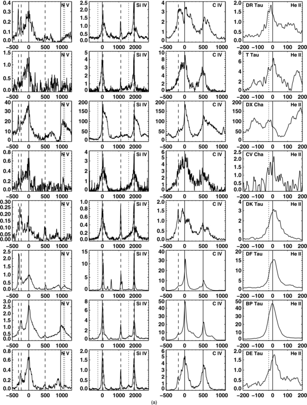
Download figure:
Standard image High-resolution image
Download figure:
Standard image High-resolution image
Download figure:
Standard image High-resolution image
Figure 14. Hot lines for CTTSs ordered by decreasing  . Left to right: N v, Si iv, C iv, He ii. The plots show flux density (10−14 erg s−1 cm−2 Å−1) vs. velocities (km s−1) in the stellar rest frame. The spectra are not extinction-corrected nor continuum-subtracted. Transition disks are indicated with "TD" after the name. Solid lines: nominal line positions; dashed lines: nominal locations of the strongest H2 lines. N v, dotted lines: N i (1243.18 Å, +1055 km s−1; 1243.31 Å, +1085 km s−1). Si iv, dotted lines: CO A-X (5–0) bandhead (1392.5 Å, −271 km s−1), O iv (1401.17 Å, +1633 km s−1). He ii, dotted line: location of the secondary He ii line (Section 6).
Download figure:
Standard image High-resolution image
Figure 15. The "hot" lines for WTTS. The stars are listed in alphabetical order. Axes and markings are the same as in Figure 14.
Download figure:
Standard image High-resolution image
Figure 16. Both members of the C iv doublet, scaled and overplotted. The 1550 Å line (the red member of the doublet) is shown in red, and it has been scaled to match the red wing of the 1548 Å line. Axes and units are the same as in Figure 14.
Download figure:
Standard image High-resolution image
Figure 17. The black trace shows the He ii line overplotted to the 1550 Å C iv and scaled to the same maximum value. Axes and units are the same as in Figure 14.
Download figure:
Standard image High-resolution image
Footnotes
- 18
We refer to the overall sample of accreting objects as the "CTTSs sample," in spite of the inclusion of this Herbig Ae star.
- 19
The p-value is the probability of obtaining a value of the test statistic at least as extreme as the observed one, assuming the null hypothesis is true. In this case, it is the probability that the Pearson's r is as large as measured or larger, if the two quantities are uncorrelated. We reject the null hypothesis if p-value ⩽0.05.
- 20
We note that for HN Tau A, the radial velocity (4.6 ± 0.6 km s−1), derived by Nguyen et al. (2012), which we use here, deviates significantly from the velocity of the surrounding molecular cloud (21 km s−1; Kenyon & Hartmann 1995). Using the cloud velocity would shift the C iv lines to the blue even more. France et al. 2012 finds that the H2 lines have maxima at ∼20 km s−1 from the rest velocity, although the line asymmetry suggest components at lower velocity.
- 21
In their published analysis, France et al. (2010) fit the C iv lines of 2M1207 with two Gaussian components each. However, that analysis is based on an early reduction of the COS data. A new re-processing and new Gaussian decomposition shows that the C iv line can be fit with one Gaussian component (K. France 2013, private communication).