


ABSTRACT
We present a new catalog of spectroscopically confirmed white dwarf stars from the Sloan Digital Sky Survey (SDSS) Data Release 7 spectroscopic catalog. We find 20,407 white dwarf spectra, representing 19,712 stars, and provide atmospheric model fits to 14,120 DA and 1011 DB white dwarf spectra from 12,843 and 923 stars, respectively. These numbers represent more than a factor of two increase in the total number of white dwarf stars from the previous SDSS white dwarf catalogs based on DR4 data. Our distribution of subtypes varies from previous catalogs due to our more conservative, manual classifications of each star in our catalog, supplementing our automatic fits. In particular, we find a large number of magnetic white dwarf stars whose small Zeeman splittings mimic increased Stark broadening that would otherwise result in an overestimated log g if fit as a non-magnetic white dwarf. We calculate mean DA and DB masses for our clean, non-magnetic sample and find the DB mean mass is statistically larger than that for the DAs.
Export citation and abstract BibTeX RIS
1. INTRODUCTION
The Sloan Digital Sky Survey (SDSS; York et al. 2000) has had impacts in astronomy far beyond its main mission of exploring the three-dimensional structure of our universe. The Sloan Extension for Galactic Exploration and Understanding survey (SEGUE; Lee et al. 2008), part of the second-generation SDSS surveys, extended the survey's mission to unraveling the nature and structure of our own Milky Way galaxy by targeting mostly new fields in and around the Galactic disk. As a result, the spatial distribution of the new (largely Galactic disk) white dwarf stars in this catalog will be very different from those in the earlier catalogs from SDSS Data Release 1 (DR1; Kleinman et al. 2004) and Data Release 4 (DR4; Eisenstein et al. 2006a) where the focus was on extragalactic objects and the Galactic disk was purposefully avoided. The study of white dwarf stars has benefited greatly from the increased number of objects provided by the SDSS, there being 66 papers between 2005 and 2012 reported by the SAO/NASA Astrophysics Data System, for example, with "SDSS" and "white dwarf" in the title. Numerous other papers refer to SDSS-discovered white dwarf stars without indicating so in the title. The first full white dwarf catalog from SDSS data (Kleinman et al. 2004), based on SDSS DR1 (Abazajian et al. 2003), roughly doubled the number of then known white dwarf stars. Using data from the SDSS DR4 (Adelman-McCarthy et al. 2006), Eisenstein et al. (2006a) reported over 9000 spectroscopically confirmed white dwarf stars from the SDSS, again roughly doubling the combined number of white dwarf stars known after SDSS DR1. With the release of Data Release 7 from the SDSS (DR7; Abazajian et al. 2009), we again roughly double the number of identified white dwarf stars compared to those in the DR4 sample.
The first release of SEGUE data started in SDSS Data Release 6 (Adelman-McCarthy et al. 2008), with more released in SDSS DR7 (Abazajian et al. 2009). In the original SDSS survey, white dwarf spectra were obtained primarily as a bi-product of other high-priority categories of targets. Almost all were hot white dwarf stars because white dwarf stars cooler than ≈7000 K have colors similar to the more numerous FGK main-sequence stars which were specifically not targeted. Most of the white dwarf stars in the survey were not targeted for spectroscopy as white dwarf star candidates and were instead rejects from targeting algorithms for other kinds of objects; Kleinman et al. (2004) and Harris et al. (2003) discuss the details of the DR1 target selection and the makeup of the white dwarf spectroscopic sample. The SEGUE survey, however, specifically targets stars (see http://www.sdss3.org/dr8/algorithms/segueii/segue_target_selection.php) and cool white dwarf stars were effectively targeted for the first time using their reduced proper motions. The net result is that the number of white dwarf stars observed per SDSS spectroscopic plate has remained roughly constant at 25/plate through each SDSS Data Release, although the selection mechanism is significantly different.
Here, we report on the white dwarf catalog built from the SDSS DR7. We have applied automated techniques supplemented by complete, consistent human identifications of each candidate white dwarf spectrum. We make use of the latest SDSS reductions and white dwarf model atmosphere improvements in our spectral fits, providing log g and Teff determinations for each identified clean DA and DB where we use the word "clean" to identify spectra that show only features of non-magnetic, non-mixed, DA or DB stars. Our catalog includes all white dwarf stars from the earlier Kleinman et al. (2004) and Eisenstein et al. (2006a) catalogs, although occasionally with different identifications, as discussed below.
Looking for infrared excesses around DA white dwarf stars, Girven et al. (2011) use a photometric method to identify DA white dwarf stars with g < 19 from the SDSS and find 4636 spectroscopically confirmed DAs in DR7 with another 5819 expected DAs in the photometric sample. Our sample is not magnitude-selected (although classifications typically get more uncertain for g ≈ 19.5 and below) and includes DB and all other white dwarf subtypes as well. We do not, however, consider candidate white dwarf stars that do not have SDSS spectra.
We note that although we did not fit white dwarf plus main-sequence models to our apparently composite spectra, others (Silvestri et al. 2006; Marsh et al. 2011; Girven et al. 2011; Koester et al. 2011; Debes et al. 2011; Steele et al. 2011; Rebassa-Mansergas et al. 2012) have specifically studied these spectra.
2. CANDIDATE SELECTION
SDSS DR7 contains over 1.6 million spectra and we did not have the facilities to fit and identify each spectrum. We therefore had to extract a smaller subsample of candidates from these spectra that we could later fit and examine as possible white dwarf stars. To form our candidate sample, we employed two different techniques. First, we reproduced the candidate selection from Eisenstein et al. (2006a), but implemented it completely within the SDSS DR7 Catalog Archive Server (CAS)10 as an SQL query. This query returned 24,189 objects.
Second, we used the SDSS and SEGUE target classification and spectrum analysis fields and selected any object that was either targeted as a possible white dwarf star or whose spectrum was determined to likely be any kind of white dwarf star. This query returned 48,198 spectrum IDs. Both queries are listed in full in the Appendix and queried all available DR7 spectra via the specObjAll table.
Combined, these queries resulted in 53,408 unique spectra, of which 5209 uniquely satisfied the Eisenstein et al. (2006a) criteria, 29,218 uniquely satisfied the new target/classification criteria, and 18 981 spectra satisfied both. Later, we discovered that 4362 sky spectra made our sample (they should have been explicitly excluded from our queries, but were not), so these were deleted and the resulting sample size became 49,046 spectra. Ultimately, 4% of the objects which were selected only by the targeting criteria, 36% of those selected only by the Eisenstein et al. (2006a) criteria, and 90% of those that satisfied both criteria were labeled as white dwarf stars. The combined set of criteria is a very powerful way to identify white dwarf spectra in the SDSS, accounting for 83% of our identified white dwarf stars. Only 17% of the identified white dwarf stars, therefore, satisfied just one of the two selection criteria.
We further pared our sample by using lists of previously identified SDSS spectra. We removed the known quasars (Schneider et al. 2010), BL Lac objects (Plotkin et al. 2010), and once we had run through our DA and DB model-fitting program, we fit the rejects with galaxy and quasar templates (Yip et al. 2004a, 2004b) to remove these objects from further consideration. This process removed an additional 6892 spectra, resulting in a final sample of 42,154 spectra.
3. WHITE DWARF ATMOSPHERE MODELS
The mechanics of our autofit fitting program, which fits the observed spectra to our synthetic model spectral grid by χ2 minimization, remain the same as described in Kleinman et al. (2004) and Eisenstein et al. (2006a), but substantial improvements have been made to our atmospheric model grid, both in the model physics and the parameters of the grid itself.
We use updated Koester (Koester et al. 2009a; Koester 2010) model atmospheres, with the following significant changes since Kleinman et al. (2004).
- 1.
- 2.The Stark broadening profiles from Beauchamp et al. (1997) for hydrogen have been convolved with the neutral broadening profiles to add another dimension for the neutral particle density to the broadening tables. For the three lowest Balmer lines, we used the self-broadening data of Barklem et al. (2000). For the higher series members, we used the sum of resonance (Ali & Griem 1965) and van der Waals broadening (Unsöld 1968). For the helium lines, we used self-broadening data from Leo et al. (1995) and Mullampht et al. (1991). For the remaining lines, simple estimates for resonance and van der Waals broadening were used.
- 3.The Holtsmark microfield distribution was replaced by the Hooper (1966, 1968) distribution using the approximations in Nayfonov et al. (1999). This distribution includes correlations between the charged perturber particles. The changes in the occupation probabilities for higher Balmer lines, where the occupation probability varies between 0.1 and 1.0, are quite significant.
- 4.For the DBs, we now use the ML2/α = 1.25 approximation. We find that this value best describes the location of the DBV instability strip (Montgomery 2007; Corsico et al. 2009; Montgomery et al. 2010). Montgomery et al. (2010), in particular, exclude values of α < 0.8 through their analysis of the convection zone for the pulsating DB white dwarf, GD 358 while Bergeron et al. (2011) justify this value in their atmospheric modeling.
- 5.For the DAs, we use ML2/α = 0.6. Note that with the use of these improved Stark profiles, Tremblay et al. (2010) showed that a slightly more efficient convective energy transport with α = 0.8 should be used, although we feel our atmospheric parameters with α = 0.6 are appropriate in the present context.
Our model grid now extends to log g = 10.0 and is denser than that used in Eisenstein et al. (2006a) and Kleinman et al. (2004). For DAs, the grid extends in log g from 5.0 to 10.0 in steps of 0.25 while Teff goes from 6000 K to 10,000 K in steps of 250 K, 10,000 K to 14,000 K in steps of 100 K, 14,000 K to 20,000 K in steps of 250 K, 20,000 K to 50,000 K in steps of 1000 K, and 50,000 K to 100,000 K in steps of 2500 K. The DB grid runs from log g = 7.0 to 10.0 in steps of 0.25, with Teff extending from 10,000 K to 18,000 K in steps of 250 K and from 18,000 K to 50,000 K in steps of 1000 K.
4. SPECTRAL FITTING
Once we completed our candidate list, we fit all 42,154 candidate white dwarf spectra and colors with our autofit code described in Kleinman et al. (2004) and Eisenstein et al. (2006a). Autofit fits only clean DA and DB models, so does not recognize other types of white dwarf stars. In addition to the best-fitting model parameters, it also outputs a goodness-of-fit estimate and several quality control checks and flags for other features noted in the spectrum or fit.
We took the output from autofit and separated the results into good DA and DB fits (14,271 spectra) and all else (27,883 spectra). We looked at all the good DA and DB fits to verify they were indeed normal DAs and DBs and made about 1000 ID changes. In almost all cases, we agreed each spectrum was one of a DA or DB white dwarf star, but found they also contained additional spectral features not fit by our models, resulting in new identifications like DAB, DAH, DA+M, etc. We also looked at each spectrum autofit failed to classify as a DA or DB dwarf star, identifying some as other white dwarf subtypes while most were simply other non-white-dwarf stellar spectra.
4.1. Spectral Classification
Since autofit can only classify clean DA and DB spectra, we knew we would have to look at its rejected spectra for other white dwarf spectral types. Because we were interested in obtaining accurate mass distributions for our DA and DB stars, we were conservative in labeling a spectrum as a clean DA or DB. That is, we were liberal in adding additional subtypes and uncertainty notations if we saw signs of other elements, companions, or magnetic fields in the spectra. While some of our mixed white dwarf subtypes would probably be identified as clean DAs or DBs with better signal-to-noise (S/N) spectra, few of our identified clean DAs or DBs would likely be found to have additional spectral features within our detection limit.
To aid searching for other white dwarf subtypes beyond the DAs and DBs, we selected all objects that had not been successfully fitted as a DA or DB star by autofit and then further selected only those with (g − r) < 0.5, (u − g) < 0.8, and g < 19.5. The color cuts helped to limit interlopers since most white dwarf stars fall within these ranges and the magnitude cut simply helps ensure a S/N high enough to allow spectral identification. We thus obtained a list of 7864 objects that were then spectrally classified as discussed below. In general, we looked for the following features to aid in the classification for each specified white dwarf subtype.
- 1.Balmer lines—normally broad and with a Balmer decrement (DA but also DAB, DBA, DZA, and subdwarfs).
- 2.He i 4471 Å (DB, subdwarfs).
- 3.He ii 4686 Å (DO, PG1159, subdwarfs).
- 4.C2 Swan band or atomic CI lines (DQ).
- 5.Ca ii H and K (DZ, DAZ).
- 6.CII 4367Å (HotDQ).
- 7.Zeeman splitting (magnetic DA)
- 8.Featureless spectrum with significant proper motion (DC).
- 9.Flux increasing in the red (binary, most probably M companion).
Many of the stars analyzed in this way turned out to be genuine DA or DB white dwarf stars that had been rejected by autofit for lack of S/N, too many bad pixels in the spectra, uncertain colors, etc. Many were also multi-subtype white dwarf stars like DAH, DBA, DAZ, DBZ or DA+M and DB+M.
We found many objects with both strong Balmer lines and He i lines. These objects are likely double-degenerate binaries composed of a DA and a DB white dwarf, but following standard nomenclature, we simply classified them as DAB or DBA, as appropriate. Another group of objects had Balmer lines less deep than what is expected for DA white dwarf stars with their derived effective temperatures. These stars are also most likely double degenerates consisting of a DA and a DC white dwarf star, but were classified as DAs. Tremblay et al. (2011) analyze these potential double degenerates.
We also found a group of stars to have a very steep Balmer decrement (i.e., only a broad Hα and sometimes Hβ is observed while the other lines are absent) that could not be fit with a pure hydrogen grid. We find that these objects are best explained as helium-rich DAs, as confirmed by fits with a grid of helium-rich white dwarf stars with traces of hydrogen (see Dufour et al. 2007a). These white dwarf stars are most probably former DZAs where all the metals have gravitationally settled while the hydrogen still floats at the surface.
For the other spectral types (DC, DZ, DQ and HotDQ), we used an appropriate grid and fitted the spectroscopic and photometric data (see Dufour et al. 2005, 2007a, 2007b; Koester & Wilken 2006; Dufour et al. 2008 for details) to confirm the classification. Objects that could not be fitted using one of the grids were thus easily spotted and put in the non-white dwarf category.
We finally note that the white dwarf color space also contains many hot subdwarfs. It is difficult, just by looking at a spectrum, to tell a low-mass white dwarf from a subdwarf. To guide us in the classification of hot stars, we superposed over the observed spectra a log g = 7 model at the effective temperature given by a fit to the ugriz colors. We then rejected objects showing lines much less broad than the synthetic spectrum. We also declared a subdwarf to be anything labeled as a subdwarf ("SD"), DB, or DA by our autofit code with a log g of 6.5 or less and human-classified as either a subdwarf or a DA or a DB. Since the autofit-measured values of Teff and log g are not reliable for anything other than a clean DA/DB spectrum, anything that passed the autofit subdwarf criteria but was human-classified as anything other than a subdwarf or clean DA/DB was not classified as a subdwarf. So, for example, some DAMs in our catalog that have low autofit log g values may actually be subdwarf + M systems.
4.2. Classification Results
Table 1 lists the number of each type of white dwarf star we identified. Table 2 lists the columns of data provided in our electronic catalog file (in comma separated variable format). The full catalog is available in the online version of the journal.
Table 1. Numbers of Identified White Dwarf Types
| No. of Stars | No. of Spectra | Type |
|---|---|---|
| 12 843 | 14 120 | DAs |
| 923 | 1011 | DBs |
| 628 | 681 | DAH |
| 10 | 22 | DBH |
| 91 | 101 | Other magnetic |
| 559 | 605 | DC |
| 409 | 447 | DZ |
| 220 | 243 | DQ |
| 61 | 65 | DO/PG 1159 |
| 1735 | 1951 | WD+MSa |
| 124 | 141 | WDmixb |
| 951 | 1020 | WDuncc |
Notes. aThese spectra show both a white dwarf star and a companion, non-white dwarf spectrum, usually a main-sequence M star. bThese stars are mixed white dwarf subtypes. We did not attempt to resolve if the observed features resulted from single star or multiple star systems. cThese spectra were identified as uncertain white dwarf stars.
Download table as: ASCIITypeset image
Table 2. Columns Provided in Data Tables
| Column No. | Heading | Description |
|---|---|---|
| 1 | Name | SDSS object name (SDSS 2000J+) |
| 2 | Plate | SDSS plate number |
| 3 | MJD | SDSS Modified Julian date |
| 4 | Fiber | SDSS FiberID |
| 5 | RA | Right ascension |
| 6 | Dec | Declination |
| 7 | SN_g | SDSS g-band signal-to-noise ratio |
| 8 | u_psf | SDSS u-band PSF magnitude |
| 9 | u_err | SDSS u-band PSF magnitude uncertainty |
| 10 | u_flag | SDSS u-band quality control flaga |
| 11 | g_psf | SDSS g-band PSF magnitude |
| 12 | g_err | SDSS g-band PSF magnitude uncertainty |
| 13 | g_flag | SDSS g-band quality control flaga |
| 14 | r_psf | SDSS r-band PSF magnitude |
| 15 | r_err | SDSS r-band PSF magnitude uncertainty |
| 16 | r_flag | SDSS r-band quality control flaga |
| 17 | i_psf | SDSS i-band PSF magnitude |
| 18 | i_err | SDSS i-band PSF magnitude uncertainty |
| 19 | i_flag | SDSS i-band quality control flaga |
| 20 | z_psf | SDSS z-band PSF magnitude |
| 21 | z_err | SDSS z-band PSF magnitude uncertainty |
| 22 | z_flag | SDSS z-band quality control flaga |
| 23 | PM | SDSS proper motion (0.01 arsec yr−1) |
| 24 | PM_angle | SDSS proper motion angle (+north through east) |
| 25 | PM_match | SDSS proper motion match (1 = successful match within 1.0 arsec) |
| 26 | A_g | SDSS g-band extinction |
| 27 | GMT | SDSS mjd_r (GMT when row 0 of r measurement read) |
| 28 | AutoType | autofit ID |
| 29 | T_eff | autofit Teff |
| 30 | T_err | autofit Teff uncertainty |
| 31 | log_g | autofit log g |
| 32 | log_gerr | autofit log g uncertainty |
| 33 | chisq | autofit χ2 fit measurement |
| 34 | uniq | unique numberb |
| 35 | Mass | Calculated mass for clean DAs and DBs only |
| 36 | Mass_err | Mass uncertainty |
| 37 | humanID | Human ID assigned this spectrum |
aThe photometric flag values are processed versions of the flagsband parameter in the SDSS database. It has been logically anded with the appropriate values to highlight objects that have the following quality control flags set: EDGE, PEAKCENTER, NOPROFILE, BAD_COUNTS_ERROR, INTERP_CENTER, DEBLEND_NOPEAK, PSF_FLUX_INTERP, SATURATED, and NOTCHECKED. If the value is non-zero, then the corresponding SDSS magnitude is suspect. bThe unique number is assigned to identify duplicate spectra of the same object. For objects with only one spectrum, the value of this column is uniq. For objects with more than one spectrum, the value will be dup-xxxx where xxxx is a running number, the same for all spectra of the same object. The spectrum with the highest signal-to-noise ratio for objects with duplicate spectra will be identified with an a at the end of its dup-xxxx name.
Only a portion of this table is shown here to demonstrate its form and content. A machine-readable version of the full table is available.
Download table as: DataTypeset image
5. SAMPLE COMPLETENESS
As discussed in the Kleinman et al. (2004) and Eisenstein et al. (2006a) catalogs, the spectroscopic sample of white dwarf stars from the SDSS is not at all complete. That is, not every white dwarf star in the SDSS photometric survey has a corresponding SDSS spectrum. There are many complex biases and selection effects based on the many different criteria used to obtain these white dwarf spectra. Each individual criterion has a different priority when it comes to designating objects in a given part of the sky for follow-up spectroscopy, Since the selection criteria, weights, and biases, however, are all known, the completeness of our spectroscopic white dwarf sample is knowable, but is beyond the focus of this work.
Since we did not look at, or even fit, every SDSS spectrum in DR7, we do need to estimate how complete our catalog is compared to the overall, but unknown, SDSS spectroscopic white dwarf sample. Did we recover every white dwarf with a spectrum in DR7? One way we can address this question is to see how many of the Kleinman et al. (2004) and Eisenstein et al. (2006a) white dwarf stars we recovered in our new catalog since our candidate selection and fitting were done independently of the earlier catalogs.
When comparing our catalog with Table 11 from Eisenstein et al. (2006a), we found 241 missing out of 10,090 objects or about 2.4%. We then added the missing spectra to our candidate list and proceeded to analyze them along with the rest of our candidates. A spot check of these objects showed that they do not pass the color cuts described in Section 3.1 of Eisenstein et al. (2006a) in either the SDSS DR4 or DR7 database. Eisenstein et al. (2006a) used some preliminary photometry in the early candidate selection process and did not redo the candidate selection once the released DR4 photometry became available, so this likely explains why we did not pick them up in our candidate list. The completeness of this catalog, therefore, ought to be at least as good as that of Eisenstein et al. (2006a).
Doing a similar test with Table 5 from Kleinman et al. (2004) resulted in 258 white dwarf stars from the DR1 catalog not making our candidate list. Fifty-three of them belong to Plate–MJD pairs which are not part of DR7 and 72 stars were the same as those missing from the Eisenstein et al. (2006a) DR4 catalog. So, combined, there were 183 out of 2971 stars from the DR1 catalog, or ≈6% not included in either our original candidate list or in the DR4 catalog. The candidate selection parameter space in the DR1 catalog (Kleinman et al. 2004), though, was much more extensive than that used in the DR4 catalog (Eisenstein et al. 2006a), and thus, here so that missing parameter space, if included here, would probably result in another 600 or so white dwarf stars, most of which would be cooler and overlap the A and F main-sequence star region.
5.1. Literature Comparison
Figure 1 shows the comparison for 195 DAs and 10 DBs between our autofit determinations and those in the literature (Oke et al. 1984; Finley et al. 1997; Friedrich et al. 2000; Claver et al. 2001; Gianninas et al. 2005; Liebert et al. 2005; Lisker et al. 2005; Kawka & Vennes 2006; Kepler et al. 2006; Voss et al. 2007; Kilic et al. 2007; Lajoie & Bergeron 2007; Stroeer et al. 2007; Holberg et al. 2008; Gänsicke et al. 2008; Nebot Gómez-Morán et al. 2009; Pyrzas et al. 2009; Allende Prieto et al. 2009; Kilic et al. 2010; Girven et al. 2010; Kulkarni & van Kerkwijk 2010). We have not included in the comparison the values from DR1 or DR4. The figure clearly shows that our fit parameters are generally in very good agreement with those from the literature, where overlap does occur.

Figure 1. Comparisons of our autofit version auto32 fits to atmospheric values in the literature. The diagonal line shows the one-to-one correspondence. The black circles are DAs and the blue squares, DBs. The larger scatter seen above Teff ≈ 50, 000 K is due to our models assuming local thermodynamic equilibrium (LTE) whereas non-LTE (NLTE) models are needed for these temperatures.
Download figure:
Standard image High-resolution imageGianninas et al. (2011) obtained S/N ⩾ 50 spectra of 177 white dwarfs in common with our sample and estimated Teff and log g values for those using the Montreal group atmospheres with ML2/α = 0.8 convection theory, fitting the line profiles only. In Figure 2, we plot their determinations and ours for the 162 white dwarfs that do not show a companion in our spectra. The agreement is good in spite of the different spectra, different models, and different fitting procedures. For stars hotter than Teff ≈ 50, 000 K the differences are larger because our models assume local thermodynamical equilibrium (LTE).

Figure 2. Comparisons of our autofit fits to atmospheric values in Gianninas et al. (2011).
Download figure:
Standard image High-resolution image5.2. Consistency
Before rationalizing our identifications and removing the subdwarf spectra, we found 1683 objects in our catalog with more than one spectrum in DR7. There are a total of 3591 spectra for these 1683 objects, so most duplicates have only two spectra in total. Two objects have seven DR7 spectra, the most of all the duplicates. Each duplicate spectrum was independently fit by autofit and by eye so we could use the duplicate IDs as a consistency check to our results. Figure 3 shows the resulting comparison from our autofit results. The average absolute value of the difference in Teff is 680 K and the average absolute value of the difference in log g is 0.16.
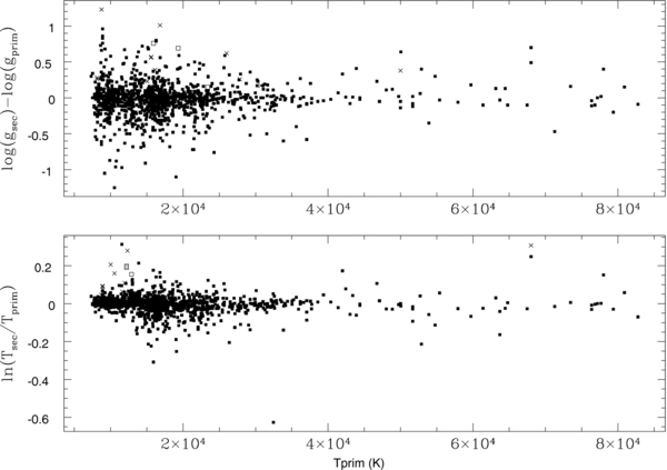
Figure 3. autofit comparisons of fits to duplicate spectra of clean DA and DB white dwarf stars in our catalog. Solid squares represent objects where the duplicate measurements differ by less than 3σ, the ×'s between 3σ and 5σ, and the hollow squares >5σ.
Download figure:
Standard image High-resolution imageOf the set of 3591 duplicate spectra, only 242 of them had human identifications that disagreed with each other. Two hundred and twelve of these agreed in the dominant subtype with 13 differing only by our uncertainty note, a ":", indicating an uncertain identification of the indicated spectral feature. One hundred and forty-one identifications differed by an additional subtype or a subtype and a ":", and 58 differed by more than one subtype. The remaining 30 identifications, ≈0.8% of the sample, disagreed in dominant subtype and are mostly DAB/DBA, DA/DC, and DA/SDB pairs. We examined each one of these disagreeing IDs and selected the best identification (usually that of the highest S/N spectrum) and applied it to all spectra for each object. In general, we found our classifications were different only for low S/N spectra.
We also compared our identifications with those made in the Eisenstein et al. (2006a) DR4 catalog. Of the 10,090 WDs in the DR4 catalog, 8527 of our IDs agreed; 1563 of them disagreed. Of these 1563 disagreements, 1330 agreed in dominant subtype, with 254 differing only by a ":", 591 by an additional subtype or a subtype and a ":", and 485 by more than one subtype. Two hundred and twenty-seven, ≈2%, disagree in dominant subtype. Eisenstein et al. (2006a) did not hand-identify each object in the catalog, relying on autofit to accurately report clean DA and DBs and to identify which subset of objects to look at individually. Thus, this level of disagreement between our two catalogs seems consistent with our 100% hand-checked identifications.
Comparisons of our autofit parameters of the DR4 stars in DR7 with the DR4 fits is a measure of the changes to both our autofit models and the DR7 SDSS spectral reductions. Figures 4 and 5 show the DA and DB log g and Teff distributions for the DR7 objects in DR4. The biggest changes occur at the cool end of the DA distribution where the DR4 fit values rise to higher log g with lower Teff, a change due to the improved input model neutral broadening physics discussed earlier. Our new model grid's increase in range in log g and Teff is also clearly evident in these figures.

Figure 4. Comparison of DA log g vs. Teff autofit values for DR4 stars also in DR7. The top panel shows the DR4 values while the bottom panels show our new determinations. Our improved model physics have reduced the rise to higher log g at lower temperatures to a bump, improving, but not completely eliminating this well-known model artifact (e.g., Tremblay et al. 2010).
Download figure:
Standard image High-resolution image
Figure 5. Comparison of DB log g vs. Teff autofit values for DR4 stars also in DR7. The top panel shows the DR4 values while the bottom panels show our new determinations.
Download figure:
Standard image High-resolution image6. RESULTS
Besides producing the catalog itself, which we hope will spawn many future papers and much analysis, we report here on the increased number of magnetic white dwarf stars found in this catalog, compared with those previous. We also look at the mass distribution of our DA and DB samples and find a decidedly non-Gaussian DA mass distribution and a statistically significant difference in mean mass between the DAs and the DBs. As in Eisenstein et al. (2006a) and Eisenstein et al. (2006b), we again find no statistically significant DB gap.
6.1. Magnetic Fields and Zeeman Splittings
When examining each candidate spectrum, we found hundreds of stars with Zeeman splittings indicating magnetic fields above 3 MG (the limit below which we do not think we can accurately identify) that if not identified as magnetic in origin, would have rendered inaccurate autofit Teff and too high log g determinations. We ended up classifying 628 DAHs, 10 DBHs, and 91 mixed atmosphere magnetics, compared to only 60 magnetic white dwarf stars of all types identified in Eisenstein et al. (2006a).
Schmidt et al. (2003) found 53 magnetic white dwarf stars in DR1 and Vanlandingham et al. (2005) found 52 in DR3 data. Most of these stars did not make the Eisenstein et al. (2006a) DR4 catalog because they did not meet the candidate selection criteria.
We also identified several hundred possible magnetic stars with low S/N spectra that made solid identifications difficult. These objects are accounted for in the WDunc category in Table 1. Wishing to not bias our mass distribution with a magnetic sample, we chose to label them uncertain magnetic (DH:) stars since even fields as low as ≈3 or more MG will affect autofit gravity determinations substantially.
Külebi et al. (2009) independently found 44 of our newly classified magnetic DAs and fitted the SDSS spectra to atmospheric models including off-centered dipoles, assuming log g = 8.
Here, we are reporting the number of magnetic white dwarfs stars relative to those non-magnetic to be roughly 3.5%. This number is in reasonable agreement with Schmidt & Smith (1995), for example, but is significantly larger than the ≈0.1% and 1.5% reported in the DR4 (Eisenstein et al. 2006a) and DR1 (Kleinman et al. 2004) catalogs, respectively. The DR4 catalog was based primarily on computer identifications, supplemented by only partial human checks, thereby explaining part of the reason for the lower numbers of magnetic white dwarf identifications in Eisenstein et al. (2006a). Beyond this cause, however, the algorithm we used to manually identify possible magnetic white dwarf stars developed significantly since the DR1 and DR4 catalogs. Combined with our desire to develop a clean sample for mass estimation, we ended up with the larger, though plausible, percentage gain of magnetic white dwarf stars seen here.
To validate our identification methods, we conducted several blind simulations where we hand-identified model spectra with varying amounts of added noise and magnetic field strength (from 0 to 800 MG). These simulations are reported in more detail in Kepler et al. (2012), but the summary result is that our human identifications were proven valid for spectra with S/N > 8 and B > 2MG. In addition, at the very largest magnetic field strengths, we found we are not identifying all the magnetic white dwarf stars, instead labeling them as unknown stars or sometimes, DC. Figure 6 shows the percentage of identified magnetic DA white dwarf stars as a function of spectral S/N and Figure 7 shows the absolute number of DAH identifications per S/N bin. These plots suggest that below S/N < 8, at least half of our ≈280 DAH identifications are likely magnetic and that spectra below ≈S/N < 8 ought to be confirmed with higher S/N and possibly higher resolution spectra before declaring them magnetic or not.

Figure 6. Percentage of identified magnetic white dwarf spectra as a function of spectral signal to noise.
Download figure:
Standard image High-resolution image
Figure 7. Number of identified DAH stars as a function of spectral signal to noise.
Download figure:
Standard image High-resolution image6.2. Mean Masses
To calculate the mass of our identified clean DA and DB stars from the Teff and log g values obtained from our fits, we used the mass–radius relations of Renedo et al. (2010) for carbon–oxygen DA white dwarfs. These relations are based on full evolutionary calculations appropriate for the study of hydrogen-rich DA white dwarfs that take into account the full evolution of progenitor stars from the zero-age main sequence through the core hydrogen-burning phase, the helium-burning phase, and the thermally pulsing asymptotic giant branch phase. The stellar mass values of the resulting sequences are: 0.525, 0.547, 0.570, 0.593, 0.609, 0.632, 0.659, 0.705, 0.767, 0.837, and 0.878 M☉. These sequences are supplemented by sequences of 0.935 and 0.98 M☉ calculated specifically for this work. For high-gravity white dwarf stars, we employed the mass–radius relations for oxygen/neon core white dwarf stars given in Althaus et al. (2005) in the mass range from 1.06 to 1.36 M☉ with a step of 0.02 M☉. For the low-gravity white dwarf stars, we used the evolutionary calculations of Althaus et al. (2009b) for helium-core white dwarf stars. These sequences are characterized by stellar mass values of 0.22, 0.25, 0.303, 0.40, and 0.452 M☉. They were complemented with the sequences of 0.169 and 0.196 M☉ taken from Althaus et al. (2010).
For DB white dwarf stars, we relied on the evolutionary calculations of hydrogen-deficient white dwarf stars of 0.515, 0.530, 0.542, 0.565, 0.584, 0.609, 0.664, 0.741, and 0.870 M☉ computed by Althaus et al. (2009a). These sequences constitute an improvement over previous calculations. In particular, they have been derived from the born-again episode responsible for the hydrogen deficiency. For high-gravity DBs, we used the oxygen/neon evolutionary sequences described above for the case of a hydrogen-deficient composition.
These evolutionary sequences constitute a complete and homogeneous grid of white dwarf models that captures the core features of progenitor evolution, in particular the internal chemical structures expected in the different types of white dwarf stars.
To calculate reliable mass distributions, we selected only the best S/N spectra with temperatures well fit by our models. We find reliable classifications can be had from spectra with S/N ⩾ 15, in agreement with Tremblay et al. (2011). We classified 14,120 spectra as clean DAs, but selecting the highest S/N spectra for those with duplicate spectra, we are left with 12,813 clean DA stars. Of these DAs, 3577 have a spectrum with S/N ⩾15, with a mean S/N = 25 ± 10. Using this sample, we obtain 〈MDA〉 = 0.623 ± 0.002 M☉.
This mean mass estimate is incorrect, however, if we believe the apparent increase in fit log g at low Teff is an artifact of our models and not inherent in the stars. Although Liebert et al. (2003), Kepler et al. (2007, 2010), Tremblay et al. (2011), and Gianninas et al. (2011) all show an increase in measured log g for DAs with measured temperatures of order 12,000–13,000 K or less, this increase is probably due to missing physics in the models and not due to the stars, since the photometric determinations and gravitational redshifts (Koester & Knist 2006; Falcon et al. 2010) do not show this log g increase.
We therefore further restricted our sample to those DAs with a measured Teff > 13, 000 K, and from a sample of now 2217 objects, we determined 〈MTeff > 13, 000KDA〉 = 0.593 ± 0.002 M☉.
Our mean DA mass is smaller than that of Tremblay & Bergeron (2009), even though we are using the same Stark broadening and microfield as they are. Our sample is five times larger, however, and we have removed suspected magnetic DAs from our sample, which would otherwise increase our measured mean mass. Limoges & Bergeron (2010), with the same models as Tremblay & Bergeron (2009), obtained a mean mass of 0.606 ± 0.135 M☉ for their KISO survey DA sample, and 0.758 ± 0.192 M☉ for their DB sample. Falcon et al. (2010) determined the mean ensemble mass of a sample of 449 DAs observed in the ESO SN Ia progenitor survey (SPY) project, using their mean gravitational redshift and found 〈M〉 = 0.647 ± 0.014 M☉, a value substantially higher than ours. This value is independent of the line profiles themselves and therefore should not be affected by linear magnetic field effects. At the resolution of the SPY data (Koester et al. 2001), Koester et al. (2009b) were able to identify fields larger than 90 kG, so the contribution of nonlinear magnetic effects should also be negligible. Gianninas et al. (2011), using ML2/α = 0.8 models, find 〈M〉 = 0.638 M☉ by fitting line profiles for high S/N spectra for stars hotter than Teff = 13, 000 K. Romero et al. (2012) also report a mean mass of 0.636 M☉ for their asteroseismological analysis of 44 bright pulsating DA (ZZ Ceti, or DAV) stars.
If ≈10% of our S/N > 15, Teff > 13, 000 K stars were non-magnetic with masses of order 0.9 M☉, our mean DA mass would rise to ≈0.63 M☉, more consistent with previous measurements. Such a number, though, would require all our identified magnetic stars, and then some, to be both massive and non-magnetic, so our lower mass estimate can be only partially explained by our magnetic white dwarf identifications. Additionally, we note that the Tremblay et al. (2011) re-analysis of the DR4 white dwarf stars resulted in a measurement of 〈MDA〉 = 0.613 M☉, again lower than most previous studies and similar to our new measurement.
The 1011 spectra we classified as clean DBs belong to 923 stars. One hundred and ninety-one of these have a spectral S/N ⩾15, with a mean S/N = 23 ± 7. Using this high S/N sample, we obtain 〈MDB〉 = 0.685 ± 0.013 M☉. Restricting this sample to just those hotter than Teff = 16, 000 K, again assuming the increase in measured log g seen below this temperature is an artifact of the models and not inherent to the stars, we obtain 140 stars, resulting in 〈MTeff > 16, 000KDB〉 = 0.676 ± 0.014 M☉. The masses of DAs and DBs are therefore statistically different, as also found by Kepler et al. (2007), Tremblay et al. (2010), and Bergeron et al. (2011). This difference is consistent with the possibility that DBs come through a very late thermal pulse phase, which burns the remaining surface H after reaching the white dwarf cooling phase. Figure 8 shows the obtained mass histograms for our final DA and DB samples.

Figure 8. Histogram of the masses for S/N ⩾ 15 clean DAs (upper panel) hotter than Teff = 13, 000 K and DBs (lower panel) hotter than Teff = 16, 000 K.
Download figure:
Standard image High-resolution image6.3. DB Gap
Liebert et al. (1986) and Liebert et al. (1987) show that of the total of 98 DBs known then, none were known in the temperature range 30, 000 ⩽ Teff ⩽ 45, 000 K. They created the term DB gap for this observed dearth of helium-dominated atmosphere white dwarfs in this temperature region. Subsequent DB studies did not find more than one star in this temperature range, until the 10–28 DBs and DOs found in DR4 by Eisenstein et al. (2006b). Hügelmeyer & Dreizler (2009) show that non-LTE (NLTE) effects change the measured Teff by less than 15% over those obtained by LTE atmosphere models like we use, too small a difference to move all the stars within the DB gap, outside of it.
Of the 923 stars we classified as clean DBs, we find 9 hotter than Teff = 45, 000 K, 30 with 45, 000 K ⩾ Teff ⩾ 30, 000 K, and 231 with 30, 000 K ⩾ Teff ⩾ 20, 000 K. If we restrict ourselves to only the 57 (of the 923) stars with S/N ⩾ 25, we find 1 hotter than Teff = 45, 000 K, 3 with 45, 000 K ⩾ Teff ⩾ 30, 000 K, and 18 with 30, 000 K ⩾ Teff ⩾ 20, 000 K, following the ratio expected from their ages (1/6:1/18:1, Althaus et al. 2009a, e.g.).
Our numbers are in line with the Eisenstein et al. (2006a) finding that there is a decrease in the number, although not a gap, of DBs around 30,000–45,000 K in relation to the hotter DO range.
As evidenced in Bergeron et al. (2011), for example, fitting a large sample such as this with model DB stars consisting of pure helium atmospheres, as we have done here, is not completely correct. Even small (i.e., undetectable) amounts of trace hydrogen in the helium layer of a DB can cause significant errors to Teff and log g determinations made by fitting pure helium outer atmospheres. Hence, our results here are indicative of an avenue worth exploring, but more detailed fitting may be needed to arrive at more concrete conclusions.
7. CONCLUSIONS AND DISCUSSION
By classifying all our candidate white dwarf spectra by eye, supplemented by our autofit fitting of our DA and DB spectra, we roughly doubled the number of previously known white dwarf stars and formed a large sample of clean DA and DB spectra in order to study their mass distributions. Our identifications are conservative in that we wanted to make sure we had a clean DA and DB samples for our mass analyses, so we erred, if at all, on the side of overinterpreting the spectra rather than underinterpreting them. As a result, we identified a number of low-field magnetic white dwarf stars that represent a five-fold increase in the number of known magnetic white dwarf stars. We nonetheless believe these identifications are correct and suggest that previous mass distribution analyses may have been biased toward higher masses, given that these low-field magnetic stars were not previously recognized as magnetic in earlier mass distribution measurements.
Our mean masses were determined only for stars with spectra conservatively identified as clean DAs and DBs with S/N ⩾ 15. Perhaps as a result of this careful spectral selection, or perhaps as a result of our increased sample size, we find mean masses for DAs and DBs are smaller than those by Falcon et al. (2010) and Gianninas et al. (2011). Our comparisons to previous literature determinations, where available, reveal no obvious biases in our measurements, although the various magnitude and color limits in the different targeting categories, and the S/N required for accurate identifications are certainly selection effects that could subtly affect our results. Furthermore, as Figure 9 shows, our log g distributions qualitatively reproduce the difference we found in the mass determinations, indicating the discrepancy is at least not solely due to our conversions from log g to mass.

Figure 9. Histogram of the surface gravity distribution of DAs (top black unlabeled curve) and DBs (lower red labeled curve), showing DBs first appearing at higher log g than DAs.
Download figure:
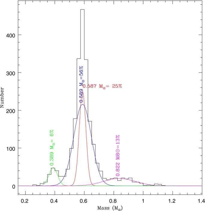
Standard image High-resolution imageThere is no reason to expect the observed mass distribution to be Gaussian. The ingredients are the initial mass function, initial to final mass relation, star formation rate, and mass-loss rates, all of which are more or less well-defined physical non-Gaussian relations. We find it informative, however, to use Gaussian deconvolutions of the mass distributions so we can talk about average/peak masses with some quantifiable meaning attached. We do not claim that each Gaussian component represents a unique contribution to the DA/DB population. Figures 10 and 11 show the DA and DB mass distributions, respectively, broken down into their Gaussian components. Table 3 lists the mass peaks and percentage of objects contained within each. The figures clearly indicate that talking about a mean DA mass is not particularly useful, but a peak mass (seen here at 0.59 M☉) is more useful. The low- and high-mass wings of the DA distributions are not symmetric, nor should they likely be, given the age of the universe ultimately determining the low-mass cutoff for single white dwarf stars. The low-mass DA component, at 0.43 M☉ with 4% of the stars, is probably caused by binary interactions since single star evolutionary models cannot generate these stars in a Hubble time, while the smaller high-mass peak at 0.82 M☉ is likely due to mergers. The peak of the DB mass distribution (Figure 11) at ≈0.6 M☉ is similar that of the DA distribution although the overall shape is quite different.

Figure 10. Histogram of the masses for S/N ⩾ 15 clean DAs hotter than Teff = 13, 000 K and its Gaussian decomposition.
Download figure:
Standard image High-resolution image
Figure 11. Histogram of the masses for S/N ⩾15 clean DBs hotter than Teff = 16, 000 K and its Gaussian decomposition.
Download figure:
Standard image High-resolution imageTable 3. Gaussian Components of Observed DA and DB Mass Distributions
| Component | Mean | Strength |
|---|---|---|
| (M☉) | (%) | |
| DA | ||
| 1 | 0.589 | 56 |
| 2 | 0.587 | 25 |
| 3 | 0.822 | 13 |
| 4 | 0.389 | 6 |
| DB | ||
| 1 | 0.693 | 39 |
| 2 | 0.640 | 35 |
| 3 | 0.599 | 26 |
Download table as: ASCIITypeset image
The Teff distributions shown in Figure 12 do not reveal a DB gap, i.e., we do detect stars with He i-dominated atmospheres hotter than Teff = 30, 000 K, but there does seem to be a decrease of cooler DBs, which simply become DCs, DQs, DZs as they cool below ≈10, 000 K.

Figure 12. Histogram of the Teff distribution for our DA (top) and DB (lower) samples.
Download figure:
Standard image High-resolution image
Although our measured mean mass for our DB sample is higher than that of our DAs, the mass distributions show that the largest number of DBs have masses similar to peak DA distribution. The high-mass tail of the DB distribution could be the result of a varying number of thermal pulses or of varying metallicity in the DB progenitors. It may also be that the higher mass DB progenitors are simply more prone to experience a very late thermal pulse than are lower mass DB progenitors. The trace low-mass component in the DB distribution may be associated with AM CVn stars, double He WDs, and a result of binary evolution.
We thank Matt Burleigh for thorough and useful comments during the referee process. This work was partially supported by the Gemini Observatory which is operated by the Association of Universities for Research in Astronomy, Inc., on behalf of the international Gemini partnership of Argentina, Australia, Brazil, Canada, Chile, the United Kingdom, and the United States of America. Funding for the SDSS and SDSS-II has been provided by the Alfred P. Sloan Foundation, the Participating Institutions, the National Science Foundation, the U.S. Department of Energy, the National Aeronautics and Space Administration, the Japanese Monbukagakusho, the Max Planck Society, and the Higher Education Funding Council for England. The SDSS Web Site is http://www.sdss.org/.
The SDSS is managed by the Astrophysical Research Consortium for the Participating Institutions. The Participating Institutions are the American Museum of Natural History, Astrophysical Institute Potsdam, University of Basel, University of Cambridge, Case Western Reserve University, University of Chicago, Drexel University, Fermilab, the Institute for Advanced Study, the Japan Participation Group, Johns Hopkins University, the Joint Institute for Nuclear Astrophysics, the Kavli Institute for Particle Astrophysics and Cosmology, the Korean Scientist Group, the Chinese Academy of Sciences (LAMOST), Los Alamos National Laboratory, the Max-Planck-Institute for Astronomy (MPIA), the Max-Planck-Institute for Astrophysics (MPA), New Mexico State University, Ohio State University, University of Pittsburgh, University of Portsmouth, Princeton University, the United States Naval Observatory, and the University of Washington. P.D. is a CRAQ postdoctoral fellow. This work was supported in part by NSERC Canada and FQRNT Québec. S.O.K., I.P., V.P., and J.E.S. were supported by FAPERGS and CNPq-Brazil.
Facility: Sloan -
APPENDIX: SQL QUERY LISTINGS
This is the SQL code used to reproduce the Eisenstein et al. (2006a) candidate selection criteria.
SELECT
s.plate, s.mjd, s.fiberid,
p.ObjId, p.psfMag_u, p.psfMag_g, p.psfMag_r, p.psfMag_i, p.psfMag_z,
p.ra, p.dec, s.z, u.propermotion, t.bsz, t.zbclass
FROM SpecObjAll s INNER JOIN PhotoObjAll p ON s.bestObjId=p.ObjID
LEFT OUTER JOIN sppParams t on s.specObjID=t.specObjID
LEFT OUTER JOIN USNO u on s.bestObjID=u.ObjID
WHERE p.psfMag_u <21.5
AND p.extinction_r <=0.6
AND
–either −2 <u−g < 0.833 − 0.667(g−r), −2 < g−r < 0.2
( ((p.psfMag_u-p.psfMag_g between −2 and
(0.833-0.667*(p.psfMag_g-p.psfMag_r)))
and (p.psfMag_g-p.psfMag_r between -2 and 0.2))
OR – or 0.2<g-r<1, |(r-i)-0.363(g-r)|>0.1,
– ( (u-g<0.7) or (u-g<2.5(g-r)-0.5)
((p.psfMag_g-p.psfMag_r between 0.2 and 1)
and (Abs((p.psfMag_r-p.psfMag_i)-0.363*(p.psfMag_g-p.psfMag_r))>0.1)
and ( ((p.psfMag_u-p.psfMag_g)<0.7)
or ((p.psfMag_u-p.psfMag_g)<2.5*(p.psfMag_g-p.psfMag_r)-0.5) )))
AND
—the following is for specBS only; – low redshift and not a galaxy
(((t.bsz <0.003)
and (t.zbclass <> 'GALAXY'))
OR
– flags for all filters are OK
((p.flags_u | p.flags_g | p.flags_r | p.flags_i | p.flags_z) &
(dbo.fPhotoFlags('INTERP_CENTER') |
dbo.fPhotoFlags('COSMIC_RAY') |
dbo.fPhotoFlags('EDGE') |
dbo.fPhotoFlags('SATURATED'))=0)
AND — small measured z with a good z determination
(( (Abs(s.z)<0.003) and
((s.zwarning&1)=0))
OR — large measured z, but with a high proper motion
( (Abs(s.z)>0.003) and
(Abs(u.propermotion)>30) )))
ORDER BY s.plate, s.mjd, s.fiberid
The SQL code below was used to for the second half of candidate generation as discussed in the text.
– find all objects targeted as WD, HOTSTD,
– classified as CV, CWD, WD, WDm,
SELECT t.plate, t.mjd, t.fiberID,
s.targettype, s.seguetargetclass,
s.sptypea, s.zbsubclass,
s.flag,
t.primTarget, t.secTarget, t.seguePrimTarget, t.segueSecTarget
FROM sppParams s left outer join specObjAll t
ON
t.specobjid=s.specobjid
WHERE
— SEGUE TARGETing
(s.targettype LIKE 'SEGUE_WD%') OR
(s.targettype = 'STAR_WHITE_DWARF') OR
(s.targettype = 'HOT_STD') OR
(s.seguetargetclass = 'HOT') OR
(s.seguetargetclass = 'WD') OR
— SEGUE CLASSIFICATIONS
(s.sptypea LIKE '%WD%') OR
(s.sptypea LIKE '%CV%') OR
(s.zbsubclass LIKE '%WD%') OR
(s.zbsubclass LIKE '%CV%') OR
(s.flag LIKE 'D%') —likely WD
(s.flag LIKE 'd%') —likely SD
— TARGETing from SpecObj (primTarget should be same as targettype)
((t.primTarget & 0x000A0000) > 1) OR – WD or CATY_VAR
((t.secTarget & 0x00000200) >1) OR – HOT_STD
((t.seguePrimTarget & 0x000A0000) > 1) OR – WD or CATY_VAR
((t.segueSecTarget & 0x00000200) >1) – HOT_STD
ORDER by t.plate, t.mjd, t.fiberID