


Abstract
The term frustration refers to lattice systems whose ground state cannot simultaneously satisfy all the interactions. Frustration is an important property of correlated electron systems, which stems from the sign of loop products (similar to Wilson products) of interactions on a lattice. It was early recognized that geometric frustration can produce rather exotic physical behaviors, such as macroscopic ground state degeneracy and helimagnetism. The interest in frustrated systems was renewed two decades later in the context of spin glasses and the emergence of magnetic superstructures. In particular, Phil Anderson's proposal of a quantum spin liquid ground state for a two-dimensional lattice S = 1/2 Heisenberg magnet generated a very active line of research that still continues. As a result of these early discoveries and conjectures, the study of frustrated models and materials exploded over the last two decades. Besides the large efforts triggered by the search of quantum spin liquids, it was also recognized that frustration plays a crucial role in a vast spectrum of physical phenomena arising from correlated electron materials. Here we review some of these phenomena with particular emphasis on the stabilization of chiral liquids and non-coplanar magnetic orderings. In particular, we focus on the ubiquitous interplay between magnetic and charge degrees of freedom in frustrated correlated electron systems and on the role of anisotropy. We demonstrate that these basic ingredients lead to exotic phenomena, such as, charge effects in Mott insulators, the stabilization of single magnetic vortices, as well as vortex and skyrmion crystals, and the emergence of different types of chiral liquids. In particular, these orderings appear more naturally in itinerant magnets with the potential of inducing a very large anomalous Hall effect.
Export citation and abstract BibTeX RIS
Corresponding Editor Laura Greene
1. Introduction
Strongly correlated electron systems have captivated several generations of condensed matter physicists because of the vast spectrum of physical phenomena emerging from the competition between the electronic kinetic energy and Coulomb interaction. While the concept of competing interactions embodies the idea of frustration, the latter can be defined in a more rigorous mathematical sense. In general, the competition between kinetic energy and Coulomb repulsion leads to effective interactions with lower characteristic energy scales. These effective interactions can be highly frustrated even for cases in which one bare interaction is dominated by the other one.
As a prototypical example, we will consider the case of Mott insulators deep inside the Mott phase, i.e. with a strong intra-atomic Coulomb repulsion in comparison to the the kinetic energy. The minimal model for describing this class of materials is the Hubbard Hamiltonian,
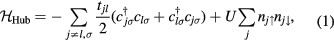
including a tight-binding kinetic energy term with hopping amplitudes tjl and an intra-atomic Coulomb repulsion U. The fermionic operator  annihilates (creates) an electron with spin σ in the atom j. The factor of 1/2 in the first term of
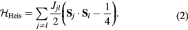
  takes into account the fact that each bond jl is counted twice in the sum. At half-filling (one electron per atomic orbital) and for large enough U/t, the electrons localize around their atomic orbitals because of the large effective barrier produced by the strong Coulomb interaction. The resulting Mott insulator (MI) still contains spin degrees of freedom which are subject to effective interactions arising from a partial electronic delocalization away from their atomic orbitals. To lowest order in t/U, these effective spin–spin interactions are Heisenberg-like and antiferromagnetic (AFM) because of the antisymmetric nature of the fermionic wave-functions (Pauli exclusion principle):
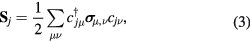
The exchange interactions are  and
and
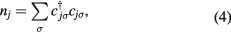
where  is the vector of Pauli matrices.
This Heisenberg Hamiltonian (2) can be frustrated or not depending on the parity of the loops that result from connecting sites of the lattice through their exchange interactions. In the case of  , the system is not frustrated in absence of loops containing an odd number of exchange couplings. This is the case of Hamiltonians defined on bipartite lattices, i.e. lattices that can be subdivided into two sublattices such that the atoms of one sublattice only interact with the atoms of the other sublattice (e.g. square, honeycomb or simple cubic lattices with nearest-neighbor exchange). Loops containing an odd number of AFM exchange interactions are geometrically frustrated, i.e. it is not possible to simultaneously satisfy all the exchange couplings on the loop (see figure 1). In general, when the exchange interactions can be either ferromagnetic (FM) or AFM, we just need to assign a negative (positive) sign to the AFM (FM) interactions. The loop is frustrated if the product of the signs is negative. In particular, the triangular or kagome lattices with nearest-neighbor AFM interactions are simple examples of frustrated systems. In these cases, frustration arises from the triangular nature of the smallest loops and we say that these systems are geometrically frustrated.

Figure 1. Examples of non-frustrated (a) and frustrated (b) loops. As it is explained in section 2, frustrated loops like the triangle shown in panel (b) enable electronic charge effects in Mott insulators. In particular, the spin configuration of panel (b) leads to a net electric dipole  (big arrow).
Download figure:
Standard image High-resolution imageWhile the term 'frustration' was introduced 1977 by Toulouse [1], the earliest work on frustrated magnetism dates back to 1950, when Wannier published his classical work on the AFM triangular Ising model [2]. This seminal work already describes several potential consequences of frustration that make it an attractive area of research. In particular, the macroscopic ground state degeneracy of the AFM triangular Ising model leads to the absence of phase transitions at any finite temperature T: the spin–spin correlation length remains finite for  , implying that the system only exhibits liquid-like correlations down to T = 0. This extensive ground state degeneracy often appears in several highly frustrated models, such as the so called spin-ice systems [3], and it reflects the simple fact that frustration can open the game to a large number of competing phases. Moreover, unlike systems that order at low-enough temperatures, highly frustrated systems can support low-energy excitations with non-trivial topology (like vortices or monopoles) which are ultimately responsible for the finite T liquid-like correlations [4].
From our previous discussion, it is clear that frustration also arises in magnets described by  when the sign of the exchange coupling, Jjl, depends on the relative position,
  , between the two atoms. This is the case of local moment systems, whose exchange interaction is mediated by conduction electrons. The effective exchange coupling is known as Ruderman–Kittel–Kasuya–Yosida (RKKY) interaction [5–7], and it can naturally explain the observation of helical spin arrangements in rare-earth and other itinerant magnets, as it was recognized towards the end of fifties and the beginning of sixties [8–10]. About the same time, the axial (or anisotropic) next-nearest-neighbor Ising (ANNNI) model was introduced by Elliot [10] to describe the modulated phase of erbium [11]. This simple model describes spatially modulated phases whose periodicity changes in a stepwise manner as a function of an external parameter, such as temperature or magnetic field [12, 13]. The periodicity 'locks-in' at a few commensurate values and increasingly refined calculations lead to additional phases, which are stable in extremely narrow temperature intervals consistent with 'a devil's staircase' [13]. The domain-wall or soliton theory for the commensurate-incommensurate transition was developed in this context [14–18].
The study of frustrated materials was reinvigorated in the seventies with the discovery of spin glasses arising from the combination of frustration and disorder [19, 20]. Around the same time, Anderson proposed his resonating valence bond (RVB) state as the ground state of quantum spin liquids [21]. This proposal triggered large efforts for finding realizations of spin liquid ground states in highly-frustrated quantum magnets that still continue nowadays [22]. The large ground state degeneracy of highly frustrated models posed a natural question: can fluctuations of thermal or quantum origin split this degeneracy? The answer to this question led to the concept of 'order by disorder', which was introduced by Villain and co-workers in 1980 after considering a frustrated Ising model on a square lattice [23].
Over the last three decades, we have witnessed an explosion of work on frustrated models and materials. The above-mentioned behaviors enabled by frustration were observed and further studied in multiple compounds. Moreover, some notions, like the concept of quantum spin liquid, were further elaborated and investigated. New developments in real space visualization techniques unveiled even more complex superstructures emerging from frustration. Indeed, it was recently recognized that the one-dimensional superstructures observed and explained in the sixties can be superseded by multiple- orderings (
 is the ordering wave-vector), i.e. magnetic orderings that are modulated along different directions. These orderings include vortex and skyrmion crystals emerging from the competition between two or more exchange interactions in high-symmetry environments.
The purpose of this article is to review some exotic states of matter and response functions enabled by frustration, which were mainly studied over the last decade. The diversity of these novel phenomena suggests that frustrated materials are still full of surprises, making frustration a useful guiding principle in the search for novel emergent behaviors. In section 2 we demonstrate that geometric frustration is a precondition for having non-trivial charge effects in MIs: the effective charge and electric current density operators are non-zero only if the system is frustrated. In particular, we derive the effective charge and current density operators for a single band Hubbard model in the large U/t limit. In section 3 we propose different scenarios for the stabilization of non-coplanar (chiral) magnetic textures in Mott systems. In particular, we demonstrate that impurities, such as a non-magnetic ion, can bind magnetic vortices above the saturation field of a large class of frustrated magnets. Moreover, we show that a periodic array of non-magnetic impurities (charge density wave of holes) induces a rich thermodynamic phase diagram as a function of temperature and magnetic field, which includes a high field 3Q-vortex crystal phase, among other chiral orderings. For clean systems, we show that the combination of geometric frustration and easy-axis anisotropy leads to magnetic field induced spontaneous skyrmion crystals. Section 4 describes the effects of frustration on the stabilization of non-coplanar magnetic orderings and chiral liquids in itinerant magnets. We use a Kondo lattice model with classical local moments to describe the basic concepts that produce the stabilization of multiple- orderings in itinerant systems. In particular, we show that some of these orderings can produce a very large anomalous Hall effect or even quantum anomalous Hall effect. The final conclusions appear in section 5.
2. Charge effects in Mott insulators
The new century started with a renewed interest in magneto-electric effects. It was noticed that even weak magnetoelectric interactions can lead to spectacular cross-coupling effects in MIs when electric polarization is induced by magnetic ordering [24]. Most efforts for understanding the microscopic mechanisms behind giant magneto-electric effects focused on the ionic displacements induced by certain magnetic orderings [25–29]. However, it was later recognized that purely electronic charge effects also exist in MIs [30]. Indeed, the possibility of having a spontaneous electronic polarization in correlated insulators had been already pointed out in the context of the ionic Hubbard model and of an extended Falicov–Kimball model [31–34].
Interestingly enough, frustration is a precondition for the existence of non-trivial electronic charge effects in MIs. As we already mentioned, the Hubbard model (1) is the minimal Hamiltonian for describing the physics of MIs. The charge density operator,
and the current density operator,
with  are related by a continuity equation on the lattice,
  = 0, arising from charge conservation:
 ![$[{{\mathcal{H}}_{\text{Hubb}}},\sum\nolimits_{j}{{n}_{j}}]=0$](https://content.cld.iop.org/journals/0034-4885/79/8/084504/revision1/ropaa280aieqn015.gif) . It is important to note that the kinetic energy term of
. It is important to note that the kinetic energy term of  ,
,  , changes sign under the charge conjugation transformation:

In other words, the hopping amplitudes tjl change sign under charge conjugation. Naturally, both the deviation of the charge density (4) from the half-filling and the current density (5) operators also change sign under this transformation. The current density operator on the bond jl is proportional to tjl, so the change of sign of this operator arises from the change of sign of tjl because  remains invariant. In addition, the spin operators (3) remain unchanged under charge conjugation:
This is indeed the expected property given that charge conjugation simply changes the sign of the charges, while it leaves the time direction unchanged (velocities do not change under this transformation).
As we already explained, at half-filling and for large enough U/t, the low-energy sector of  contains states with roughly one electron in each atom. In particular,
  has 2N degenerate ground states for tjk = 0 (N is the total number of atoms in the lattice) because the spin of each electron can either be up or down. States in this unperturbed ground space will be denoted by
  . The massive degeneracy is lifted for finite
  and the new low-energy eigenstates,
  , can be obtained by applying a unitary transformation to the states
  :
:  .
.  is the (antihermitian) generator of the unitary transformation. The effective low-energy operator
  for a given observable
  is obtained by projecting it into the low-energy subspace spanned by the states
  . However, in order to express
  as a function of spin operators only, it is necessary to work in the basis of
  states. In this basis we have
  where
where  is the projector on the subspace generated by the states
  , while
  projects on the subspace generated by the the singly-occupied states
  . For
. For  we obtain the effective AFM Heisenberg spin Hamiltonian given in equation (2) by expanding
  up to first order in tjl/U.
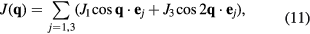
In a similar way, we can obtain the effective operators for the charge and electric current density operators (4) and (5) (see appendix). As these operators are odd under charge conjugation, nonzero perturbative terms arise only at odd orders in tjl. Then, because the smallest loop in a lattice is a triangle, contributions to the effective current density operator must involve at least three spins. Given that the electric current density is a scalar under spin rotations and odd under time reversal, the three spin (jkl) contribution must be proportional to the scalar spin chirality  [30]:
[30]:
where  , and the summation over l corresponds to different three-spin paths containing the bond jk. An immediate consequence of equation (8) is that scalar chiral ordering is a precondition for having loop electric currents in Mott insulators. The scalar spin chiral ordering
  can exist even in absence of magnetic ordering [35–37]. These phases are usually called 'chiral liquids' and equation (8) provides a natural observable (orbital magnetic moments) for detecting them.
The charge density operator nj is a scalar under spin rotations and even under time reversal, implying that three-spin contributions (jkl) must consist of a linear combination of scalar products of two spin operators [30]:
with  . The sum of the prefactors in front of each of the three scalar products must be equal to zero because of the Pauli exclusion principle:
  must be exactly equal to one on a triangle of three fully polarized spins (
 to all orders in perturbation theory). If we evaluate equation (9) for the spin configuration of the triangle shown in figure 1(b), we can easily verify that for positive tij amplitudes there is an electronic charge displacement from the site j with the unpaired spin to the sites i and j that form the FM bond. As it is shown in the figure, this charge displacement leads to an electric dipole pointing in the opposite direction because the electron charge is negative.
In general, equation (9) predicts that orderings which break the equivalence between bonds, known as bond-orderings, will induce an electronic charge density wave. In particular, this phenomenon can lead to multiferroic behavior and giant magneto-electric effects when the charge density wave has a net electric polarization [38]. Equation (9) has been recently extended to include the effects of finite relativistic spin–orbit coupling [39, 40].
As we mentioned, both the charge and current density operators can only contain odd contributions in the hopping amplitudes because both operators are odd under charge conjugation. In addition, perturbative contributions to any effective operator must always connect states in the low-energy subspace generated by the singly-occupied states  . These processes arise from loops (including retraceable paths), like the ones shown in figure 2. In particular, as it is shown in the same figure, a Hubbard model on a bipartite lattice can only generate contributions which are even in the hopping amplitudes. This simple observation implies that the effective charge and current density operators are identically zero on unfrustrated systems. Non-zero contributions can only arise from loops closed by an odd number of hopping terms, i.e. from frustrated loops.

Figure 2. Example of a bipartite (square) lattice. An even number of hopping processes is needed to close any arbitrary loop.
Download figure:
Standard image High-resolution imageIt is interesting to note that frustration also plays an important role in the charge effects of MI's induced by spin-lattice coupling. The ionic-based mechanisms rely either on the magnetostriction induced by certain bond orderings (both the bond angle and the bond length are modulated by a periodic change in the scalar product of two neighboring spin moments  ) or on the spin–orbit interaction, which triggers an ionic displacement for spiral spin orderings. Spiral spin orderings are characterized by a non-zero vector chirality
  between neighboring spins. The so-called 'inverse Dzyaloshinskii–Moriya (DM)' mechanism produces a net electric dipole proportional to
  (
( is the relative unit vector between the spins j and l) [25–27]. The polarization is induced by the displacement
  of a third ion (with charge qI) away from the bond center (this ion mediates the super-exchange interaction between spins i and j). The induced DM interaction,
  , lowers the magnetic energy by an amount
  , which is linear in
  . Because the elastic energy cost is quadratic in
  , the electric polarization
  is finite as long as
  . In both cases, frustration provides a natural mechanism for stabilizing the bond or spiral orderings required by these ionic-based mechanisms.
Finally, it is interesting to compare the strength of the ionic and the electronic contributions to the electric dipole moments that can appear in MIs. As we have seen in this section, the electronic contribution is of order  in the small t/U limit, where a is the lattice constant. On the other hand, the ionic displacement due to magnetostriction is of order
  , where
  is the derivative of the exchange constant J as function of the distance r between the two magnetic ions and K is the elastic constant for the lattice distortion. Given that this ionic displacement is normally a very small fraction of the lattice parameter,
  10−4, we note that the electronic contribution can easily dominate over the ionic contribution. In particular, the electronic dipole can become a sizable fraction of ea (e is the electron charge) if the MI is not far from the Mott transition.
3. Non-coplanar textures of frustrated Mott insulators
3.1. Magnetic vortex induced by impurity
As we have seen in the previous section, certain spin orderings lead to non-trivial charge effects in Mott Insulators. In particular, orbital currents arise from nonzero scalar spin chirality:  . While chiral ordering can exist even in absence of magnetic ordering (
 ), it is clear that non-coplanar magnetic (
 ) orderings have a non-zero local chirality
  . The purpose of this section is to show how non-coplanar magnetic orderings can emerge from frustration in local moment systems. We will then consider the simple example of a triangular spin S Heisenberg model with a FM nearest-neighbor exchange, J1 < 0, and an AFM third-nearest-neighbor exchange J3:
The first sum runs over nearest-neighbor bonds  , while the second sum runs over third-nearest-neighbor bonds
  . From now on, we will use the lattice parameter, a, as our length unit.
The relative position vectors of the nearest-neighbors of a given atom in the triangular lattice are  (
( ), with
  ,
,  and
and  . For what follows, the main role of the competing real space interactions, J1 and J3, is to induce an exchange interaction in momentum space,
with a local maximum at  and global minima at six wave-vectors
  (
( ) connected by the C6 symmetry group of the triangular lattice. The magnitude of these vectors is:
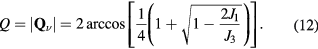
According to equation (12), the system is a ferromagnet (Q = 0), for  . The ordering wave-vector becomes nonzero for
  . Therefore,
  is the Lifshitz transition point from FM (Q = 0) to incommensurate (
 ) AFM ordering. Correspondingly, the saturation field (magnetic field required to fully saturate the magnetic moments) also becomes finite for
  :
:

Clearly,  for
for  because
 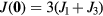 . Right above
  , we can expand in the small parameter
  :
:

In addition, we can expand equation (12) to obtain:
which implies that Hsat is proportional to Q4 near the Lifshitz point  .
.
We will assume now that  and that the magnetic field H is larger than Hsat. We want to know the effect of replacing one spin by a non-magnetic impurity. It has been shown recently that non-magnetic impurities lead to non-coplanar spin structures in the triangular Heisenberg model with a nearest-neighbor AFM interaction [41–43]. In contrast, here we will consider the effect of non-magnetic impurities on frustrated magnets with competing FM and AFM interactions. Given the FM nature of J1, the saturation field of the spins near the impurity must be higher than the saturation field Hsat far away from the impurity. This simple observation implies that the spins should cant away from the z-axis around the non-magnetic impurity.
The spin texture far away from the non-magnetic impurity can be obtained by taking the continuum limit  . In this limit,
  becomes

with
up to sixth order in a gradient expansion and  . Given that the leading order amplitude of the C6 anisotropy is Q6, we can neglect
  for
for  . In addition, we will rescale our energy, length and magnetic field units in order to normalize the coefficients [44]
In the new units the saturation field is  and
and  . Equation (19) is the universal theory for centrosymmetric frustrated magnets near a Lifshitz point.
To model the effect of the non-magnetic impurity located at the origin, we simply need to modify the stiffness  near the origin. We note that
  is enhanced near the origin because of the suppression of J1 on the bonds connecting the non-magnetic impurity and its nearest neighbors. Therefore, we will replace the spatially uniform δ with

where  is the Heaviside step function, r0 is the range over which the local stiffness is modified by the presence of the impurity, and
  is a positive dimensionless parameter. We note that a similar continuum model is valid for other types of impurities. The choice of the step function is arbitrary because details of this non-universal function do not affect the asymptotic behavior of the solution for
  .
.
As we explained above, the saturation field near the impurity,  , is bigger than the bulk saturation field
  . The nature of the magnetic distortion around the impurity is obtained from the structure of the lowest energy internal mode (localized mode around the impurity), which becomes gapless at
  . We will then compute the normal modes of the fully polarized phase in order to determine this instability. To describe the small oscillations around the ground state configuration, we introduce the bosonic field
  via the Holstein-Primakoff transformation
By expanding  up to quadratic order in
  , we obtain the spin-wave Hamiltonian density:

The resulting equation of motion for  is:
is:

In absence of the impurity (translationally invariant case), the eigenmodes are magnons with a dispersion relation,
obtained by Fourier transforming the equation of motion equation (23). This expression shows explicitly that  , i.e. the magnon gap is
  . We note that the magnetic field enters as an additive constant that shifts the whole spectrum. This is so because it couples to the conserved quantity
  (total magnetization along the z-axis).
In the presence of the impurity, we need to replace the spatially uniform stiffness  by the non-uniform stiffness,
  , given by equation (20). The eigenmodes,
  , are now created by operators of the form
  , where
  is an eigenfunction of the operator
  . While translational symmetry is broken by the presence of the impurity, rotational symmetry is still preserved. Consequently, it is useful to introduce polar coordinates
  and work in the basis of eigenstates of
  with well defined angular momentum l. These circular waves are described by the Bessel functions of the first kind:

For  , the stiffness is constant and equal to
  . Therefore, the eigenmodes in this region are linear combinations of two circular waves

with the two momenta,  , that produce the same energy eigenvalue ω:
Because we are looking for bound states, the corresponding eigenmodes must decay exponentially for  . Therefore, we need to use the modified Bessel functions of the second kind for r > r0, which are also eigenvectors of the Laplacian operator:

Once again, the eigenvector for r > r0 is a linear combination of two of these functions

with momenta  that produce the energy eigenvalue ω and lead to an exponential decay for
  :
:
We note that  because we are looking for bound states, which must lie below the magnon gap
  . The last part of the calculation is to ask that the eigenmodes and their three first derivatives must be continuous at r = r0. This condition arises from the fourth order nature of the differential equation (23).
At this point, it is clear that the problem under consideration is analogous to the quantum mechanical problem of a single particle moving in 2D with an effective mass that depends on its distance to the origin (it takes one value for r > r0 and a different value for  ). However, an important difference relative to the usual single-particle problem is that the energy minimum occurs at a finite wave-vector k = Q (see equation (24)):
  is flat on the circle for radius k = Q and it has a finite dispersion along the radial direction. This implies that the density of single magnon states,
  , has the same singularity as a one-dimensional (1D) system when ω approaches the bottom of the single magnon dispersion
  :
:  for
for  . As it is well known, this singular behavior of
  leads to the formation of a bound state for an infinitesimal attractive potential well. In particular, the 1D-like divergence in
  produces a binding energy,
  , which is proportional to the square of the amplitude of the attractive interaction,
  , in contrast to the essential singularity that appears for the usual 2D problem with a single minimum at k = 0.
In the case under consideration, the effective attraction is produced by an increase in the absolute value of the stiffness for r < r0, which is felt by all the circular waves regardless of their angular momenta l. Given that the density of states exhibits the same singularity for any value of l, we expect the formation of a bound state for each value of l. The l-value of the lowest energy bound state determines the nature of the magnetic distortion around the impurity right below  .
.
For weak attraction,  , the amplitude of the attractive interaction in the l channel is
Given the asymptotic form of the Bessel functions for small argument,  for
for  , gl is maximized for l = 0 if
  . However, it is easy to verify that this is not necessarily true when r0 Q becomes bigger than one (see inset of figure 3). In particular, gl acquires its maximum value for
  when r0Q becomes of the order or bigger than the first root of J1(z), as it is shown in figure 3. Moreover, a generalized impurity that increases
  in the ring
  will maximize gl for
  -values, which increase monotonically with R. This type of impurity corresponds to removing spins from a ring of sites, instead of the single-site (R = r0/2) that we are currently considering [45].

Figure 3. Effective bare attractive interaction  in the weak-coupling regime as a function of the range r0 of the impurity potential for different values of the angular momentum l = 0, 1, 2. The inset shows the corresponding Bessel functions that appear in the expression (31).
Download figure:
Standard image High-resolution imageFigure 4 shows the bound state energies  of the l = 0, 1, 2 channels as a function of
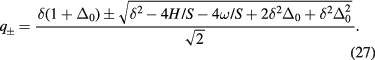
  for r0 = 2 and for r0 = 4. Interestingly enough, the l = 1 bound state becomes the ground state above a critical value of the impurity potential
  for r0 = 2, while it is already the ground state for arbitrarily small values of
  if r0 = 4. This result implies that the leading instability around an impurity in a frustrated magnet can be a magnetic vortex with winding number
  . Moreover, strong impurity potentials (larger values of
  ) can produce lowest energy bound states with even higher values of l, i.e. vortices with winding numbers larger than on will emerge below
  .
.

Figure 4. Binding energies  for l = 0, 1, 2 as a function of
  for (a) r0 = 4 and (b) r0 = 2. The insets of each panel show the energy difference between the energies of the l = 1, 2 and the l = 0 bound states. For r0 = 4, the ground state alternates between the l = 0 and l = 1 bound states as a function of increasing
  . For r0 = 2, the l = 1 bound state becomes the ground state above a critical value of
  .
.
Download figure:
Standard image High-resolution imageThe main conclusion of our semi-classical stability analysis is that impurities can nucleate magnetic vortices in frustrated magnets well above the bulk saturation field. This conclusion can be explicitly verified in the classical limit. To find the actual distortion induced by the non-magnetic impurity below  , we solve numerically the Landau–Lifshitz–Gilbert equation of motion for the classical limit of
  :
:

Here α is the Gilbert damping and  is the effective magnetic field acting on each spin. The non-magnetic impurity is introduced by setting the spin at the origin to 0:
  . Consistently with our previous analysis, a vortex is nucleated around the impurity once the system is allowed to relax from an initial fully polarized state.
As it is shown in figure 5, the linear vortex size increases upon approaching the bulk saturation field  . Indeed, by solving the Euler-Lagrange equations of the continuum model for
  , one can verify that the vortex amplitude (tilting of the spins away from the z-axis) decays exponentially over the magnetic correlation length ξ, which diverges as
  upon approaching the bulk saturation field Hsat. In other words, the vortex radius diverges at the critical point
  , where the exponential decay is replaced by an algebraic decay
  [45]. This algebraic decay signals a second order transition into a conical single-
 magnetic ordering that will be considered in the next sections.

Figure 5. Magnetic vortex bound to a non-magnetic impurity for different values of the magnetic field above the bulk saturation field  .
.
Download figure:
Standard image High-resolution imageFinally, we note that a similar calculation can be easily extended to quantum spin systems of arbitrary spin S. In this case, the modes for  are obtained by diagonalizing the quantum version of
  in the
  sector, i.e. in the subspace of states with a single-spin flip (
 ) relative to the fully polarized ground state. As it is illustrated in figure 6, the flipped spin can be regarded as a single particle moving in the central potential generated by the impurity at the origin. If we assume that the impurity consists of a smaller magnetic moment
  (the non-magnetic impurity corresponds to
  ), the flipped spin has a lower energy,
  (J1 < 0) when sitting on the first hexagon of nearest-neighbor sites around the impurity (potential well) and a higher energy
  (potential barrier) when sitting on the six third-nearest neighbors (see figure 6). The hopping amplitude between a pair of sites j and l away from the origin is Jjl S. The hopping amplitude between the impurity site and a different site l is
  . It is then clear that the total spin S is an overall scaling factor for the effective single-particle Hamiltonian. In other words, the normal modes depend only on the ratio
  , implying that for the case of a non-magnetic impurity (
 ) the normal modes are exactly the same all the way from the S = 1/2 quantum limit to the
  classical limit. This fact remains true for any finite
  as long as we keep the
  ratio fixed while varying S, and it explains why the equation of the motion for the eigenmodes in the classical spin limit (23) is formally the same as the single particle Schrödinger equation.

Figure 6. An impurity of spin  (central blue circle) is located at the origin of the triangular lattice with nearest neighbor FM exchange J1 and third nearest neighbor AFM exchange J3. All the spins are fully polarized along the z-direction except for one (crossed circle) that has been flipped to the Sz = S − 1 state. This flipped spin propagates like a particle with effective nearest-neighbor hopping J1 S and third-nearest-neighbor hopping J3. The impurity modifies these hopping amplitudes (
 ) and it changes the diagonal energies of the six nearest-neighbor sites denoted by a red hexagon
  and on the six third-nearest-neighbor sites denoted by open blue circles
  .
.
Download figure:
Standard image High-resolution imageAs expected from our previous analysis, the ground state for the single spin-flip subspace of the quantum  Hamiltonian with a non-magnetic impurity (
 ) corresponds to two degenerate bound states with quasi-angular momentum
  (the phase of the bound state wave function has a winding number
  ) (see figure 7). As we explained before, this bound is the precursor of the vortex state that appears around the impurity below the magnetic field,
  , at which the energy of the bound state becomes equal to the energy of the fully polarized state:
  . The absolute value of the binding energy,
  , reaches its maximum value near
  and it decreases for larger values of
  when the system approaches the other incommensurate to commensurate transition for
  . This is indeed the expected behavior given that the potential well disappears for
  (
( ) and only the potential barrier (
 ) remains.

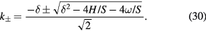
Figure 7. Binding energy of  bound state around the impurity for the quantum version of
  . A single spin-flip relative to the fully polarized state propagates like a single-particle and feels the impurity potential depicted in figure 6. The absolute value of the binding energy,
  , is equal to the difference between the saturation field around the impurity,
  , and the bulk saturation field
  . The inset shows the ratio
  as a function of
  .
.
Download figure:
Standard image High-resolution imageThe inset of figure 7 shows the ratio  as a function of
  . The window of magnetic field values where the non-magnetic impurity is expected to bind a vortex is a sizable fraction of the bulk saturation field, Hsat, for
  . While we have used a particular Hamiltonian,
  , for describing the creation of magnetic vortices by non-magnetic impurities above the bulk saturation field, our conclusion is valid for a larger set of frustrated Hamiltonians, which exhibit a Lifshitz transition from a commensurate FM state to incommensurate helical ordering. The FM interaction, represented by J1 in our model, is necessary to have
  , i.e. to have a bound state around the impurity. The underlying lattice does not need to have C6 symmetry. Vortex sates around non-magnetic impurities should also exist on tetragonal systems (C4 symmetry) [45].
NiGa2S4 provides an experimental realization of  with a ratio
  [46]. Unfortunately this small ratio leads to an extremely narrow magnetic field window above Hsat for observing the vortex-impurity bound state. NiBr2 is an alternative realization of
  with
with  [47]. The saturation field is very high (
 KOe) in this compound because of the presence of a rather strong inter-layer AFM exchange. Non-magnetic impurities can by introduced in this compound by replacing Ni with Zn [48]. Based on the results presented in this section, we predict that ZnxNi1−xBr2 should exhibit magnetic vortices bounded to the Zn-impurities right above the saturation field. Moreover, these vortices should persist below the saturation field [45]. This observation could explain the results of neutron diffraction experiments on a single-crystal of ZnxNi1−xBr2 containing 8-mole% of Zn2+ , which show that the helical propagation wave-vector direction becomes 'disordered', i.e. the incommensurate peaks of the magnetic structure factor form a regular hexagonal structure around the commensurate wave vector [48].
CeRhAl4Si2 and CeIrAl4Si are examples of tetragonal frustrated magnets with competing FM and AFM interactions, which exhibit incommensurate intra-layer magnetic ordering at zero field and low enough temperature [49, 50]. Given that these compounds are easy-axis antiferromagnets, magnetic vortices around non-magnetic impurities should be observed above the meta-magnetic transition induced by a magnetic field parallel to the c-axis. We also note that the metallic character of these materials, whose local moments are provided by localized f-electrons that interact with each other via the RKKY interaction, does not modify our previous analysis. The theory presented in this section applies both to MI's and to itinerant magnets.
It is important to mention that the nearest-neighbor FM exchange also leads to the formation of two magnon bound states above Hsat [51–53]. This implies that for finite spin S, the bulk saturation field is in general higher than the value associated with a single-magnon condensation (see equation (13)). The attractive magnon–magnon interaction can lead to a continuous transition into some multipolar ordering (e.g. nematic ordering for the condensation of magnon pairs) [54–59] or to a discontinuous transition. In any case, the important observation is that the magnitude of the magnon–magnon interaction is of order one, while the attractive interaction,  , between the magnon and a non-magnetic impurity is proportional to S, implying that
  remains higher than Hsat for large enough S. Another factor that makes the magnon-impurity binding energy larger than the magnon–magnon binding energy is the static nature of the impurity: the reduced mass for the two-magnon problem is half of the single magnon mass relevant for the magnon-impurity bound state formation.
Finally, it is worth mentioning that impurities can also nucleate vortices above the saturation field of frustrated magnets with two or more competing AFM interactions, as long as the saturation field near the impurity remains higher than the bulk saturation field. This condition requires that the impurity must distort the lattice locally in order to enhance the the AFM exchange interactions on the neighboring bonds.
3.2. Vortex and skyrmion lattices
3.2.1. Periodic array of impurities.
In the previous section we found that a magnetic vortex forms around a single impurity in a finite interval of magnetic field above the saturation field. We will consider now the effect of a periodic array of impurities. This situation can be realized in a doped system with a finite concentration of holes if the inter-hole Coulomb interaction induces strong charge ordering, i.e. the holes become strongly localized in a periodic structure. This situation has been observed in some high-Tc and related materials for a hole concentration x = 1/8, [60, 61] although the Heisenberg term of the t − J model that describes these materials is not frustrated [62]. The question that we will address now is: what is the effect of a charge-density-wave (CDW) ordering on the magnetic structure in frustrated systems? While the answer to this question will of course depend on the nature and period of the CDW structure, our only purpose here is to show that spontaneous chiral magnetic orderings emerge quite naturally out of the interplay with the underlying charge ordering.
To simplify the discussion we will consider the simple case of a periodic array of non-magnetic sites (holes) forming a triangular superlattice structure with primitive reciprocal lattice vectors  and
and  . To avoid frustration between the magnetic and the charge ordering, we will choose
  and
and  to be commensurate with the magnetic ordering wave vectors
  . In particular, we will set
  (for which
  ) and we assume a CDW with
  , which, as depicted in the inset of figure 8(b), corresponds to a triangular superlattice with the lattice spacing eight times larger than the original lattice parameter. We note also that
  holds in this case.
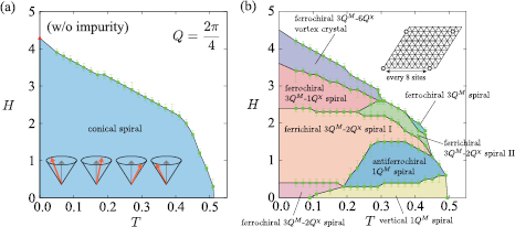
Figure 8. T-H phase diagrams for (a) spatially uniform case and (b) periodically-distributed non-magnetic impurities with primitive reciprocal lattice vectors 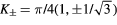 . The values of the exchange interactions are
  and J3 = 1.0 (
 ). The periodicity of non-magnetic impurities is shown in the inset of panel (b).
Download figure:
Standard image High-resolution imageWe extend the  Hamiltonian (equation (10)) to include the nonmagnetic impurities with the prescription,
where pj = 0 (1) corresponds to the presence (absence) of a quenched hole or non-magnetic impurity at the site i. Figure 8 shows the thermodynamic phase diagrams obtained from Monte Carlo (MC) simulations in the absence (figure 8(a)) and the presence of the CDW (figure 8(b)). The different phases of these phase diagrams are characterized by the spin structure factor,
and the chirality structure factor, which we define for both the up and the down triangles ( , respectively) as
where  run over sites of the specified (
 ) sublattice of the dual honeycomb lattice.
  is the spin scalar chirality associated with a triangle centered at
  given by

where j, k, and l are the sites aligned counterclockwise on this triangle. We also introduce the following notations for the total scalar chirality from the upward ( ) and the downward (
 ) triangles and their sum:
The phase diagram in absence of the CDW is rather simple (see figure 8(a)), including only the single- conical spiral phase in addition to the paramagnetic state. In this phase, the xy spin components are quasi-long-range ordered in a magnetic field and they develop long range order (LRO) only at T = 0. However, the C6 symmetry is broken at finite T and H because of the antisymmetric bond ordering characterized by the bond parameter
  (note that this order parameter breaks only discrete symmetries).
The phase diagram becomes much more complex in the presence of the CDW (figure 8(b)). The main qualitative difference relative to the single- conical spiral phase obtained in absence of the CDW is the emergence of a net chiral component,
  , in most of the new phases. Exceptions to this rule are the vertical 1QM spiral ordering and the antiferrochiral 1QM spiral phases that appear next to the paramagnetic phase in the low field region. These are also the only two phases that exhibit single-
 magnetic ordering. Notably, many phases support long-wavelength modulation of local scalar chirality (chirality wave), which is not necessarily single-
 (hereafter, our convention is to use QM and
  , respectively, when it is necessary to make an unambiguous distinction between spin and chirality textures). The stability of each phase in thermodynamic limit is confirmed by performing a finite-size scaling analysis presented in [63].
Figure 9 shows a sequence of snapshots of the spin configurations of the low-temperature phases from zero (figure 9(a)) to the saturation field (figure 9(j)). We also show the square root of the corresponding xy ( ) and z (
 ) components of the spin structure factor in equation (34), where
  . Similarly, figure 10 includes snapshots of the real-space chirality distribution of each phase, along with the square root of chirality structure factors,
  and
and  , for the up and down triangles of the triangular lattice which are the two sublattices of the dual honeycomb lattice), respectively.

Figure 9. Snapshots of spin configurations and the corresponding structure factors (after averaging over 500 MC steps to remove short wavelength fluctuations) for the low temperature phases in the phase diagram of figure 8(b). The second and third columns include the square root of the spin structure factors,  and
and  , to emphasize the secondary
  -components. The field-induced
  component has been subtracted to highlight the Bragg peaks induced by spontaneous symmetry breaking. The first line of panels ((a)–(c)) corresponds to the low field ferrochiral 3QM-
 spiral phase. The second line ((d))–(f)) corresponds to the ferrichiral 3QM-
 spiral I phase. The third, ((g))–(i)), and fourth, ((j)–(l)), lines correspond to the ferrochiral 3QM-
 spiral and the ferrochiral 3QM-
 vortex crystal, respectively. The circles with solid (dashed) lines indicate the dominant (subdominant) peak(s) except for
  .
.
Download figure:
Standard image High-resolution image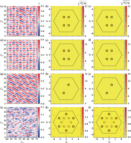
Figure 10. Snapshots of chirality configurations and the corresponding chirality structure factors (after averaging over 500 MC steps to remove short wavelength fluctuations) for the low-T phases in the phase diagram of figure 8(b). The second and third columns include the square root of the chirality structure factors,  and
and  , to emphasize the secondary
  -components. The field-induced
  component has been subtracted to highlight the Bragg peaks induced by spontaneous symmetry breaking. The first line of panels ((a)–(c)) corresponds to the low-field ferrochiral 3QM-
 spiral phase. The second line ((d)–(f)) corresponds to the ferrichiral 3QM-
 spiral I phase. The third, ((g)–(i)), and fourth, ((j)–(l)), lines correspond to the ferrochiral 3QM-
 spiral and the ferrochiral 3QM-
 vortex crystal, respectively. The circles with solid (dashed) lines indicate the dominant (subdominant) peak(s) except for
  .
.
Download figure:
Standard image High-resolution imageAt very low fields, the magnetic ordering consists of a double- chiral phase with a net chiral component (ferrochiral 3QM-2
 spiral). The net chirality has the same sign on the two sublattices of up and down triangles,
  , which is therefore denoted as ferrochiral. The non-zero chirality does not seem to be consistent with the spin configuration shown in figure 9(a), which looks similar to a vertical 1QM spiral ordering with the spiraling moments in the vertical plane. However, upon looking at the spin structure factors shown in figures 9(b) and (c), it becomes clear that this spin ordering contains additional
  components, which render the spin configuration non-coplanar. This is due to the commensurate relation between
  and
and  . For example,
  and
and  are connected by
  , which means that periodic impurities favor multiple- Q orderings and can extend their stability to the H = 0 axis.
Upon increasing the magnetic field, the ferrochiral 3QM-2 spiral phase is replaced by a ferrichiral 3QM-2
 spiral ordering. By ferrichiral, we mean that the scalar spin chirality has different magnitude for up and down triangles, i.e.
  , as it is shown in figures 10(e) and (f). The other difference relative to the zero field phase is that
  has two dominant
  components with the same intensity and a weaker third component, as it is shown in figure 9(f). This explains the anisotropic three-
 modulation that is observed in the real space spin configuration shown in figure 9(d). Interestingly enough, upon increasing temperature this phase transitions into a different ferrichiral 3QM-2
 spiral phase (denoted as ferrichiral 3QM-2
 spiral II in figure 8(b)) that exhibits different intensities for the two dominant
  -components of the chirality distribution. A third phase, denoted as ' ferrochiral 3QM vortex crystal' ordering in figure 8(b), appears upon further increasing the temperature. This phase is characterized by a net,
  , component of the scalar spin chirality,
  .
.
The new phase that appears upon further increasing the magnetic field at low temperatures exhibits a single- modulation of the scalar chirality, as it is clear from the stripy chirality pattern shown in figure 10(g) and denoted as ferrochiral 3QM-
 spiral. The red/blue stripes correspond to opposite signs of the scalar chirality. A net scalar chirality arises from the fact that the holes occupy sites inside the stripes of a given sign. The suppression of the scalar chirality in their proximity leads to a net chirality of the opposite sign.
Finally, the last phase before the system becomes fully saturated is a ferrochiral 3QM-6 vortex crystal similar to the one reported recently for frustrated quantum magnets [64, 65]. As is it shown in figure 10(j), vortices with the same winding number (±1) or vorticity form a triangular lattice. The lattice of holes is one of the three sublattices of the vortex triangular crystal. Like in the case of [64], vortices with opposite winding number (antivortices) appear at the boundary between two vortices and produce the opposite sign of the scalar spin chirality. This is the blue region in figure 10(j) that appears around the red chiral spots arising from the triangular vortex crystal. As it is clear from the spin and chirality structure factors, the six-fold rotational symmetry of the underlying CDW is restored in this phase. The main difference relative to the high-temperature ferrochiral 3QM vortex crystal phase is that six peaks of the chirality structure factor at
  in the ferrochiral 3QM-6
 vortex crystal exhibit long range ordering. Once again, the ferrochiral 3QM-6
 vortex crystal has a net scalar spin chirality because one third of the vortices with a given vorticity (sign of the scalar chirality) have a hole at the center of their cores. These holes suppress the scalar chirality of these vortices (see figure 10(j)) producing an unbalance relative to the contribution of the antivortices.
The corollary of the last two sections is that non-coplanar chiral structures can easily arise from the combination of geometric frustration and inhomogeneous structures. In particular, we have seen that a non-magnetic impurity nucleates a magnetic vortex around it and that a periodic array of non-magnetic 'impurities' (CDW) that is commensurate with the magnetic ordering wave-vectors leads to a rich field- temperature phase diagram with different chiral phases. In particular, as expected from the solution of the single non-magnetic impurity above the bulk saturation field, the highest field broken symmetry state corresponds to a ferrochiral 3QM-6 vortex crystal.
3.2.2. Easy-axis anisotropy and skyrmion crystals.
We have shown in the previous sections that a single impurity can induce a magnetic vortex and that periodic arrays of impurities can stabilize a magnetic vortex crystal. For the triangular lattice under consideration, the vortex crystal corresponds to one type of non-coplanar 3- magnetic ordering. It is then natural to ask if non-coplanar 3-
 orderings can also be stabilized in absence of impurities or density-waves of a different order parameter that render the medium inhomogeneous.
In general, non-coplanar magnetic orderings are quite scarce among isotropic Mott insulators. In principle, they can appear as multiple- orderings whenever the Fourier transform of the exchange interaction,
  , has global minima at multiple symmetry related wave-vectors
  . The basic difficulty is that, unlike the case of single-
 magnetic ordering, the magnitude of the moment is in general modulated for the multiple-
 orderings. (This is not necessarily true when
  are high-symmetry wave-vectors). This modulation is penalized by the longitudinal stiffness of the magnetic moments, which becomes infinitely large in the
  and
and  limit. In other words, the length of the magnetic moments is fixed in this limit, implying that the multiple-
 orderings must contain higher harmonics, which necessarily increase the exchange interaction energy.
The longitudinal stiffness of the magnetic moments can be reduced by thermal or quantum fluctuations. The most favorable situation is then the proximity to a classical or a quantum critical point (larger thermal or quantum fluctuations suppress the longitudinal stiffness). Indeed, vortex crystal phases have been obtained for S = 1/2 (quantum limit) spins in the proximity of a magnetic field induced quantum critical point of frustrated antiferromagnets [64, 65]. In addition, Okubo, Chung and Kawamura found a skyrmion crystal phase at finite T and H in the classical frustrated  triangular lattice model of equation (10) discussed in the previous sections [66].
Skyrmion crystals [67, 68] have also been recently discovered in chiral magnets [69–73]. These crystals have triggered enormous interest because of their potential for spintronics applications [74]. Each skyrmion consists of a spin configuration that wraps the sphere once. This property is quantified by the topological skyrmion charge  . In the case of chiral magnets, such as MnSi, the skyrmion crystal phase is induced by competition between FM exchange and a Dzyaloshinskii–Moriya (DM) interaction. This DM interaction breaks the chiral symmetry because it arises from the non-centrosymmetric nature of the B20 crystal structure of these compounds. In contrast, the skyrmion crystal found in [66] arises from frustrated exchange interactions, which preserve the chiral symmetry of the spin Hamiltonian. Consequently, the skyrmion phase of
  (10) exhibits spontaneous chiral symmetry breaking.
The skyrmion crystal phase included in the phase diagram of  is also a triple-
 ordering. This phase appears in the proximity of the thermodynamic phase transition into the paramagnetic state and it is confined to a rather narrow range of magnetic field values [66]. However, unlike the case of chiral magnets, the skyrmion crystal becomes unstable towards single-
 conical ordering for small enough Q, i.e. in the long wave-length regime [75]. In other words, the skyrmion crystal phase is stable only for
  (see equation (12)).
After these considerations, we can now return to our original question and ask what type of interaction is needed to further stabilize skyrmion crystals in frustrated Mott insulators. We will see here that easy-axis anisotropy is one answer for this question. In particular, we will discuss the interplay between frustration and easy-axis anisotropy and present T = 0 variational calculations and unbiased finite-T MC simulations showing that skyrmion crystals are induced for large enough easy-axis anisotropy irrespective of the magnitude of the ordering wave vector. Recently, Leonov and Mostovoy [76] presented an alternative variational T = 0 study of the effect of easy-axis anisotropy on a different frustrated model for classical spins. They also found that easy-axis anisotropy helps to stabilize non-coplanar spin orderings. Indeed, [76] provides a simple argument for understanding the instability of the single- conical phase towards multiple-
 ordering in the presence of magnetic field and a single-ion easy-axis anisotropy term,
with A > 0. We start by considering the conical state:

which is the ground state in absence of anisotropy (see figure 8(a)). mz is the uniform spin magnetization. We will now consider the following deformation of the conical phase1,
where the amplitude of the  component,
  , is a variational parameter and
 ![$\cos \theta =\cos \tilde{{\theta}}[1-\Delta {{_{2}^{2}}_{{}}}({{\sin}^{2}}\tilde{{\theta}}-\Delta _{2}^{2})/(4{{\cos}^{4}}\tilde{{\theta}})]$](https://content.cld.iop.org/journals/0034-4885/79/8/084504/revision1/ropaa280aieqn316.gif) . A key observation is that the z-component is modulated by the third wave-vector
. A key observation is that the z-component is modulated by the third wave-vector  to linear order in
  to preserve the constraint
  . This is so because of the C6 symmetry of the TL, which implies that
  . Therefore, the exchange energy cost of the higher harmonics produced by the normalization condition is proportional to
 ![$\Delta _{2}^{4}[J(2{{\mathbf{Q}}_{3}})-J(\mathbf{0})]$](https://content.cld.iop.org/journals/0034-4885/79/8/084504/revision1/ropaa280aieqn321.gif) , while the anisotropy energy gain produced by the same modulation is proportional to
, while the anisotropy energy gain produced by the same modulation is proportional to  . This implies that
 ![${{\Delta}_{2}}\propto \sqrt{A/[J(2{{\mathbf{Q}}_{3}})-J(\mathbf{0})]}$](https://content.cld.iop.org/journals/0034-4885/79/8/084504/revision1/ropaa280aieqn323.gif) for
for  or
or  [75]. This simple analysis shows how the presence of easy-axis anisotropy can induce multiple-
 magnetic orderings. It is interesting to note that a double-
 conical state, like the one described by equation (40), has been found in a spatially anisotropic triangular lattice model near the saturation field [77]. In the rest of this section we will study the field- temperature phase diagram of
  with a relatively large value (A = 0.5 J1) of the single-ion anisotropy term given in equation (38). A more extensive study is presented in [75].
Figure 11(a) shows a typical phase diagram in absence of single-ion anisotropy for a small Q value ( , J1 = −1.0, J3 = 0.5). The phase diagram only includes two phases: the paramagnetic state that is obtained at high enough temperature or magnetic field and the single-
 conical phase that we found in the previous section. Figure 11(b) shows the phase diagram in presence of easy-axis anisotropy (A = 0.5) for the same parameters of figure 11(a) and for a magnetic field parallel to the easy-axis. A new skyrmion crystal phase divides the helical spin ordering from the paramagnetic state in the high-field region.

Figure 11. T-H phase diagrams for the (a) isotropic (A = 0.0) and (b) anisotropic (A = 0.5)  model with J1 = −1.0 and J3 = 0.5. The T = 0 phase boundaries (red triangles) are determined from a variational calculation described in the text, while the finite-T phase boundaries (green squares) are obtained from unbiased MC simulations in clusters of 10 000 spins.
Download figure:
Standard image High-resolution imageFigures 12(c) and 13(a) show typical real-space configurations for spin and scalar chirality in the skyrmion phase. The blue regions correspond to the skyrmion cores where the spins are anti-aligned with the magnetic field. As expected for a 3- ordering, the skyrmions form a triangular lattice with lattice parameter
  . The skyrmion crystal naturally produces a net scalar chirality (each skyrmion subtends a solid angle of 4π). The scalar chirality exhibits the same modulation as the skyrmion lattice because the chiral density is maximized at the skyrmion cores. It is important to note that the net scalar chirality can be positive or negative because the Hamiltonian is invariant under the Z2 mirror symmetry that changes the sign of χ. As we already explained, this situation is qualitatively different from the case of chiral magnets in which the skyrmion crystal is induced by the competition between FM exchange and a chiral DM interaction.

Figure 12. The (a) and (c) panels correspond to snapshots of the helical and skyrmion crystal spin configurations, respectively. The (Sz) spin component parallel to the external field is indicated with the contour plot, while the arrows indicate the  components perpendicular to the field. The (b) and (d) panels are the corresponding spin structure factors after averaging over many spin configurations. The field-induced
  component has been subtracted to highlight the Bragg peaks induced by spontaneous symmetry breaking.
Download figure:
Standard image High-resolution image
Figure 13. (a) Snapshot of the distribution of scalar spin chirality for the skyrmion crystal phase. (b) Chiral structure factor of the skyrmion crystal after taking the thermodynamic average.
Download figure:
Standard image High-resolution imageFigure 12 shows snapshots of the spin distribution in the helical and the skyrmion phases. The spin component parallel to the external field is indicated with a contour plot that reveals the characteristic stripes that arise from helical ordering and the triangular lattice of skyrmion cores that characterize the skyrmion crystal. The multiple- nature of the skyrmion crystal becomes evident when looking at the spin structure factors of the helical ordering (figure 12(b)) and the skyrmion crystal (figure 12(d)). While the helical ordering exhibits two Bragg peaks at ±
 , the skyrmion crystal has six equal intensity peaks at ±
 , with
  . The
. The  peak, which reflects the uniform magnetization component induced by the external magnetic field H, has been subtracted to emphasize the peaks that arise from spontaneous symmetry breaking. Given that the xy spin components can only be ordered at T = 0 [78], only the z-component of the structure factor,
  , can exhibit Bragg peaks at finite-T.
Another qualitative difference between the helical ordering and the skyrmion crystal is that the former is coplanar, while the latter is non-coplanar. As we already discussed, the local order parameter that distinguishes these two situations is the local scalar spin chirality  . Figure 13(a) shows a snapshot of the distribution of
  in the skyrmion phase. Besides the expected triple-
 modulation, there is a uniform component, which leads to a large
  peak in the chiral structure factor shown in figure 13(b). This uniform chiral component arises from the fact that all the skyrmions have the same skyrmion number (1 or −1). (Note that the skyrmion number is equal to the integral of
  in the continuum limit.)
Our MC results suggest that the skyrmion crystal survives all the way to T = 0. Based on our previous arguments, this would be not possible for isotropic classical spin models because the higher harmonics required to keep the moments normalized in a multiple- state are penalized by the isotropic exchange interaction. However, as we have seen above, an easy-axis spin anisotropy favors the generation of higher harmonics in an attempt of aligning the magnetic moments with the easy-axis and it opens the possibility of stabilizing the skyrmion phase down to T = 0.
The complement the MC results, we introduce a T = 0 variational approach. In particular, we choose the following variational state to describe the skyrmion crystal phase [66]:
where mz is the uniform spin magnetization and  is an
is an  -dependent normalization factor with enforces the
  constraint. The amplitudes mz, Iz and Ixy are treated as variational parameters. Given that the single-
 conical phase (39) is unstable, we will only consider the helical phase (proper-screw spiral),
as an alternative variational state.  is the normalization factor of the helical ordering.
The results of the variational approach are also shown with red triangular dots in the phase diagram of figure 11(b). These dots are quite close to the  extrapolation of the phase boundaries obtained from the unbiased MC simulations, confirming the fact that the skyrmion phase extends all the way to T = 0.
The qualitative differences between the phase diagrams with and without easy-axis anisotropy (see figure 11) can be understood in simple terms. The  -dependence of
  and
and  generates higher harmonic components, which are penalized by the isotropic exchange. This is the reason why the conical phase prevails for A = 0. However, this energy cost from the exchange interaction can be compensated by an energy gain from the single-ion anisotropy. The tendency to align the spins along the easy-axis direction replaces the sinusoidal modulation by a soliton-like modulation, which includes higher harmonic components. From the variational ansatz (41) and (42), it is clear that the helical state and the skyrmion crystal can be continuously distorted into a soliton like modulation, while the same is not true for conical phase. It is not surprising, then, that the single conical phase for A = 0 is replaced by the helical state and the skyrmion crystal for strong enough easy-axis anisotropy.
When the anisotropy A becomes a significant fraction of  , as in the case under consideration (A = 0.5 J1), the transition between the spin down to the spin up regions occurs over length scale of order
  . This length scale can be made much shorter than
  in the long wave length limit
  . We can then assume that the boundary between regions with opposite spin alignment is a line with positive tension, implying that the energy of a given state can be reduced by minimizing the perimeter of the boundary per unit of area. In the case of the helical state, the perimeter per unit of area,
  , does not depend on the value of the uniform magnetization mz. This is so because the effect of applying a magnetic field to the helical state is to translate up-down boundaries to the right and the down-up boundaries to the left in order to shrink (expand) the spin down (up) stripes. In contrast, the perimeter per unit area for the skyrmion crystal,
  , does depend on mz because the skyrmion cores shrink when increasing the magnetic field. We then expect a transition from the helical to the skyrmion crystal state when
  becomes approximately equal to
  . This condition leads to a critical value of
 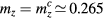 . At this point it is important to note that the transition between both phases is of first order, i.e. the magnetization changes discontinuously, as it is shown in figure 14. The average between the magnetization values right below and above the transition is approximately 0.24, which is in good agreement with our simple estimate.

Figure 14. Magnetization mz(H) curves obtained from the T = 0 variational approach and from the MC simulations at different finite temperatures.
Download figure:
Standard image High-resolution imageThe conclusion of this section is that easy-axis anisotropy can easily induce a skyrmion crystal right below the saturation field of a frustrated magnet. Unlike the case of the isotropic model [66], the skyrmion phase stabilized by easy-axis anisotropy survives in the long wave length limit  . Other multiple-
 orderings can also be obtained for smaller values of the anisotropy [75, 76]. The following three ingredients are enough to obtain field-induced multiple-
 ordering: (1) C6 symmetry, such as triangular and kagome lattices, (2) finite
  ordering due to competing interactions, and (3) easy-axis anisotropy. FexNi1−xBr2 [79], ZnxNi1−xBr2 [48], and an Fe monolayer on Ir(1 1 1) [80, 81] may be candidate materials to exhibit field-induced skyrmion crystal phase.
4. Frustration in itinerant magnets
4.1. Frustrated RKKY Hamiltonians
So far we have considered the effects of frustration in MIs, i.e. systems whose magnetic degrees of freedom are always localized. It is also interesting to consider the case of itinerant magnets. In this case we need to distinguish between two quite different situations: systems whose magnetic moments only arise from the spin or orbital degrees of freedom of the conduction electrons and systems that contain localized moments in addition to the magnetic degrees of freedom of the conduction electrons. While it is interesting to analyze the role of frustration in both systems, here we will mainly focus on the latter case, which describes the situation of many 4f and 3d-electron materials.
The small size of 4f-orbitals leads to the formation of localized magnetic moments when the energy of the f-orbitals is well below the Fermi level of the conduction electrons. Like in the case of MIs, double occupancy of the f-orbitals is suppressed by an intra-orbital Coulomb interaction, which is much larger than the hybridization between the f-orbital and the orbtials that generate the broad conduction band. The minimal model that describes this situation is the Kondo Lattice (KL) Hamiltonian:
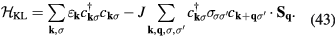
The operator  creates (annihilates) an itinerant electron with momentum
  and spin σ. The bare dispersion relation of the conduction electrons is
  , where tjl are hopping integrals between sites j and l. The second term of
  corresponds to the exchange coupling (J) between the conduction electrons and the localized magnetic moments in the momentum space representation
 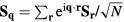 (N is the number of lattice sites). For the case of 4f-electron systems, J corresponds to the so-called Kondo AFM interaction. This model also applies to 3d-electron transition metal oxides, like the manganites [82], in which the localized moments are provided by t2g electrons, while the itinerant electrons occupy a band of eg-orbitals. In this case, J corresponds to the FM Hund's coupling between electrons in the same atomic shell. The energy gap separating the localized t2g-orbitals from the itinerant eg-orbitals is provided by the strong crystal field produced by the oxygen octahedron that surrounds the transition metal.
Here we will only consider the case of classical magnetic moments ( ), i.e. the
  limit. Although the Kondo effect disappears in this limit, we will still refer to
  as the KL Hamiltonian. The sign of J becomes irrelevant for classical moments because it can be absorbed by the transformation
  . Therefore, without loss of generality, we will assume that the coupling is FM.
In the weak-coupling regime,  , where
  is the density of states at the Fermi level
  , it is possible to integrate out the conduction electrons to produce an effective spin Hamiltonian up to second order in J. This procedure leads to the RKKY Hamiltonian
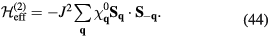
Here, 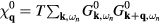 is the bare susceptibility of the conduction electrons,
 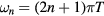 are the Matsubara frequencies, and
 ![$G_{\mathbf{k},{{\omega}_{n}}}^{0}={{\left\{i{{\omega}_{n}}-\left[{{\varepsilon}_{\mathbf{k}}}-\mu \right]\right\}}^{-1}}$](https://content.cld.iop.org/journals/0034-4885/79/8/084504/revision1/ropaa280aieqn384.gif) is the bare Green function (μ is the chemical potential). We note that
is the bare Green function (μ is the chemical potential). We note that  and
and 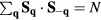 because of the local constraint
  . According to equation (44), any single-
 helical state whose ordering vector maximizes
  is a ground state of
  . This is the origin of the helical spin arrangements in rare-earth and other itinerant magnets that were identified towards the end of fifties and the beginning of sixties [8–10].
When  has a single global maximum,
  has a unique ground state up to global spin rotations. In contrast, the existence of multiple wave-vectors
  that maximize
  implies that
  has multiple ground states. In this case, we will say that the itinerant magnet is frustrated because there are many competing orderings. For instance, the circular Fermi surface (FS) of a 2D electron gas produces a highly-frustrated magnetic interaction:
  has a flat global maximum for
  and it decreases for
  (see figure 15(a)), implying that any
  -spiral ordering with
  is a ground state of
  .
.

Figure 15. (a) Bare magnetic susceptibility of a 2D electron gas.  depends only on
  in the absence of an underlying lattice because of space rotational invariance. For lattice systems with very small Fermi surfaces (
 ), the degeneracy of
  for
for  is removed by corrections of order k4 to the bare single-particle particle dispersion. (b) Example of four peak susceptibility
  for a square KL model. The ordering wave-vectors, ±
 (
( ), connect opposite points on the Fermi surface.
Download figure:
Standard image High-resolution image4.2. Non-coplanar orderings
The ground state degeneracy of  is removed by contributions of order J 4 and higher, which were neglected in going from
  to
to  . As we will see below, these contributions often select exotic magnetic orderings which are qualitatively different from a simple single- Q spirals. More importantly, the resulting multiple-
 orderings are in general non-coplanar, i.e. they have a non-zero scalar spin chirality:
  . This order parameter couples to the orbital degrees of freedom of the conduction electrons. The exchange interaction, J, tends to align the spins of the conduction electrons to the underlying local moment texture, inducing a Berry phase in the electron wave-function, which is indistinguishable from a 'real' magnetic flux (see figure 16). When conduction electrons propagate through such a spin texture, they may exhibit spontaneous Hall effect in the absence of any externally applied magnetic field [84]. Moreover, a spontaneous quantum Hall insulator can emerge from the chiral ordering if it gaps out the full Fermi surface [85–87].

Figure 16. When an electron moves around a loop jkl, it picks up a Berry phase. In the strong-coupling limit  , this Berry phase is equal to half of the solid angle,
  , subtended by the three spins in the loop [83]. This Berry phase can be associated to a Bohm–Aharanov phase produced by an effective 'magnetic flux'
  , where
  is the flux quantum. It is then clear that this real space Berry phase may change the topology of the electronic band structure (induce a Berry phase in momentum space) leading to the so-called topological Hall effect [84, 85].
Download figure:
Standard image High-resolution imageHere we will follow [88] to illustrate the role of frustration in the instability of single- spirals toward multiple-
 non-coplanar orderings. We start by considering the simple case of a square KL Hamiltonian (43), whose magnetic susceptibility has four global maxima connected by the C4 symmetry operations of the square lattice. This is a quite general situation for arbitrary band filling fractions, which typically leads to susceptibility maxima at low-symmetry wave-vectors. For the case under consideration, these wave-vectors are
  , with
  . We will also assume that these ordering wave-vectors connect opposite points on the FS.
We argue that the relevant variational ansatz is a double-Q vortex crystal state,
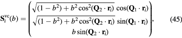
where  is the position vector of the site i. For b = 0, equation (45) describes an ordinary single-
 spiral in the xy spin-plane. A nonzero b introduces an out-of-plane (z component) modulation of amplitude b and wave vector
  , which deforms the single-
 spiral into a vortex crystal state, as it is shown in figure 17. This state also exhibits a one-dimensional modulation of the scalar chirality (chirality stripes) along the
  direction.

Figure 17. Vortex crystal described by equation (45). The colors indicate the out-of-plane (x) spin component (green for spin down orientation and red for spin up). The spin frame is rotated from equation (45) to show the vortex structure clearly. In this example, we chose  ,
,  with
with  , and b = 1. Vortices and antivortices are indicated with red and green colors, respectively.
Download figure:
Standard image High-resolution imageThe basic motivation for proposing this particular multiple- ordering is that the vector amplitude of the
  component is orthogonal to the vector amplitude of the
  -spiral. This condition guarantees that the amplitude of the higher harmonics required to enforce the constraint
  is of order b2, instead of the order b that would be obtained if the two vector amplitudes were not orthogonal to each other. As a consequence, this particular choice of multiple-
 ordering has an RKKY energy cost of order
  instead of
  .
.
The spin configuration of the vortex crystal in equation (45) has higher harmonics, which arise from an expansion of the square root prefactors introduced to satisfy the normalization condition  . This is true in general for any multiple-
 solution, as long as
  and
and  are not high-symmetry wave vectors. This observation implies that multiple-
 orderings have higher energy than the single-Q helical ordering at the RKKY level. However, as we will see below, the energy balance can change when higher-order terms are included.
The fourth-order contribution to the perturbative expansion in powers of J gives
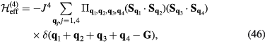
where  is the coefficient for the four-spin scattering process with momenta
  , and
, and  and
and  is a reciprocal lattice vector. Because we are interested in scattering processes involving the lowest energy modes
  , we only need to keep the contributions
  ,
, 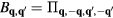 , and
, and 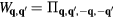 :
:
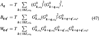
which correspond to the Feynman diagrams depicted in figure 18.

Figure 18. Feynman diagrams for the fourth order contributions listed in equation (47).
Download figure:
Standard image High-resolution imageIn the following we will assume that  . By Fourier transforming the spin configuration in equation (45) and substituting into equation (46), we obtain the energy up to
  :
:
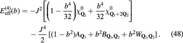
The energy difference between the proposed multiple- ordering and the single-
 spiral,
 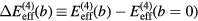 , is
, is
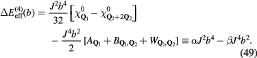
The coefficient α is always positive because  is maximized at
  . If β also turns out to be positive, the optimal value of b is
 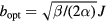 . Indeed, explicit evaluation of the coefficients
  ,
,  , and
, and  gives
gives  at a low enough T, as long as
  connects opposite points on the FS. Moreover,
  ,
,  , and
, and  diverge for
  . While this observation implies that the perturbative expansion is not valid in the
  limit, it suggests that b can become of order one even for very small J.
This hypothesis can be verified by introducing a regular (nondivergent) perturbative treatment. This approach requires to change the local reference frame for the spin components of the itinerant electrons. The local quantization x-axis is now aligned with the local moments of the single- helical state. The local moments of the double-Q non-coplanar vortex crystal become
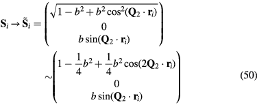
in the new reference frame. By applying the same transformation to the creation and annihilation operators of conduction electrons, we obtain:


Up to the quadratic order in b (we assume that  ), we obtain the following expression for
  with the local moment configuration given by equation (45):
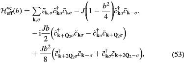
with  . This is a more adequate basis for applying perturbation theory because electronic scattering with the
  component of the spin configuration is accounted for exactly via direct diagonalization of the first two terms of
  . The divergence of the fourth-order contributions to the perturbative treatment in the original basis is avoided in this new basis because they are incorporated in second order contributions in the amplitude of the last two terms of
  [88].
[88].
The most significant second-order contributions to the total energy arise from the regions around the two pairs of FS points (hot spots) connected by the ordering vectors  and
and  (see figures 19(a) and (b)). The dispersion around these points can be parametrized in terms of the Fermi velocity, vF, and the radius of curvature R0 of the FS. Here we are assuming that
  , i.e. that the Fermi segments connected by
  are close to be nested.
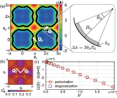
Figure 19. (a) FS (black curves) and energy dispersion  (contour plot) for t3 = −0.5, J = 0, and
  in an extended BZ.
  and
and  are the wave-vectors that maximize the bare susceptibility,
  , shown in panel (b). In the enlarged figure, we show the way in which the FS is approximated near the hot spots. We use cylindrical coordinates (R0,
  ) for evaluating the result of perturbation theory (see the text). (c) Energy of multiple-
 solution proposed in equation (45) with
  as a function of b2 for t3 = −0.5, J = 0.1, and
  . The results were obtained for a finite lattice of N = 9602 sites. The circles and squares show the results obtained from the perturbative approach and from an exact evaluation the energy by using direct diagonalization, respectively. Exact diagonalization is possible for
  because the magnetic unit cell is not too large.
Download figure:
Standard image High-resolution imageThe change in energy induced by a nonzero b value (out-of-plane component) has a positive contribution (energy cost),  , arising from the first two terms of equation (53) and a negative contribution (energy gain),
  , that arises from the last two terms of the same equation. By following the procedure described in [88], we obtain
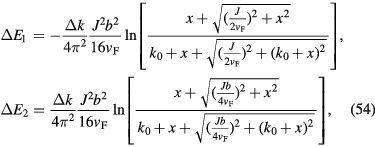
where  and k0 define the circular rectangle of integration around the hot spots (see figure 19(a)), and
 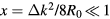 . By adding the energy cost and the energy gain, and expanding in small J and b, we obtain that the leading order contribution is
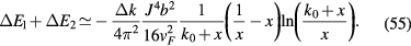
It is clear that  in the region where the perturbative approach is valid (
 ). Moreover, we have found that the energy difference between the vortex crystal state and the single-
 ordering is of order
  for small J and b. This result agrees with our naive expectations based on equations (48) and (49). However, we have arrived to this result without encountering any divergence on the way.
Equation (54) reveals the origin of the non-coplanar magnetic ordering: the single- state still has a high susceptibility for developing an additional
  modulation. In particular, this susceptibility is logarithmically divergent in the limit of perfect nesting (
 ), i.e. the energy gain
  becomes proportional to
  , while the energy cost
  remains proportional to b2.
Figure 19(c) shows the E(b) curve obtained from our perturbative approach after integrating over the  (not just around the hot spots). For small b values, E(b) is in good agreement with the exact evaluation for the double-Q state in equation (45), which can be computed by direct diagonalization of
  when the magnetic unit cell associated with the wave-vectors
  is not too large. A deviation
  (
( ,
,  ,
,  ) for b = 0.1 is consistent with the expected accuracy of the perturbative expansion. The stabilization of the non-coplanar vortex crystal described by equation (45) has been confirmed with unbiased Langevin dynamics simulations [88].
The above analysis shows that contributions which are not included at the RKKY level can radically change the nature of the magnetic ordering of frustrated itinerant magnets. In particular, these terms favor multiple- non-coplanar magnetic orderings which, in turn, produce an effective spin–orbit coupling via the Berry phase mechanism that was discussed at the beginning of this section. In particular, the chirality stripes of the non-coplanar vortex crystal described by equation (45) produce staggered electronic currents in the direction parallel to the stripes. The purpose of the next section is to show that the stabilization mechanism discussed here leads to other interesting non-coplanar magnetic orderings for special filling fractions.
4.3. Anomalous Hall effect
The FS of the half-filled square lattice with nearest-neighbor hopping is a perfect square inscribed into the bigger square boundary of the first Brillouin zone (see figure 20(a)). This implies that the Fermi surface is perfectly nested with a single nesting wave-vector  . The corners of the square correspond to saddle points of the dispersion relation
  , implying that the density of states diverges logarithmically at these points (Van-Hove singularity). The combination of perfect nesting and the Van-Hove singularity leads to magnetic susceptibility
  that diverges as
  . Naturally, this divergence is stronger than the
  divergence of the uniform susceptibility, which is proportional to the density of states. Therefore, as it is shown in figure 20(a), the dominant magnetic ordering for the weak-coupling regime of the half-filled square KL model (KLM) is a plain collinear antiferromagnet with ordering wave-vector
  . Frustration is absent in this example because the magnetic susceptibility has a single global maximum.

Figure 20. (a) FS of the half-filled square lattice tight-binding Hamiltonian with nearest neighbor hopping. The perfect nesting at  leads to the collinear two-sublattice AFM ordering shown in the figure for the weak-coupling regime of the KLM (43). (b) FS of the three quarters-filled triangular lattice tight-binding Hamiltonian with nearest-neighbor hopping. In this case there are three nesting wave-vectors
  with
with  and the preferred ordering is the 3-
 non-coplanar ordering that is shown right next to the FS.
Download figure:
Standard image High-resolution imageWe will consider now the case of the three-quarter filled triangular lattice with nearest-neighbor hopping [86]. Similarly to the case of the half-filled triangular lattice, the FS consists of a prefect regular hexagon that is inscribed in the bigger hexagonal boundary of the first Brillouin zone (see figure 20(b)). However, in contrast to the square lattice case, the hexagonal FS has three nesting wave-vectors  with
with  . Like in the previous case,
  are half of reciprocal lattice vectors and the corners of the FS are saddle points of
  . Consequently, the magnetic susceptibility diverges at each of these wave-vectors as
  , i.e. it has three degenerate global maxima. Given the frustrated nature of the magnetic susceptibility, it is natural to ask what is the optimal magnetic ordering.
To answer this question we will first consider the RKKY Hamiltonian  given in (44). It is clear that a ground state of
  cannot have
  -components different from
  . Consequently, the ground-space of
  is parametrized by the following expression:
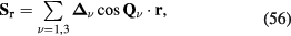
where  are the vector amplitudes of the three wave-vectors
  . The normalization condition of the local classical moments,
  , implies that these vector amplitudes cannot take arbitrary values. Given that the wave vectors
  are half of reciprocal lattice vectors, the normalization condition implies that the three vector amplitudes,
  , have to be orthogonal to each other:

This condition leaves us with three possible orderings: (a) collinear ordering if two vector amplitudes are zero; (b) coplanar ordering if one vector amplitude is zero; and (c) non-coplanar ordering if the three vector amplitudes are non-zero. As it can be anticipated from the discussion in the previous section, direct evaluation of the exact energy of  for these three states shows that the non-coplanar ordering with
  is the actual ground state [86].
Figure 21(b) shows that the real space version of the 3- non-coplanar magnetic ordering is a four-sublattice structure in which the spins of each sublattice point towards each of the four corners of a regular tetrahedron. In particular, the solid angle subtended by three spins from the same triangle jkl is one quarter of the full solid angle of the sphere, i.e.
  , as it is shown in figure 21(c). Correspondingly, the Berry phase that electrons pick up when they move around each triangle is
  . In other words, each triangle acquires a uniform spontaneous net 'magnetic flux'
  equal to one quarter of the flux quantum
  . The real external magnetic field that would be required to produce such a flux is 104T if we assume that the lattice parameter is of the order of a few Angstroms. Interestingly enough, Akagi and Motome found the same magnetic ordering for the intermediate-coupling regime of the quarter-filled (n = 1/4) KLM [89, 90].

Figure 21. (a) Fermi surface for a triangular lattice with nearest-neighbor hopping at filling fraction n = 3/4 and the nesting wave vectors,  , which are equal to reciprocal lattice vectors. (b) The 3-
 magnetic ordering that arises from Fermi surface nesting corresponds to a 4-sublattice structure in which the spins of each sublattice point towards each of the four corners of a regular tetrahedron. (c) The solid angle subtended by three spins from the same triangle jkl is one quarter of the full solid angle of the sphere, i.e.
  .
.
Download figure:
Standard image High-resolution imageMermin–Wagner's theorem [78] precludes long-range magnetic ordering at finite T because it breaks the continuous SU(2) symmetry of  . In contrast, the scalar spin chirality
  breaks only discrete symmetries, such as time-reversal and mirror symmetries. Therefore, in contrast to the magnetic ordering, long range chiral ordering can persist up to a finite critical temperature. MC and Langevin Dynamics simulations of
  for filling fractions n = 1/4 (intermediate coupling) and n = 3/4 (weak-coupling) show that this is indeed the case, and that the chiral ordering disappears through a first order thermodynamic phase transition [87, 91]. Like in the case of Mott insulators, the local physical observable associated with the scalar spin chirality is the orbital contribution to the magnetization, i.e. the component associated with orbital motion of the conduction electrons under the presence of the local effective flux
  . In particular, given that the triple-
 state that we are considering has a uniform scalar spin chirality, the global order parameter is the uniform orbital magnetization, i.e. the chiral spin liquid is just an orbital ferromagnet.
The transverse or Hall conductivity,  , is a non-local physical property that can also be used to characterize the chiral liquid state of an itinerant magnet. The uniform effective flux should naturally induce a finite
  . This phenomenon is known as anomalous Hall effect (AHE) and it has been studied for many years [92]. However, most of the original proposals for finding AHE in real materials relied on the relativistic spin–orbit interaction, as a key mechanism for stabilizing the non-coplanar magnetic orderings required to produce the emergent gauge field
  . As we are showing in this section, magnetic frustration is an alternative route to induce AHE even in absence of relativistic spin–orbit coupling.
For the case under consideration, the uniform effective flux is induced by a non-coplanar ordering that fully gaps out the original Fermi surface. This implies that the Hall conductance must be quantized [93]. The value of  can be anticipated by using the following trick. We will assume that the local moments remain in the 'tetrahedral'
  ordering depicted in figure 21, while we adiabatically increase the coupling constant J all the way to the strong coupling regime
  . It is clear that the gap only increases along this process, leading to two disconnected sectors in the strong-coupling limit: the low (high) energy subspace of states in which conduction electrons hop between neighboring sites remaining parallel (anti-parallel) to the local moment
  .
.
The overall energy splitting between these two sectors is 2JS. Within each sector, the conduction electron spin orientation is now enslaved to the orientation of the local moment. This implies that the effective Hamiltonian that results from projecting  onto the low (high)-energy subspaces consists of spinless fermions with an effective hopping

where  is the solid angle subtended by the local moments on the sites j and l, and a unit vector
  associated to each triangle jkl. Here we only need to consider half of the triangles (let's say the triangles that point upwards) because each bond belongs to two triangles. The variable σ denotes the relative orientation between the spin of the itinerant electron and the local moment, i.e.
  (−1) for the low (high) energy subspaces. The arbitrary choice of the unit vectors
  corresponds to the gauge freedom of this effective low-energy theory known as double-exchange model [94]. We note that the circulation of the the phase,
 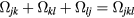 , is equal to twice the gauge invariant flux of the triangle jkl, which turns out to be equal to the solid angle subtended by the local moments
  ,
,  and
and  , as we already anticipated in the previous section (see figure 16). As we anticipated in figure 16, this phase indistinguishable from the Aharonov–Bohm phase that an electron would pick up in an externally applied magnetic field [95].
For the specific case of 'tetrahedral' ordering that we are considering (see figure 21), we have
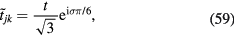
when we circulate clockwise (from j to k) around a triangle jkl that is pointing upwards. Here we are using a particular gauge choice in which the unit vectors  are parallel to the sum of the three moments j, k and l.
For the specific case of the 'tetrahedral' ordering shown in figure 21, the solid angle subtended by local moments in corners of each elementary triangular plaquette is clearly  . Thus, in the limit of strong coupling, the problem is equivalent to one of spinless electrons on a triangular lattice in a uniform spin-dependent magnetic field that produces a flux
  per triangular plaquette. The energy spectrum in the strong-coupling limit is
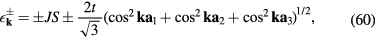
where  and
and  are real space lattice vectors of the triangular lattice and
  . Since the real space (magnetic) unit cell has doubled, this dispersion is defined on half of the original Brillouin zone. There are total of four energy-split bands. Thus, the system is an insulator for fillings that are integer multiples of 1/4. Filling n = 1/2 corresponds to full filling of the spin-up sector, and therefore it is equivalent to a band insulator with
  . From the explicit treatment of spinless electrons on triangular lattice [96], one finds that
  for the filling fraction n = 3/4 that we are considering here. This result is not surprising considering that four triangles contain one flux quantum for the tetrahedral ordering shown in figure 21, and that n = 3/4 corresponds to one hole per two sites, i.e. one hole per flux quantum. As we mentioned before, the same magnetic ordering is obtained at n = 1/4 for intermediate-coupling. In this case we just need to occupy the lowest energy band of spin-up sector. Clearly we still have
  because in this case we have one electron per-flux quantum. However,
  has an opposite sign in this case because spin up and down electrons experience opposite fluxes.
Because the gap does not close when we reduce J all the way from the strong to the weak-coupling limit, relevant for n = 3/4,  remains equal to e2/h. This can be verified by explicit calculation of the Kubo formula directly in the weak-coupling regime [86]. In other words, the insulator that is induced by the tetrahedral ordering depicted in figure 21 is a Chern insulator. This phenomenon is known as quantum anomalous Hall effect (QAHE).
Our simple example of 3- in the triangular lattice clearly shows that spontaneous non-coplanar magnetic orderings can be exploited to modify the topological properties of the reconstructed bands and for instance induce QAH effect at ambient temperature [87]. As we explained in the previous section, magnetic frustration is reflected in the multiple wave-vectors that maximize the electronic susceptibility. By now there are several examples of non-coplanar orderings that produce QAH effect for different lattices and filling fractions [85, 89, 97–107]. It has also been shown that a QAH state can naturally arise form KL Hamiltonians of itinerant electrons interacting with chiral ice states of local moments, such as Kagome ice [103, 108]. The robustness of the QAH state against thermal fluctuations that do not destroy the chiral ordering of the local moments is a direct consequence of the robustness of the integer quantum Hall state against disorder. It is interesting to note that the QAH state can be suppressed by application of an external magnetic field. The Zeeman coupling between the field and the local moments favors a fully polarized state, implying that the charge gap must close at critical value of the field [87].
The non-coplanar four-sublattice ordering that we discussed in this section (see figure 21) has been proposed to describe the magnetic ordering in Mn monolayers on Cu(1 1 1) surfaces [109]. In general, non-coplanar magnetic orderings have been recently observed in 2D layers of 3d metals deposited on a nonmagnetic metallic surface [81, 110]. Moreover, first-principles calculations for these systems [109–110] indicate that these non-coplanar orderings arise from rather strong effective four-spin interactions. The results that we discussed in this section unveil the generic origin of these effective interactions and explain why they are so ubiquitous in frustrated itinerant magnets.
5. Conclusions
In the previous sections we have reviewed a few examples of novel phases and responses enabled by frustration. These simple examples reveal that frustration is a natural guiding principle in the search for novel physical phenomena. In particular, we have seen that complex states of matter, such as chiral magnetic orderings and chiral liquids, can naturally emerge from frustration both in localized and in itinerant magnets. Given that scalar chirality has the same symmetry properties as an orbital magnetic moment, it is not surprising that chiral orderings induce loop currents both in Mott insulators and in itinerant magnets. As we have seen here, this effective coupling between spin and charge degrees of freedom can produce unusual physical phenomena, such as spontaneous QAH states induced by chiral liquids, or just orbital currents for the case of Mott insulators. The possibility of having orbital currents in Mott insulators implies that the electronic charge density can also get redistributed because the current and charge density operators are related by the continuity equation. We have seen that this electronic charge modulation is associated with bond orderings (bond operators have the same symmetry properties as particle density operators). This simple phenomenon enables giant magneto-electric effects of pure electronic origin triggered by spontaneous bond orderings in Mott insulators. Like in the case of chiral orderings, bond orderings can exist with or without magnetic ordering. Examples of strong magneto-electric effects induced by both types of orderings have been recently found in an organic Mott insulator [111].
The chiral magnetic orderings that we described in this article include magnetic superstructures, such as vortex or skyrmion lattices, with characteristic length scales which are controlled by the ratio between the two competing exchange constants, in the case of Mott insulators, and by the magnitude of the Fermi wave vector in the case of itinerant systems. This length can vary from a few atomic spaces to the mesoscale, depending on the material under consideration. In particular, skyrmions have recently captured the attention of the condensed matter community because of their potential technological relevance. In contrast to the case of skyrmions induced by competition between FM exchange and DM interaction, skyrmions induced by frustration have an internal (chiral) degree of freedom that could be exploited for memory applications.
We have also seen that non-magnetic impurities can nucleate magnetic vortices above the saturation field of frustrated quantum or classical magnets with competing FM and AFM exchange interactions. Vortices commonly appear in other bosonic systems, such as superconductors and atomic Bose gases, under the application of magnetic field, in the case of charged systems, or induced by rotation of a neutral condensed gas. Here we showed that vortices can also appear in frustrated magnets around the 'hole' created by a non-magnetic impurity. Moreover, we have seen that periodic inhomogeneous structures, such as charge density waves, can stabilize vortex lattices near the saturation magnetic field and other exotic chiral orderings across the whole field-temperature phase diagram. Here we have only considered the simple case of commensurate length scales for the magnetic and the CDW orderings. More complex spatially modulated chiral magnetic superstructures can be obtained when both length scales are not commensurate with each other.
Finally, we have shown that effective four and higher spin interactions can be rather strong in itinerant magnets. As a consequence, the single- magnetic ordering that is naively expected from the RKKY effective Hamiltonian is not always the ground state of the original Kondo Lattice model. In particular, we have seen that this is the case for C4 frustrated itinerant magnets with four peaks in the magnetic susceptibility at symmetry related wave-vectors
  (
( ). This observation can be directly extended to more general frustrated itinerant magnets with susceptibility maxima at multiple symmetry related wave-vectors connecting opposite points of the FS. This weak-coupling instability suggests that frustrated itinerant magnets are natural candidates to exhibit non-coplanar multiple-
 magnetic orderings, which go beyond the simple single-
 helical orderings that were originally proposed based on the oversimplified RKKY model.
In all the cases considered in this manuscript, the scalar chiral liquids were induced by thermal fluctuations that destroy the magnetic LRO, but preserve the broken discrete symmetries associated with a non-zero local scalar chirality  . Similar chiral liquids can in principle be stabilized at T = 0 via quantum fluctuations. This is a quite common situation in one-dimensional systems (continuous symmetries are preserved at T = 0 in most cases), that could also arise in highly frustrated 2D and 3D systems. This is an exciting pathway for future research in this area.
Acknowledgments
We thank A Chubukov, Y Motome, R Ozawa, I Martin, G-W Chern, K Barros, A Rahmani, L Bulaevskii, and J Venderbos for very useful discussions. YK acknowledges the financial support from the RIKEN iTHES project. Work at LANL was carried out under the auspices of the U.S. DOE contract No. DE-AC52-06NA25396 through the LDRD program.
Appendix.: Effective operators in Mott insulators
A.1. Effective charge operator
Equation (9) shows the functional form of the effective charge operator  to
to  for the strong-coupling limit of the hall-filled Hubbard model. As we discussed in the main text, this contribution from the smallest loop of frustrated lattices that is a triangle (jkl) (see figure A1(a)). Below we derive the proportionality constant
 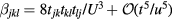 in this expression. To this end, it is sufficient to evaluate a particular nonzero matrix element on both sides of
 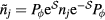 by choosing a convenient basis set. Here we consider the subspace characterized by (1) the total spin S = 1/2, (2) Sz = 1/2, and (3) even parity under exchanging k and l, i.e.
  , and
, and  . The corresponding basis states are (see figure A1(b))
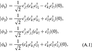
where only  is a pure spin state with
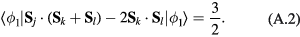

Figure A1. (a) Three-site loop on the triangular lattice and (b) and (c) unperturbed basis sets we use to fix the prefactors in the effective charge and current operators, respectively.
Download figure:
Standard image High-resolution imageFor the moment we assume  and denote the kinetic term in
  as
as  . The matrix elements of
  and
and  are represented, respectively, as
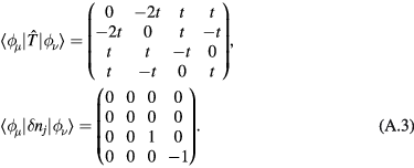
We denote the unperturbed Hamiltonian as 
 where a chemical potential term to ensure the half-filling has been included. By denoting
 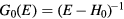 and
and  , we compute
  to
to  as follows by using perturbation theory:
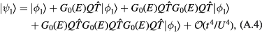
where
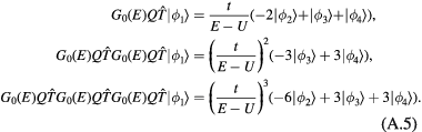
In fact we will not use the last piece because  is diagonal in the present basis set. We obtain
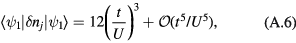
which we should compare with  (see equations (9) and (A.2)). Thus we conclude
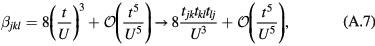
where in the last line we have recovered the bond dependence of the hopping integrals, the correctness of which can be suggested by the fact that we have computed the lowest order  term arising from a triangular loop.
A.2. Effective current operator
Next we discuss how to determine the prefactor  that appears in the effective current operator (equation (8)). For this purpose, the above basis set
  –
–  is not appropriate because
 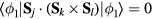 . Instead, we use a different basis generating a chiral subspace characterized by (1) S = 1/2, (2) Sz = 1/2, and (3) the eigenvalue
  under the C3 rotation (see figure A1(c)):
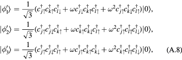
where only  is a pure spin state and
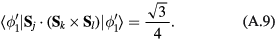
By using the matrix elements of  and
and 
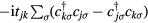 , namely,
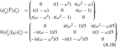
respectively, we evaluate  perturbatively in the same way as in equation (A.4). We obtain
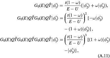
and thus,
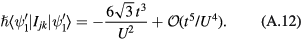
By comparing this with equation (A.9), we conclude
where we have recovered the bond dependence on the hopping integrals.
Footnotes
- 1
22 provides a similar argument but only for the continuum limit (
 ).
).
