

Abstract
Accurate activity quantification is the foundation for all methods of radiation dosimetry for molecular radiotherapy (MRT). The requirements for patient-specific dosimetry using single photon emission computed tomography (SPECT) are challenging, particularly with respect to scatter correction. In this paper data from phantom studies, combined with results from a fully validated Monte Carlo (MC) SPECT camera simulation, are used to investigate the influence of the triple energy window (TEW) scatter correction on SPECT activity quantification for  Lu MRT.
Results from phantom data show that; (1) activity quantification for the total counts in the SPECT field-of-view demonstrates a significant overestimation in total activity recovery when TEW scatter correction is applied at low activities ( 200 MBq). (2) Applying the TEW scatter correction to activity quantification within a volume-of-interest with no background activity provides minimal benefit. (3) In the case of activity distributions with background activity, an overestimation of recovered activity of up to 30% is observed when using the TEW scatter correction.
Data from MC simulation were used to perform a full analysis of the composition of events in a clinically reconstructed volume of interest. This allowed, for the first time, the separation of the relative contributions of partial volume effects (PVE) and inaccuracies in TEW scatter compensation to the observed overestimation of activity recovery. It is shown, that even with perfect partial volume compensation, TEW scatter correction can overestimate activity recovery by up to 11%. MC data is used to demonstrate that even a localized and optimized isotope-specific TEW correction cannot reflect a patient specific activity distribution without prior knowledge of the complete activity distribution. This highlights the important role of MC simulation in SPECT activity quantification.
Export citation and abstract BibTeX RIS

Original content from this work may be used under the terms of the Creative Commons Attribution 3.0 licence. Any further distribution of this work must maintain attribution to the author(s) and the title of the work, journal citation and DOI.
1. Introduction
Molecular radiotherapy (MRT) is an established procedure in which radiolabelled pharmaceuticals are administered to a patient in order to deliver a targeted therapeutic radiation dose to malignant cells whilst sparing healthy tissue. There is now an extensive clinical portfolio of MRT procedures. A clinical treatment regimen, as an example Peptide Receptor Radionuclide Therapy with  Lu-Dotatate, may include pre-treatment imaging with a diagnostic radionuclide labelled pharmaceutical, for example
  In-Octreotide or 68Ga-Dotatate. This is followed by a fractionated delivery of a therapeutic radio-pharmaceutical with accompanying post administration imaging. To optimize MRT and patient outcomes, radiation doses to tumour and organs at risk should be accurately determined for each patient using nuclear medicine imaging. Such patient specific dosimetry is now regarded as an essential requirement for MRT (Bardiès et al 2006) and the basis of this dosimetry is accurate spatial and temporal activity quantification. Accurate activity quantification for MRT presents a unique challenge due to the requirement of detecting radiation emissions from internal particle and gamma decay emissions. In addition, time-activity data for MRT is highly patient-specific and varies significantly for different organs and tumour burdens, often requiring detailed pharmacokinetic modelling (Brolin et al 2015). Consequentially, the related image corrections used to generate quantitative nuclear medicine images must be applied across a wide range of activities, from MBq to GBq.
Single photon emission computed tomography (SPECT) is the most common form of imaging used with MRT, often with concurrently acquired cross-sectional anatomical imaging. Activity quantification from SPECT images commonly requires the measurement of a sensitivity standard containing a known activity. The choice of concentration, volume and medium in which the known activity is contained can compensate for many camera system specific effects, such as partial volume recovery artifacts (Jaszczak et al 1981, Rosenthal et al 1995). This approach to SPECT calibration, whilst sub-optimal compared to applying individual quantitative corrections for these effects, is often applied clinically and has been shown to compensate for imperfect scatter and attenuation corrections (Dewaraja et al 2012). A variety of scatter correction methods have been developed for SPECT imaging (Hutton et al 2011). Many of these methods have focused primarily on providing improvements to the contrast and spatial resolution of the image for image interpretation purposes rather than on providing accurate activity quantification for patient dosimetry. The identification and subtraction of the true number of photons which undergo scatter and lose some energy before entering the detector still presents a major challenge to obtaining accurate quantification from SPECT images.
The triple energy window (TEW) scatter correction method (Ogawa et al 1991) is a technique commonly used to compensate for scattered photons when processing SPECT images. This technique uses upper and lower scatter energy windows, immediately adjacent to the photopeak window, to estimate the number of scattered photons and is based on the position dependent scatter correction method of Koral et al (1988). In the work of Ogawa et al (1991) the optimal location and width of the photopeak and scatter windows were determined using a Monte Carlo (MC) simulation of an idealized 99mTc SPECT phantom. The choice of windows was initially validated by considering profiles of the reconstructed phantom. The validity of the TEW method was further evaluated for myocardial studies with 99mTc,  Tl and
  I (Ichihara et al 1993) using the same window definitions to assess the quantification of phantom data.
With the recent increase in the number of MRT radionuclides and therapy options, there is an enhanced need for image quantification methods which can provide accurate data for patient specific dosimetry across the range of therapies.  Lu-Dotatate is an important MRT agent (Kwekkeboom et al 2008) which is increasingly being used for therapy of neuroendocrine tumours (NET). The decay of
  Lu and de-excitation of its daughter nucleus
  Hf results in the emission of two gamma rays of energy 113 and 208 keV and a beta-decay with an average energy of 147 keV (Kondev 2003). This combination of beta emission for therapy and multiple gamma ray emissions for imaging gives the potential for assessment of MRT efficacy. However the quantification accuracy of
  Lu is limited by its complex emission spectrum. Figure 1 shows (a) the simple single peak emission spectrum for 99mTc in contrast to (b) the more complex multiple emission spectrum of
  Lu for a water filed phantom measured with a Infinia-Hawkeye-4 SPECT/CT (GE Healthcare) camera.
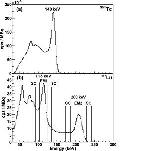
Figure 1. Emission spectrum for a water filled phantom measured with an Infinia-Hawkeye-4 SPECT camera for (a) 99mTc with low energy high resolution (LEHR) collimator and (b)  Lu with medium energy general purpose (MEGP) collimator. The standard TEW correction photopeak emission (EM) and adjacent scatter (SC) windows for
  Lu are indicated by vertical lines. Note the increased complexity of the emission spectrum for
  Lu, with its two emission lines, in comparison to 99mTc.
Download figure:
Standard image High-resolution imageThe recently published MIRD guidelines for quantitative  Lu SPECT (Ljungberg et al 2015) recommend applying the TEW scatter correction, as defined in Ogawa et al (1991), to provide an estimate of scattered photons. It is important to note that this selection of windows for
  Lu TEW scatter correction is not optimized for its complex emission spectrum. A comparison of energy window subtraction-based scatter correction methods for
  Lu is given in de Nijs et al (2014). The validity of the TEW scatter correction for
  Lu is of particular concern for the lower 113 keV gamma ray emission which has a significantly increased scatter fraction (from down scatter of the 208 keV emission) in contrast to both the single gamma emitter 99mTc and the 208 keV emission in
  Lu (see figure 1). This has lead to a number of clinical centers using the 208 keV emission peak only, with a consequential loss of detector sensitivity. MC simulation is being increasingly used to study the interaction of gamma rays in SPECT camera systems (Hutton et al 2011) and for complex emission spectra, such as from
  Lu, is often the only way to obtain a complete understanding of the gamma ray scattering interactions.
In this paper we have assessed the influence of the TEW scatter correction on the activity quantification of  Lu SPECT images. Phantom data, together with a MC simulation of an Infinia-Hawkeye-4 SPECT/CT system, were used to compare activity recovery factors measured using a clinical protocol. A range of tumour to background activity ratios and imaging time points corresponding to a typical
  Lu-Dotatate patient therapy were considered. By using identical phantom data for calibration and imaging, the performance of the relative calibration factor (Dewaraja et al 2012, Ljungberg et al 2015) is maximised and the influence of the TEW scatter correction is isolated from other imaging and reconstruction artifacts. The unique ability of the MC simulation to track the interaction history of gamma rays was used to determine the contribution of increased partial volume effects, allowing the influence of the TEW correction to be fully isolated. The limits to quantitative accuracy for a TEW based scatter correction method, with a pragmatic upper limit on the length of a SPECT acquisition, for
  Lu MRT are evaluated.
2. Methods
2.1. Triple energy window (TEW) scatter correction
The 2D projected spatial distribution of scattered photons  in an energy window centered on the photopeak of a gamma ray emission can be estimated using additional projection data from adjacent scatter rejection windows (Ogawa et al 1991).

where, wp is the width of the emission (EM) photopeak, wl and wu are the widths of the adjacent lower and upper scatter windows in keV and Cl and Cu are the counts in the corresponding scatter windows. During a typical clinical acquisition a photopeak width of ±10 and SC windows of ±3
 are used for both EM1 (113 keV) and EM2 (208 keV), as indicated in figure 1(b). Projections corresponding to EM1, EM2 and the adjacent scatter windows are acquired simultaneously. A projection image data set corresponding to the estimated scatter from the TEW, is then calculated using equation (1). For optimal performance the scatter estimate should be incorporated into the projector step in an iterative reconstruction algorithm (Hutton et al 2011). This is commonly not possible with manufacturer provided reconstruction software, in which case the scatter estimate is subtracted from the corresponding photopeak projection before reconstruction.
2.2. Phantom studies
A series of phantom experiments were performed using a cylindrical water filled phantom (7.3 l, 216 mm diameter and 200 mm height) with cylindrical inserts containing  Lu. The phantom was scanned with (BG) and without (No BG) activity in the body of the phantom. Three 10 ml cylinder phantom inserts (25 mm diameter, 20 mm height) contained activities covering a range of tumour-to-background activity ratios to represent typical clinical MRT imaging data (see table 1 for details). The phantoms were scanned at five time points, providing a range of total activities, as the
  Lu decayed. For all scans the phantom was placed in the center of the field-of-view of the SPECT camera. Projection images were acquired for energy windows corresponding to the
  Lu 113 keV photopeak (EM1), 208 keV photopeak (EM2) and for adjacent scatter windows, as described in table 2. The data were acquired using an Infinia-Hawkeye-4 SPECT/CT camera with medium energy general purpose (MEGP) collimators and acquisition parameters corresponding to a clinical
  Lu-Dotatate post-therapy scan (see table 2). In addition a pulse-height analysis (PHA) measurement of the energy spectrum for a fixed camera head position was acquired for each scan. Two additional calibration phantom scans; (1) a single 10 ml cylinder containing 226 MBq of
  Lu in a water filled cylindrical phantom (small volume sensitivity—SVS) and (2) 3551 MBq of
  Lu in the body of a cylindrical phantom with no inserts (whole body sensitivity—WBS) were performed. The calibration data were acquired using the same acquisition parameters (table 2) and used to provide separate calibration factors for small and large volume data with and without TEW scatter correction applied.
Table 1. Details of the cylindrical water filled phantom studies, containing three 10 ml cylinders, performed with an Infinia-Hawkeye-4 SPECT camera
| Experiment name | Phantom body activity (MBq) | Activity per insert (MBq) |
|---|---|---|
| No BG |
0 | 255.6, 253.3, 244.8 |
| No BG | 0 | 137.2, 136.0, 131.4 |
| No BG | 0 | 59.3, 58.9, 56.9 |
| No BG | 0 | 15.3, 15.2, 14.7 |
| No BG | 0 | 7.4, 7.3, 7.1 |
| BG |
2056 | 10.4, 35.6, 63.4 |
| BG | 992 | 5.0, 17.2, 30.6 |
aTomographic data acquired using parameters detailed in table 2. bNo background activity in phantom. cBackground activity in phantom.
Table 2. SPECT tomographic acquisition parameters corresponding to  Lu MRT patient scan.
| Pixels |  |
|---|---|
| Head mode | H |
| Rotation radius | 25 cm |
| Time per position | 40 s |
| Total positions | 30 (60 views) |
| Collimators | Medium energy (MEGP) 1 512 103 mm hexagonal holes, 58 mm depth |
| Standard photopeak Windows (keV) |  (EM1), (EM1),  (EM2) (EM2) |
| Standard scatter Windows (keV) |  , ,  , ,  , ,  |
2.2.1. Reconstruction.
The phantom data were reconstructed using a clinical OSEM reconstruction algorithm (GE OSEM) with 10 subsets and 4 iterations on a GE Xeleris 2 workstation. Narrow beam attenuation correction (AC) was applied with the Xeleris 2 workstation, using Hawkeye CT data acquired as part of the scan protocol. The use of attenuation maps generated from CT imaging using the camera manufacturer's own software for attenuation correction for  Lu is highly recommended (Ljungberg et al 2015). The SPECT data were reconstructed with parameters corresponding to a clinical protocol for
  Lu MRT dosimetry. Data were reconstructed for individual photopeaks (EM1 and EM2) with (1) AC and no scatter correction (AC) and (2) AC and the standard TEW scatter correction (AC)(TEW) applied prior to reconstruction. The application of scatter correction outside of the reconstruction algorithm, whilst sub-optimal, is a common procedure in commercial clinical reconstruction algorithms. A Hann prefilter (0.9) and Butterworth low-pass post-reconstruction filter with order 10 and normalized cutoff frequency 0.5, were applied to all reconstructed images. It should be noted that any filtering is generally applied based on the specific objectives of the study and will have an effect on quantification and partial volume contributions.
2.2.2. Phantom activity quantification.
A calibration factor, cf, can be defined which relates the count rate (counts per second, cps) in a reconstructed SPECT image to the known total activity (MBq) in a phantom or insert,

The whole body sensitivity (WBS) phantom measurement was used to determine calibration factors for the total counts in the SPECT camera field-of-view. The small volume sensitivity (SVS) phantom measurements were used to determine calibration factors for a volume-of-interest (VOI) corresponding to a 10 ml phantom insert. A VOI defining the 10 ml phantom insert was manually outlined using the Hawkeye CT data and transferred to the SPECT image. Partial volume effects in the final reconstructed images, leading to the loss of apparent activity due to the limited resolution of the SPECT camera, can be compensated for by using a sensitivity factor specific to the volume in which the activity is being quantified (Dewaraja et al 2012). This approach is typically used in clinical protocols. Whilst an anatomy based partial volume correction can provide a more robust approach, there is currently no widely accepted, well-validated method (Dewaraja et al 2012). In the present work, the SPECT images for calibration used the same reconstruction, attenuation correction and TEW scatter correction parameters as were used for the images being quantified to ensure accurate activity quantification.
For a known activity in a phantom volume an activity recovery factor (RF) is defined as,

where Aadmin is the known administered activity in a phantom volume and Aquantified is the quantified activity calculated for a specific calibration factor (equation (2)) appropriate to the volume being considered. Thus, for a specific calibration factor (cf) a recovery factor less than 1.0 corresponds to an underestimation of the quantified activity in the phantom, whilst conversely values greater than 1.0 represent an overestimation of the administered activity.
2.2.3. SPECT camera dead time.
The count losses due to dead time in a SPECT camera system for  Lu are small due to the low yield of gamma rays from the decay of
  Lu. Dead time effects are highly camera-specific and must be corrected for each individual photopeak and projection before reconstruction. The total activities used in this work were selected to be below the level at which deadtime effects are observed for the camera system used in this work (>2.5 GBq total activity).
2.3. Monte Carlo simulation
The GATE 6.1 (geant4 application for tomographic emission) (Jan et al 2004) package was used to develop a highly detailed simulation of the Infinia-Hawkeye-4 SPECT/CT camera. The details of the camera model used in the simulation are shown in figure 2. It has been shown (Rault et al 2011) that an accurate description of the back compartment, or alternatively a generic model of the compartment (glass block) with properties adjusted to reproduce the experimentally observed scatter, is required to fully model back scatter in SPECT simulations. This is especially true for higher energy photons. The model used in this work includes a complete representation of the specific PMT array and associated electronics contained in the back compartment of the camera, providing accurate back scatter with no adjustment of the back compartment properties to fit experimental data. In addition the model contains a full description of all available collimators, including touch plates, and the patient support table. Medium energy general (MEGP) collimators (see table 2) were used to image emission from  Lu. The intrinsic energy resolution of the system was modelled as 9.8% at 140.0 keV with an acquisition pixel size of 4.42 mm2 defined by a
  matrix. The reduced low energy detection efficiency and cutoff (measured using calibrated gamma sources) was also included in the simulation model. The radioactive decay of
  Lu was modelled using data which included the primary beta emission and subsequent de-excitation gamma emissions (Kondev 2003). The Penelope model for low energy interactions (Bar et al 1995) was used to ensure correct reproduction for the emission and detection of Pb x-rays.

Figure 2. (a) Details of simulation model geometry showing Infinia-Hawkeye-4 SPECT/CT camera and Jaszczak phantom with three 10 ml inserts. The collimator is shown in grey with the touch plates in yellow. Details of the photo multiplier tube array are shown in red with representative back compartment electronics shown in green. (b) Details of phantom models, top: cylindrical (7.3 l), bottom: NEMA PET (6.9 l), described in section 2.3.2.
Download figure:
Standard image High-resolution image2.3.1. Simulation of experimental phantom studies.
The simulation described in section 2.3 was used to generate event-by-event data for detected gamma rays for both the full activity imaged in each experiment described in table 1 and for the SVS and WBS calibration scans. The simulations were performed on a computer cluster containing 200 CPU cores (Intel Xeon E5260—2.4 GHz). A dedicated analysis package has been developed (written in C + +) to produce projection data sets from the raw MC simulation output (stored in a ROOT tree (Brun and Rademakers 1997)) in an interfile format compatible with the Xeleris workstation software (GE Healthcare). This software allowed a general set of conditions to be placed on the parameters of the detected emission when generating the projections (i.e. energy window, particle type, interaction history). Simulated projection data sets were generated corresponding to the tomographic data for each energy window acquired with the Infinia-Hawkeye-4 camera. The MC projection data were imported into the Xeleris 2 workstation and reconstructed using the same OSEM algorithm, attenuation correction and reconstruction parameters as the experimental phantom data described in section 2.2.1.
2.3.2. Photopeak composition.
Monte Carlo simulated data corresponding to the physical phantoms scans (described in section 2.3.1) were used to track photons and their interactions detected in the EM1 and EM2 photopeak windows through the MC simulation geometry. Simulations were also performed for an additional phantom geometry corresponding to the cylindrical NEMA PET phantom (6.9 l, 220 mm diameter and 183 mm height) with a large 278 ml cylindrical insert (44 mm diameter, 183 mm height), shown in figure 2(b), imaged with the same acquisition parameters (table 2).
Events detected in the SPECT camera were classified according to the number of Compton interactions (scattered and unscattered) and the physical origin of the emitted photon (from within phantom inserts or body). Projection data corresponding to these different classes of events were produced using the analysis software described in section 2.3.1. The projection data for each event class were reconstructed, using the method defined in section 2.2.1, allowing detected events to be selected which correspond to a 3D VOI within the reconstructed regime. The data were subsequently filtered by the 3D position of the detected event within the reconstructed regime. This allowed the composition of events in a photopeak window detected in a VOI defining a single cylindrical insert to be determined. This technique allowed event classes to be tracked through an iterative clinical reconstruction algorithm, providing unique information which can only be obtained from MC simulation.
2.3.3. Localized energy spectra.
Simulated data corresponding to the 'BG' phantom scans (table 1) were used to produce localized energy spectra for events detected in reconstructed VOIs corresponding to the individual 10 ml inserts (with varying activities). The total phantom energy spectrum, as measured by clinical SPECT systems, was also produced. Experimental measurements of localized energy spectra are not possible with conventional SPECT cameras and are a unique capability of MC simulation
3. Results
3.1. Phantom activity quantification
3.1.1. Whole image activity recovery.
The whole image activity recovery factor (RF), as defined in equation (3), for total reconstructed counts in the SPECT field-of-view is shown in figure 3 for the 'No BG' phantom data. RF values are calculated for EM1 (red line) and EM2 (green line) emission windows as a function of total activity with (1) attenuation correction only (AC) (solid line) and (2) attenuation correction and TEW scatter correction (AC)(TEW) (dashed line) applied to both the calibration scan and object scan. The data in figure 3 has been calibrated using the total reconstructed counts in (a) the WBS phantom data and (b) the highest activity scan 'No BG' cylindrical phantom scan (755 MBq).
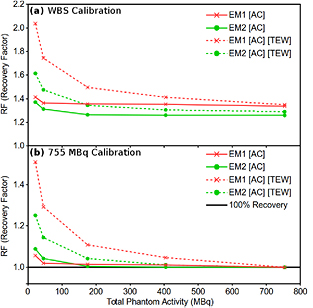
Figure 3. Whole image activity recovery factors (RF) for total reconstructed counts in the SPECT field-of-view for phantoms with activity in insert volumes only (No BG). Recovery factors (RF) are shown for EM1 (red) and EM2 (green) emission windows. The data are calibrated using the total reconstructed counts in (a) the WBS phantom data and (b) the highest activity scan 'No BG' cylindrical phantom scan (755 MBq).
Download figure:
Standard image High-resolution imageFigure 3(a) shows a clear overestimation of recovered activity ( ) at activities lower than 200 MBq when applying the TEW (dashed lines), to both calibration and object scans, in contrast to data with (AC) only (solid lines). The difference in activity recovery factor from 1.0 is improved for both (AC) and (AC)(TEW) when using calibration data with an identical geometry (figure 3(b)). However, there is still a significant overestimation of recovered activity when the TEW correction is applied at lower activities (<200 MBq), up to 51% and 25% for EM1 and EM2 respectively, (figure 3(b)).
3.1.2. CT guided VOI activity recovery.
The RF for  Lu calculated for a VOI corresponding to the 10 ml phantom inserts (outlined on co-registered CT data) is shown in figure 4. The SVS scan data (226 MBq) was used for calibration and provided separate calibration factors for scans with (AC)(TEW) and without the standard TEW correction (AC) applied. Data is presented for (a) 'No BG' phantom data and (b) 'BG' phantom data. Recovery factors are shown for both data sets (AC) (solid line) and (AC)(TEW) (dashed line) as a function of insert activity. For the 'BG' data the insert to phantom body activity concentration ratio is indicated by the line color,
  (green crosses),
  (pink circles), and
  (light blue squares).

Figure 4. Activity recovery factor (RF) for CT outlined volumes of interest (VOI) for (a) activity in insert volumes only (No BG) and (b) variable insert to phantom body activity concentration ratios (BG,  and
and  ) for EM1 (top) and EM2 (bottom) emission windows. RF is shown for data reconstructed with attenuation correction only ((AC)—solid line) and attenuation and TEW scatter correction ((AC)(TEW)—dashed line). SVS scan data (226 MBq, 10 ml insert) has been used for calibration.
Download figure:
Standard image High-resolution imageWith and without scatter correction applied, there is minimal difference in the values of RF for the 'No BG' data (figure 4(a)). For both the EM1 and EM2 photopeaks the activity recovery varies from 90% to 97% with decreasing activity. However, the addition of activity into the phantom body, figure 4(b), significantly changes the activity recovery in the CT defined VOIs. For the highest insert-to-background activity ratios ( ), the difference between recovered activity and known activity is 10% or less for EM1 and EM2 (blue lines) for both (AC) and (AC)(TEW) data. As the background activity increases relative to the insert activity the value of RF increases for both EM1 and EM2 (purple and green lines), up to a maximum of 1.8(3) (
 overestimation) and 1.4(2) (
 overestimation) for EM1 and EM2 respectively with (AC) only. When the TEW correction is applied the overestimated value of RF (for a
  insert-to-background activity ratio) is reduced to ∼1.2 (20%) for EM1 and EM2, with the largest reduction for EM1 (which has higher underlying scatter).
3.2. Monte Carlo simulation
3.2.1. Validation of Monte Carlo simulation.
Validation of simulated results by comparison to experimental measurements, is essential for all simulation techniques. Accurate validation is particularly important for MC simulation when using the output to provide insight into experimental phenomena which are not directly observable such as gamma ray tracking in a SPECT camera system. A comparison of the simulated (red line) and experimental (black line) energy spectrum from the Infinia-Hawkeye-4 PHA acquisition is shown in figure 5 for a water filled phantom with three 10 ml inserts containing  Lu, acquired using MEGP collimators. The true scattered component of the simulated
  Lu emission spectrum (TS) is also shown (blue dashed line). Figure 5 shows good agreement both in the photo-peak and lower energy Compton scattered regions for the complex emission from
  Lu. In addition the simulation correctly reproduces the emission and detection of Pb x-rays. The close agreement with experiment, across the whole energy spectrum (when the measured low energy detector efficiency and cut off are included), supports the choice of physics processes in the simulation and validates the global photon transport in our model.

Figure 5. Emission spectrum for a water filled phantom measured with an Infinia-Hawkeye-4 SPECT camera (black) and from Monte Carlo simulation (red) for  Lu with MEGP collimator. The true scattered (TS) component of the simulated spectrum (from MC simulation) is also shown (blue). The standard photopeak emission (EM) and adjacent scatter windows (SC) for the TEW correction are indicated by vertical lines.
Download figure:
Standard image High-resolution imageFigure 6 shows; (a) a representative projection of the experimental data from the 'No BG' scans (with  Lu) from the Infinia-Hawkeye SPECT camera and (b) the corresponding projection from our MC simulation. A horizontal profile through the inserts is shown (on both a linear and logarithmic scale) in figure 6(c) for the experimental (blue) and simulation (red dashed line). There is excellent agreement across the whole profile. The simulated 2D projection (figure 6(b)) closely reproduces that of the experiment with a peak-signal-to-noise ratio (PSNR) (Al-najjar and Soong 2012) of 71.2(1) dB for the two projection sets. Figure 6(d) shows the variation in total counts in each projection, corresponding to the head position for a tomographic acquisition. The variation in count rate, which depends on the specific source activity distribution and densities of the phantom and patient bed, is fully reproduced, further validating the geometry and material composition of our SPECT camera model for the full range of direct observables from a commercial SPECT camera.
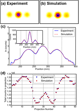
Figure 6. Projection of water filled phantom with three  Lu filled 10 ml inserts, (a) from Infinia-Hawkeye SPECT camera, (b) from Monte Carlo simulation. (c) Horizontal profile through the inserts for experimental (blue) and simulation (red dashed) data (insert shows linear scale). (d) Total counts in projection as a function of projection number, corresponding to the head position (0–360°, for a dual head tomographic SPECT acquisition.
Download figure:
Standard image High-resolution image3.2.2. Photopeak composition.
Table 3 shows the composition of events reconstructed within VOIs outlining the cylindrical inserts in the simulated 'BG' phantom data. Also shown is the corresponding event composition for the larger NEMA PET phantom data with 278 ml cylinder (described in section 2.3.2). The fraction of the total events detected in the EM1 and EM2 photopeak windows is classified according to the number of Compton interactions (scattered and unscattered) and the physical origin of the emitted photon (from phantom inserts or body). Data is presented for phantoms with variable insert to background activity ratios ( and
and  ) and also with no background activity (Calib). The largest contribution to the quoted uncertainty is due to iteratively reconstructing a subset of the total events detected in the photopeak. The fraction of events removed in each VOI by applying the standard TEW correction are also shown ('comparison with TEW correction'). For an ideal scatter correction this value should be equal to the total number of scattered events from the insert and body (shown as 'Total scattered events' in table 3). However, these data show an overestimation of scattered events when using the TEW. As an example, for the
  insert to body activity ratio data in the EM1 photopeak (column 5, table 3), the fraction of total scattered events (sum of 'insert scattered' + 'body scattered') is
  (
( ). In contrast for the same data the TEW correction estimates that 40% of the total events are scattered ('TEW correction'), an overestimation of 7%. A similar level of overestimation is seen with the TEW scatter correction with increased insert-to-background ratio and for the larger 278 ml insert data, with reduced scatter for the EM2 window.
Table 3. Composition of events in photopeak windows reconstructed within a VOI corresponding to cylindrical inserts for MC simulated SPECT data.
| Photopeak | Event Origin | Compton Scatter |
 ml inserts and body activity ml inserts and body activity |
278 ml insert and body activity | ||||||
|---|---|---|---|---|---|---|---|---|---|---|
| Insert to body activity ratio | Insert to body activity ratio | |||||||||
| Calib |
 |
 |
 |
Calib |  |
 |
 |
|||
| EM1 | Insert | Unscattered | 0.90(2) | 0.43(2) | 0.67(2) | 0.75(2) | 0.87(1) | 0.66(1) | 0.79(1) | 0.83(1) |
| EM1 | Body | Unscattered | 0.23(2) | 0.12(2) | 0.09(2) | 0.13(1) | 0.05(1) | 0.03(1) | ||
| EM1 | Insert | Scattered | 0.10(2) | 0.04(2) | 0.06(2) | 0.07(2) | 0.13(1) | 0.10(1) | 0.11(1) | 0.12(1) |
| EM1 | Body | Scattered | 0.29(2) | 0.15(2) | 0.08(2) | 0.11(1) | 0.04(1) | 0.02(1) | ||
| Total scattered events | 0.10(2) | 0.33(3) | 0.21(3) | 0.15(3) | 0.13(1) | 0.21(1) | 0.15(1) | 0.14(1) | ||
| Comparison with TEW correction |
0.16(2) | 0.40(2) | 0.28(2) | 0.21(2) | 0.27(1) | 0.36(1) | 0.29(1) | 0.28(1) | ||
| EM2 | Insert | Unscattered | 0.94(2) | 0.55(2) | 0.77(2) | 0.83(2) | 0.92(1) | 0.78(1) | 0.87(1) | 0.89(1) |
| EM2 | Body | Unscattered | 0.31(2) | 0.14(2) | 0.09(2) | 0.12(1) | 0.04(1) | 0.03(1) | ||
| EM2 | Insert | Scattered | 0.06(2) | 0.03(2) | 0.05(2) | 0.05(2) | 0.08(1) | 0.07(1) | 0.08(1) | 0.08(1) |
| EM2 | Body | Scattered | 0.10(2) | 0.05(2) | 0.03(2) | 0.03(1) | 0.01(1) | 0.01(1) | ||
| Total scattered events | 0.06(2) | 0.13(3) | 0.10(3) | 0.08(3) | 0.08(1) | 0.10(1) | 0.09(1) | 0.09(1) | ||
| Comparison with TEW correction |
0.10(2) | 0.21(2) | 0.15(2) | 0.12(2) | 0.16(1) | 0.17(1) | 0.14(1) | 0.14(1) | ||
aEvents classified by number of Compton interaction (Unscattered = 0, Scattered >0). bNo background activity. cFraction of events removed by TEW correction. Note: The fraction of total events detected in the VOI are given (standard uncertainties referred to the corresponding last digits of the quoted result are quoted in parentheses).
Figure 7 presents data from table 3 filtered by the 3D position of the origin of the event detected within the reconstructed regime. The fraction of total events originating from the phantom body background activity, detected within an VOI outlining the cylindrical inserts, is shown as a function of distance from the VOI (measured with 4.4 mm voxels). Data are shown for the EM1 and EM2 photopeaks for (a) 10 ml cylindrical insert (25 mm diameter) and (b) 278 ml cylindrical insert (44 mm diameter) with varying insert to background activity ratios. The contribution of unscattered background activity events (solid lines) and Compton scattered events (dashed lines) is also indicated. The different characteristics of these two event types is striking, the scattered events (dashed line) originate almost isotropically throughout the body of the phantom whilst the unscattered events (solid line) occur mainly in the voxels closest to the VOI and rapidly fall off with distance, suggesting these events are due to partial volume effects.
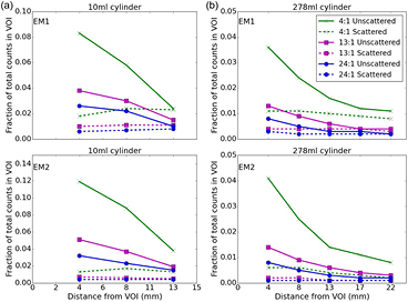
Figure 7. Origin of events from phantom body background activity detected in a VOI outlining (a) 10 ml cylindrical insert and (b) 278 ml cylindrical insert, from the MC simulated data. The contribution of unscattered background activity events due to partial volume effects (solid line) and Compton scattered events (dashed line) as a function of distance from the VOI is shown (The insert to background activity concentration ratio is indicated by line color).
Download figure:
Standard image High-resolution imageThe data presented in table 3 were used to calculate the contribution of scattered and unscattered events originating in the background to the change in activity recovery factor,  RF (table 4). The contribution from scattered photons is seen to be due to incorrect estimation of the true scatter when using the TEW correction, in both the calibration and object scans. The contribution of unscattered background events is a result of incomplete partial volume effect compensation. As an example, for the
  insert to body activity ratio data in the EM1 photopeak (column 3, table 4) the contribution of scattered photons will reduce the recovery activity by 11% (line 1) whilst the partial volume contribution overestimates the recovery by 53% (line 2), resulting in a total overestimation of activity by 42% (line 3). The relative contribution of partial volume events to
  RF for the larger 278 ml cylinder data is significantly reduced, as might be expected, in comparison to a smaller 10 ml cylinder.
Table 4. Total change in activity recovery factor (RF, no units) for MC simulated data with phantom background activity
| Photopeak |  ml inserts and body activity ml inserts and body activity |
278 ml insert and body activity | |||||
|---|---|---|---|---|---|---|---|
| Insert to body activity ratio | Insert to body activity ratio | ||||||
 |
 |
 |
 |
 |
 |
||
 RF from scattered photons RF from scattered photons |
EM1 | −0.11(2) | −0.06(2) | −0.03(2) | −0.08(1) | 0.00(1) | 0.00(1) |
 RF from PVE RF from PVE |
EM1 | 0.53(2) | 0.18(2) | 0.13(2) | 0.20(1) | 0.06(1) | 0.03(1) |
 RF Total RF Total |
EM1 | 0.42(3) | 0.12(3) | 0.10(3) | 0.12(1) | 0.06(1) | 0.03(1) |
 RF from scattered photons RF from scattered photons |
EM2 | −0.10(2) | −0.04(2) | −0.01(2) | −0.02(1) | 0.02(1) | 0.02(1) |
 RF from PVE RF from PVE |
EM2 | 0.56(2) | 0.18(2) | 0.10(2) | 0.16(1) | 0.05(1) | 0.03(1) |
 RF total RF total |
EM2 | 0.46(3) | 0.14(3) | 0.09(3) | 0.14(1) | 0.7(1) | 0.05(1) |
aFrom data presented in table 3. bDue to incorrect estimate of scatter from TEW correction. cDue to unscattered events originating in phantom body. Note: The table shows the contributions from scattered photons and partial volume events (standard uncertainties referred to the corresponding last digits of the quoted result are quoted in parentheses)a.
3.2.3. Localized energy spectra.
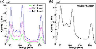
Simulated localized energy spectra for events detected in reconstructed VOIs outlining three 10 ml inserts, within a single phantom, with  and
and  insert to background ratios are shown in figure 8(a). The corresponding total phantom energy spectrum, as measured by clinical SPECT systems, is shown in figure 8(b). The peak-to-background ratio for the 113 and 208 keV photopeaks in figure 8(a) varies significantly with changes in background activity in contrast to the averaged total energy spectra from the sum of all three inserts which the SPECT camera records, shown in figure 8(b).
Figure 8. Simulated energy spectra for a phantom containing  Lu in three 10 ml inserts with
  and
and  insert to background activity ratios. (a) Spectrum of events detected in clinically reconstructed 10 ml VOIs. (b) Corresponding simulated whole phantom spectrum, as detected with a clinical SPECT system.
Download figure:
Standard image High-resolution image
4. Discussion
Accurate clinical MRT activity quantification requires a scatter correction technique which can be consistently applied across a range of activities and geometries, often occurring within the same image. An ideal correction should fully reproduce the scatter in all regions of a reconstructed image. The stability of a scatter correction method as a function of activity is particularly important at later imaging time points in MRT where clinical constraints set an upper limit on the length of a SPECT acquisition, resulting in reduced detection statistics for lower activities. Additional uncertainty can be introduced into a TAC measurement if the scatter correction does not accurately represent scattered photons for all time points in the imaging sequence.
4.1. Activity quantification
4.1.1. Whole image activity recovery.
Figure 3 demonstrates a significant overestimation in activity recovery for total counts in the SPECT field-of-view when a TEW scatter correction is applied at low activities ( 200 MBq total activity). These activities correspond to clinically observed total activities in the SPECT field-of-view for day 3 and day 6 NET patient
  Lu MRT imaging. In contrast the (AC) only data shows consistent activity recovery for an order of magnitude change in activity with an increase in RF of <10% below 200 MBq (see figures 3(a) and (b)). This overestimation of recovered activity when TEW correction is applied is present even when using an identical calibration scan, a best case scenario which is only possible with phantom data (see figure 3(b)).
As activity reduces in the phantom the total counts in the measured energy spectrum (figure 5) will be reduced, assuming a fixed acquisition duration. The integrated counts in the adjacent TEW scatter windows will reach zero much quicker than in the photopeak window as the activity is reduced. For low total activities the number of voxels where this condition is met, and hence no scatter correction occurs, will rise significantly. When this condition occurs the scatter window distribution no longer represents the background in the photopeak window and the TEW subtraction correction will no longer be valid. This leads to an overestimation of recovered activity when using a single calibration factor for all imaging time points, as observed in figure 3.
The large increase in activity recovery observed when applying the TEW at low activities, in contrast to using (AC) only, suggests that automatic application of a TEW scatter correction for whole image activity quantification should be undertaken with caution. This is of particularly clinical relevance when performing dosimetry using a single SPECT image in combination with a sequence of whole body scans.
4.1.2. CT guided VOI activity recovery.
When considering activity recovery for a CT defined VOI outlining a phantom insert containing activity (figure 4), it is typically the voxels with highest count rates within the image which are being considered. As a consequence the condition when the TEW no longer represents the scatter distribution (as previously discussed for whole image activity recovery), is unlikely to occur in the voxels within the VOI due to their higher number of statistics. Therefore, there is good activity recovery with the 'No BG' data for both the (AC) and (AC)(TEW) data using the SVS calibration factor. Figure 4(a) shows activity recovery factors ranging from 90–97% for both EM1 and EM2—analogous with the results seen for higher whole image activities, shown in figure 3. The value of RF provides a benchmark for the accuracy of activity recovery when using a relative calibration technique with calibration factors which correspond exactly to the volume being considered (calculated for a specific reconstruction protocol). The increase in RF with decreasing activity seen in figures 4(a) and (b) for both (AC) and (AC)(TEW) data is a result of the increased influence of noise at lower activities. For example, the noise level for the 'No BG' 250 MBq per insert scan (0.3%, measured using a VOI placed away from the insert) will correspond to a noise level of ∼9% in the lowest 7 MBq per insert scans. This is comparable to the 7(2)% increase in RF between the highest and lowest activity scans shown in figure 4(a).
The observed overestimation of activity recovery for a phantom insert with the introduction of background activity to a phantom may not be entirely unexpected. Exact activity localization can only be achieved with perfect compensation for scatter, partial volume and attenuation correction, whilst clinical SPECT imaging, by necessity, relies on approximate corrections. Whilst the TEW scatter correction provides improved values of RF, in comparison to using (AC) only, there is still a significant overestimation of recovered activity (see figure 4(b)). The underlying source of this overestimation is discussed in detail below in section 4.2.
4.2. Photopeak composition
It is clear from the distribution of phantom body background events shown in figure 7, and the data presented in table 3, that the composition of reconstructed photopeak events changes significantly with the introduction of activity in the phantom body. There are also significant differences between the 10 ml and larger 278 ml cylindrical insert data. For all data sets the TEW scatter correction overestimates the true total scatter ('Total scattered events' in table 3). The number of extra counts removed by the TEW however, varies significantly for each energy window and cylinder geometry. Therefore the use of a single calibration scan can only partially compensate for this over-subtraction. The different distributions of unscattered and scattered events from the background source as a function of the distance of the decay origin from the insert VOI (figure 7) is striking. The distribution of unscattered body events, which occur mainly in the voxels closest to the VOI, indicates that they are the result of partial volume effects which are not correctly compensated for. The magnitude of the partial volume effects, which is dependent on the choice of reconstruction parameters, is reduced when considering the larger 278 ml insert data (see table 4 and figure 7(b)). The data in figure 7 suggests that the majority of partial volume effects occur within the first 4 voxels from the insert. This is in agreement with the work of Shcherbinin et al (2012) who reported that for an Infinia Hawkeye camera with 4.4 mm voxels, expanding the VOI by four voxels encompassed the majority of activity spill-out from the VOI. This approach does not compensate for the contribution from the uniform distribution of scattered events (see figure 7).
The use of MC simulation has allowed the contributions of incomplete partial volume correction and TEW scatter correction to the total activity RF to be fully separated (table 4). For the data presented in this work applying a TEW correction can result in a change in RF from incorrect estimation of scattered photons of up to 11% for EM1 (10%, EM2) for a 10 ml cylinder with  insert to body activity ratio. This effect is reduced with increasing insert to body activity ratio and is also observed for the larger 278 ml data. The largest change in recovery factor (RF) in table 4, however, comes from unscattered events originating from the background source detected in the VOI due to partial volume effects. This results in additional recovered activity for all insert to body activity ratios in both geometries, with a maximum value over 50% (10 ml insert) and 20% (278 ml insert) in both emission windows. The partial volume effects contribute different amounts in the calibration and imaging scans and are therefore not fully compensated for with commercial clinical systems (Dewaraja et al 2012).
4.3. Suitability of TEW for accurate activity quantification
The results presented in this paper highlight the complex nature of SPECT activity quantification. Whilst we have demonstrated that good activity recovery is possible using a TEW correction with a relative calibration method, this is only possible when calibration and imaging conditions match exactly. The introduction of more clinically realistic conditions leads to a worsening in activity recovery. The simulated data presented in table 4 shows, by separating out the partial volume effects, that the TEW correction does not accurately represent scattered photons, even for large VOIs. Consequently even when using a relative calibration to compensate for any systematic error in scatter correction, for which identical phantom data represents the 'best case' scenario, the TEW can lead to significant errors in activity recovery.
It is clear from figure 8 that attempting to estimate the spatial distribution of scattered events by considering the distribution of scatter in the energy domain is inherently inaccurate. As previously discussed the peak-to-background ratio for both the 113 and 208 keV photopeaks in figure 8(a) varies significantly with changes in background activity, in contrast to the total phantom energy spectrum, as measured by clinical SPECT systems, shown in figure 8(b). Experimental measurements of localized energy spectra (as shown for simulated data in figure 8(a)) are not possible with clinical SPECT systems and hence any energy window based scatter correction will only reflect the average scatter distribution and can not fully reflect localized change in density and activity distribution.
A comparison of alternative approaches to energy window subtraction-based scatter correction for  Lu is given in de Nijs et al (2014). A CT based transmission-dependent scatter correction parameter method has been applied to quantification of
  Lu (Bailey et al 2015). However fully correcting a SPECT image for Compton scattered photons from a generalized activity concentration distribution is a highly complex problem which in reality can only be fully addressed using MC simulation. A generalized MC scatter correction method can be readily applied to determine the true scatter for any therapy or imaging isotopes. Ideally a quantitative scatter correction for MRT will be highly sensitive to the underlying patient specific activity distribution. Even a localized and optimized isotope-specific TEW correction cannot reflect a patient specific activity distribution without prior knowledge of the complete activity distribution. MC simulation has the potential to provide a corrected image with significantly reduced uncertainty in activity quantification. This will be addressed by a forthcoming article on a MC based approach to scatter correction, based on the True Scatter shown in figure 5, for
  Lu MRT.
5. Conclusion
The TEW scatter correction is commonly used to improve the image clarity of  Lu nuclear medicine data for clinical reporting (Ljungberg et al 2015). In this paper we have demonstrated that there can be a significant inaccuracy in activity quantification when using the TEW correction with
  Lu. Even with the relatively simple phantom activity distributions considered in this work the TEW scatter correction (using an appropriate relative calibration method) does not accurately compensate for scatter photons and can introduce additional errors in activity quantification. The change in activity recovery when using the TEW scatter correction is reduced for the EM2 energy window (which has a relatively lower scatter contribution). However, even for this 208 keV photopeak (which is often used clinically) careful consideration must be given to the choice of calibration applied at each imaging time point to avoid introducing additional errors in activity recovery. MC simulation has been used to perform a detailed analysis of the activity recovery for
  Lu MRT with SPECT, allowing the individual contribution of incomplete scatter correction and partial volume compensation to be separated. This has demonstrated that there can be a significant inaccuracy in activity quantification associated with any energy window based scatter correction. These energy windows based approaches only provide an approximation of the magnitude of scattered photons and are insensitive to localized variations in scatter. A new MC simulation based approach which provides accurate activity quantification input to dosimetry calculations for
  Lu is now essential.
Acknowledgments
This work was supported by the Science and Technology Facilities Council (ST/I006188/1 and ST/K002945/1).