

Abstract
This study compares 3D dose distributions obtained with voxel S values (VSVs) for soft tissue, calculated by several methods at their current state-of-the-art, varying the degree of image blurring. The methods were: 1) convolution of Dose Point Kernel (DPK) for water, using a scaling factor method; 2) an analytical model (AM), fitting the deposited energy as a function of the source-target distance; 3) a rescaling method (RSM) based on a set of high-resolution VSVs for each isotope; 4) local energy deposition (LED). VSVs calculated by direct Monte Carlo simulations were assumed as reference. Dose distributions were calculated considering spheroidal clusters with various sizes (251, 1237 and 4139 voxels of 3 mm size), uniformly filled with 131I, 177Lu, 188Re or 90Y. The activity distributions were blurred with Gaussian filters of various widths (6, 8 and 12 mm). Moreover, 3D-dosimetry was performed for 10 treatments with 90Y derivatives. Cumulative Dose Volume Histograms (cDVHs) were compared, studying the differences in D95%, D50% or Dmax (ΔD95%, ΔD50% and ΔDmax) and dose profiles.
For unblurred spheroidal clusters, ΔD95%, ΔD50% and ΔDmax were mostly within some percents, slightly higher for 177Lu with DPK (8%) and RSM (12%) and considerably higher for LED (ΔD95% up to 59%). Increasing the blurring, differences decreased and also LED yielded very similar results, but D95% and D50% underestimations between 30–60% and 15–50%, respectively (with respect to 3D-dosimetry with unblurred distributions), were evidenced. Also for clinical images (affected by blurring as well), cDVHs differences for most methods were within few percents, except for slightly higher differences with LED, and almost systematic for dose profiles with DPK (−1.2%), AM (−3.0%) and RSM (4.5%), whereas showed an oscillating trend with LED.
The major concern for 3D-dosimetry on clinical SPECT images is more strongly represented by image blurring than by differences among the VSVs calculation methods. For volume sizes about 2-fold the spatial resolution, D95% and D50% underestimations up to about 60 and 50% could result, so the usefulness of 3D-dosimetry is highly questionable for small tumors, unless adequate corrections for partial volume effects are adopted.
Export citation and abstract BibTeX RIS
1. Introduction
The continuous improvement and diffusion of hybrid SPECT-CT and PET-CT scanners has encouraged the calculation of (3D) dose distributions in targeted radionuclide therapy (TRT), using non-uniform activity distributions.
In the historical background of Monte Carlo (MC)-based internal dosimetry, the convolution of dose point-kernels (DPKs) with the 3D activity distribution was widely recommended when dealing with uniform media, as computationally more efficient than real-time MC calculations (Giap et al 1995, Kolbert et al 1997). DPKs for electrons and photons were calculated with MC codes and tabulated, introducing also analytical models to approximate dose-kernels and simplify the convolution algorithms (Leichner et al 1989, Prestwich et al 1989, Cross 1997). Subsequently, several groups updated the DPKs tabulations, comparing the results obtained with more recent MC codes (Janicki and Seuntjens 2004, Uusijärvi et al 2009, Botta et al 2011, Papadimitroulas et al 2012).
The voxel S values (VSVs) approach, introduced by the MIRD Committee (Bolch et al 1999), became more popular than DPKs, due to its recognized simplicity and reliability (Gardin et al 2003, Sarfaraz et al 2004, Dieudonné et al 2011, Ferrari et al 2012). In this approach, the average absorbed dose to the target voxel (t) can be calculated as:

where ÃS is the time-integrated activity in the source voxel (s) and St ← s is defined as:

where Δi is the mean energy emitted as radiation i per decay, φi is the absorbed fraction in t of the radiation i emitted in s and mt is the mass of the target voxel. VSVs must be calculated for each clinical setting, due to differences in reconstruction matrices, zoom factors (which involve changes in voxel size and/or shape) and absorbing medium. The differences among MC codes in the calculation of VSVs were studied afterwards, investigating also their impact on dosimetric calculations (Pacilio et al 2009). Recently, a freely available database of VSVs, calculated by direct MC simulations, was presented for seven radionuclides and thirteen voxel sizes in soft or bone tissues (Lanconelli et al 2012). To date, several strategies to calculate VSVs have been developed, exploiting direct MC computations (Strigari et al 2006, Pacilio et al 2009, Lanconelli et al 2012, Amato et al 2013a), convolution (Erdi et al 1998) or numerical integration of DPKs (Franquiz et al 2003). A method to calculate VSVs for a generic voxel size, by means of nuclide-specific fine-resolution VSVs (obtained with MC simulations) and a re-sampling procedure, was introduced by Dieudonné et al (2010). An analytical model for the calculation of VSVs for a generic electron and photon emission spectrum in cubic voxel sizes was proposed by Amato et al (2012). A rescaling method for obtaining VSVs for arbitrary voxel sizes based on fits, interpolations and re-samplings starting from nuclide-specific high-resolution VSVs was proposed by Fernández et al (2013).
Besides convolution techniques, direct MC simulation is considered the gold standard, since it accounts for inhomogeneity of absorbing media (Furhang et al 1997). Several studies pointed out the feasibility of real-time MC dosimetry (Sgouros and Kolbert 2002, Chiavassa et al 2006, Prideaux et al 2007, Hobbs et al 2009, Botta et al 2013, Marcatili et al 2013), the most remarkable of which presented the 3D-RD software (Prideaux et al 2007, Hobbs et al 2009). Despite the promising potentialities, MC-based treatment planning systems for TRT are not yet commercially available and the computational skills to implement them are not always present in clinical departments. So nowadays, the approach of convolution calculations by VSVs continues to play a role, at least for anatomic regions characterized by nearly-uniform density tissue (Dieudonné et al 2013).
The aim of this work is to compare the VSVs calculated by different currently available methods, studying the impact of the differences on 3D dose distributions. The methods employed have been previously validated by their proponents and were tested here at their state-of-the-art. So dose differences may derive from either methodology, or possible slight mismatches among input data for calculations (energy spectra, medium density and composition). Three methods are considered: 1. MC volume integration of DPKs (Cornejo Diaz et al 2006, Casacó et al 2008); 2. the analytical model presented by Amato et al (2012); 3. the rescaling method proposed by Fernández et al (2013). The local energy deposition (LED) hypothesis was also tested, assuming that all kinetic energy released from the emitted electrons is locally absorbed within the source voxel (Ljungberg and Sjögreen-Gleisner 2011, Chiesa et al 2012). The LED assumption may be useful to overcome the need of VSVs calculation and simplify dosimetric calculations for pure beta emitters, while the gamma emission, when present, must be accounted for by convolution. The VSVs obtained with direct MC simulations by Lanconelli et al (2012) were used as a reference. 3D dose distributions were compared in terms of cumulative Dose Volume Histograms (cDVHs) and dose profiles. Voxel-based models consisting of homogeneous spheroidal clusters of soft tissue were considered first, with uniform activity distribution of several radionuclides: 177Lu, 131I, 188Re and 90Y (188Re and 177Lu results are included in the supplementary data, (stacks.iop.org/PMB/60/051945) for reasons of space). The influence of typical spatial resolutions of real SPECT systems on dosimetric differences was also studied, blurring the activity distribution by Gaussian point spread functions (PSF) with various widths. Dosimetric differences were analysed also in clinical settings (non-uniform activity distributions) performing 3D dosimetry for patients treated with 90Y derivatives.
2. Materials and methods
2.1. Calculation of VSVs
2.1.1. Convolution of DPKs.
This method (Cornejo Diaz et al 2006) employs DPKs in water from the literature: the discrete DPKs published by Cross et al (Cross 1997, Cross et al 1992) for beta radiation, and the analytical functions of DPKs given by Furhang et al (1996) for gamma radiation. The discrete DPKs for beta radiation is fitted with empirical analytical functions, obtaining a maximum deviation with respect to the published values within 1.0% (Cornejo Diaz et al 2006). MC volume integration for each pair of source-target voxels is performed, obtaining the corresponding VSV, according to Franquiz et al (2003). Briefly, a given number (~106) of pairs of random points (one inside the source voxel, one in the target voxel) is simulated, and the corresponding absorbed dose rate is calculated for each distance between the two points. The St ← s for the pair of voxels is then obtained as the mean value of the absorbed doses from all couples of points. A correction is applied to the DPKs in water—based on the scaling factor method proposed by Cross et al (1992)—to calculate the S factors for the beta radiation in media other than water. The dose rate in the medium of interest (at a given distance r) is calculated from the dose rate in water as:

where ηW denotes the scaling factor, or relative attenuation of beta radiation for the considered medium compared to water, D(r) and DW(r) are the absorbed dose in the medium and water at the distance r and ρ, ρW are the densities of the medium and water, respectively. The methodology is implemented with a software developed in-house (Konvox, Borland Delphi 3 environment).
2.1.2. Analytical calculation method.
The analytical method for calculating VSVs, referred to a generic beta–gamma emitting radionuclide, was previously described (Amato et al 2012, Amato et al 2013b). It employs MC simulations with GEANT4 (Agostinelli et al 2003) of monoenergetic electrons and photons in voxelized regions of soft tissue with density 1.04 g cm−3 and composition from ICRP Publication 89 (Valentin 2003). The decay data from Stabin and da Luz (2002) were adopted. Cubic voxels with sizes between 3 and 10 mm (1 mm interval) and source energies in the range 10–2000 keV for electrons and 10–1000 keV for photons were used as input data. The average energy deposition per event (Edep) is represented as a function of the dimensionless 'normalized radius', defined as:

where l is the voxel side and R is the distance of the centre of the voxel (i, j, k) from the origin O, where the source voxel is centred. Regarding electrons, for each voxel side l and energy E, Edep(Rn) is fitted with the function:

whereas the fitting function for photons is:

a, b, c, r, s and f, g, h are parameters whose values depend on l and E. These parameters were previously reported as tabular data and for generic values of l and E they can be calculated by interpolation (Amato et al 2012). Then, the VSVs can be calculated as the quotients of energy deposition and voxel mass. For a generic beta–gamma emitting radionuclide, VSVs are obtained by a summation over all monoenergetic photon and electron emissions and an integration over the beta spectrum. A further generalization would allow also to obtain VSVs for different tissues, performing appropriate rescaling of the fitting parameters as a function of the tissue density (Amato et al 2013b).
2.1.3. Rescaling method.
The rescaling method (Fernández et al 2013) for obtaining VSVs for arbitrary voxel sizes between 1 and 10 mm starts from accurate sets of High Resolution (HR)-VSVs (one for electrons with 0.5 mm voxel size and one for photons with 1.0 mm voxel size) obtained for the radioisotope of interest by MC simulation (MCNPX v.2.7.a, Los Alamos National Laboratory, available at http://mcnpx.lanl.gov/). Simulations considered homogeneous soft tissue medium (density = 1.0 g cm−3) as defined by the National Institute of Standards and Technology website8, target-to-source voxel distances up to 10 cm, a uniform distribution of activity in the source voxel and all primary emitted radiations with their energy distributions and transition probabilities taken from the Eckerman and Endo tables (2008). The simulations were performed along a single line of voxels (on-axis HR-VSVs); interpolations within these values result in the HR-VSVs for voxels within a spherical volume. The rescaling of the HR-VSVs for obtaining VSVs for arbitrary voxel sizes (greater than or equal to 1.0 mm) is performed in two steps. (1) For integer voxel ratios (voxel ratio = new voxel size/voxel size from MC simulation), the deposited energies corresponding to the HR-VSVs data are resampled; (2) if the voxel ratio is not integer, an additional step of interpolation is carried out.
2.1.4. Local energy deposition.
The LED assumption allows calculating the beta contribution to the 3D dose distribution by multiplying the cumulated activity in the voxel for a unique dosimetric factor. The LED approach was initially reported by Bolch et al (1999) and assumes that all kinetic energy released from the beta emissions is locally absorbed within the source voxel (i.e. no charged particle escape). Consequently, for a continuous beta spectrum, the dosimetric factor is calculated as the quotient of the mean beta energy emitted per decay (Eβmean) and the mass of the voxel:

This calculation approach was recently adopted for voxel-based phantoms (Ljungberg and Sjögreen-Gleisner 2011) and clinical 3D dosimetry (Chiesa et al 2012). Recently, a new method based on LED was proposed, which rescales the dosimetric factor according to the mean absorbed dose to the target, accounting also for photon emissions (Traino et al 2013). The original LED calculation approach adopted in this study employs equation (7) to calculate the beta dosimetric factor, while for radionuclides also emitting photons, the result of a convolution calculation with VSVs for the emitted photons was added to the beta absorbed dose evaluated under the LED assumption. The VSVs for photon emissions used here were previously obtained (Pacilio et al 2009, Lanconelli et al 2012).
2.2. 3D dose distributions calculations
2.2.1. Voxel-based models.
The JAVA software program named CALDOSE (CALculations of DOse on Spheres and Ellipsoids) (Pacilio et al 2009) was used for dose convolution calculations, according to equation (1). CALDOSE allows 3D dose distribution calculations based on VSVs convolution on spheroidal or ellipsoidal clusters of cumulated activity. CALDOSE was modified to perform Gaussian filtering of the uniform activity distribution before the convolution calculation, simulating image blurring. Spatial resolutions in SPECT images may vary considerably (mainly, between 8–14 mm, as results from phantom studies), depending on general features of the SPECT system, image reconstruction methods, pre- and post-reconstruction filtering and radionuclide (Autret et al 2005, Gear et al 2007, Rault et al 2007, Seo et al 2010, Knoll et al 2012, Seret et al 2012, Kunikowska et al 2013 ). Three Gaussian PSFs with full-width-at-half-maximum (FWHM) of 6, 8 and 12 mm were chosen to blur absorbed dose distributions. Spheroidal clusters of soft tissue voxels (3 mm in size) with uniform activity distributions, having 251, 1237 and 4139 voxels (corresponding to radii of about 12, 20 and 30 mm respectively and masses of about 7, 35 and 116 g considering a density of 1.04 g cm−3) were simulated. The considered radionuclides were 131I, 177Lu, 188Re and 90Y, assuming always an activity concentration of 30 kBq per voxel. The VSVs calculated by Lanconelli et al (2012) were assumed as a reference, obtained for soft tissue (physical density 1.04 g cm−3, elemental composition as defined by Cristy and Eckerman (1987), decay spectra from Stabin and da Luz (2002)). Moreover, the VSVs reported by the MIRD Committee (Bolch et al 1999, available for 90Y and 131I) were also used for comparison. Diametral dose profiles and cDVHs were calculated for each case, reporting some examples. The cDVH is the integral of the differential DVH from D to Dmax (the maximum value of the absorbed dose to the irradiated volume). A systematic analysis of dosimetric differences in terms of D95%, D50% (i.e. the minimum value of the absorbed dose to 95% or 50% of the irradiated volume, respectively) and Dmax was reported.
2.2.2. Clinical cases.
Ten patients undergoing a 99mTc-MAA (macroaggregated albumin) dosimetry study as a surrogate of 90Y-resin-microspheres radioembolization were analysed to apply the different VSVs in a clinical setting. After the injection of about 74 MBq of 99mTc-MAA into the hepatic artery, patients underwent a SPECT/CT scan to assess the activity distribution in the liver. All images were acquired with a dual-head gamma camera (Infinia II—GE Healthcare, Waukesha, WI) using a LEHR collimator and setting 60 projections, matrix 128 × 128 (4.42 mm voxel size), 30 s per view; double energy window acquisition: 140 keV ± 20% for emissive image and 112 keV ± 5% scatter image window, automatic body contour. To perform attenuation correction, a low dose CT scan was also acquired (120 kV, automatic tube current modulation with Noise Index <25). AW-Server 2.0 (GE Healthcare) was used to coregister rigidly SPECT and CT images, using as landmarks 3 radioactive-opaque markers positioned on the patient skin (one at the sternum level and 2 at hip level) before CT and SPECT acquisitions. Iterative reconstruction of SPECT images was performed using the standard protocol of Xeleris 3.1 workstation (GE Helthcare), with the OSEM algorithm (8 iterations, 6 subsets, no post-reconstruction filtering), including attenuation and scatter corrections. The tomographic spatial resolution was about 13 mm (as results from phantom studies, i.e. with a line source having an inner diameter of 1 mm and about 150 MBq cm−1 of 99mTc, inserted centrally into the tank of a Carlson Phantom, parallel to its longitudinal axis). Microspheres are not metabolized but remain trapped permanently in the liver so 90Y physical decay was considered to assess the biokinetics (Chiesa et al 2011, Walrand et al 2014). The hypothesis that 99mTc-MAA describes the 90Y microsphere distribution was assumed, meaning that in each voxel the activity of 90Y microspheres is directly proportional to the voxel count in 99mTc-SPECT. A relative calibration was applied to convert the SPECT images into an activity map, by dividing the total number of counts in the whole liver region by the total injected activity (Dieudonné et al 2011, Chiesa et al 2012). For the purpose of this study, we assumed that all patients were injected with 1 GBq of 90Y and that the target region of each patient was defined as the iso-count level of 50% of the maximum value. The 3D absorbed dose distributions for the different VSVs tables were calculated by convolving the 3D cumulated activity map with the corresponding VSVs matrix using MATLAB version 7.9.0.529 (R2009b). Again, the results obtained with the VSVs calculated by Lanconelli et al (2012) were used as reference. Comparisons were performed in terms of dose profiles and cDVHs. The differences (mean value and range of variation), in terms of D95%, D50%, Dmax, between the results obtained with each tested method and those derived with the reference VSVs, were reported for all patients.
3. Results
3.1. Direct comparison between VSVs data sets
The comparison between the VSVs data sets for a voxel size of 3 mm is shown in figure 1 for 90Y and 131I. The methods described in sections 2.1.1, 2.1.2, 2.1.3 and 2.1.4 are hereinafter denoted as 'Konvox', 'AM', 'Rescaling' and 'LED', respectively. The reference VSVs are denoted as 'Reference data', whereas those from Bolch et al (1999) as 'MIRD' (reported when available). Figure 1 shows the relative percent differences for all VSVs datasets, with respect to the reference data, as a function of the normalized source-target distance (equation (4)). 90Y VSVs are in good agreement up to about Rn = 2. A systematic underestimation (AM) and overestimation (Rescaling) of VSVs can be observed in the 'transition region' (i.e. the region where the energy deposited by bremsstrahlung and/or primary photons begins to prevail on the energy deposited by beta rays, Rn range of 2–4). At larger distances (beyond Rn = 4.5, where the bremsstrahlung contribution prevails), Rescaling gives accurate results up to Rn = 5, whereas AM gives moderate differences (±10%). Konvox remains in agreement with the reference data up to about Rn = 3.5, then values reduce rapidly to zero, because the DPKs of Cross et al (1992) do not account for the bremsstrahlung contribution beyond the maximum CSDA range. Differences for MIRD data are notably larger, from about Rn = 3. For 131I, Konvox results are virtually coincident with the reference data; Rescaling gives a good agreement beyond the transition region, whereas at short distances (Rn ≤ 1.4), differences are up to about 8%; AM presents appreciable differences, either in the transition region, or beyond (±13%). MIRD data show major deviation in the transition region and large statistical fluctuations beyond it. For 90Y and voxel size of 4.42 mm (of interest for the clinical cases considered here), the trend of VSVs difference is almost the same for all methods (data not reported), except for AM, which shows differences of opposite sign for the first neighbors, with respect to the 3 mm voxel size.
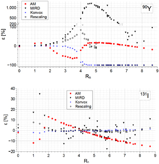
Figure 1. Comparison between the VSVs obtained with several methods, for a voxel size of 3 mm. The panels report the relative percent differences for VSVs with respect to the reference data, as a function of the source-target normalized distance, for 90Y (top) and 131I (bottom).
Download figure:
Standard image High-resolution imageTable 1 reports the percent differences associated with the voxel S factors S0 0 0, S0 0 1, S0 1 1, S1 1 1, with respect to the reference data. The first two columns refer to a voxel size of 3 mm, whereas the differences associated to 90Y and voxel size of 4.42 mm are reported in the last column.
Table 1. Percent differences for the VSVs S0 0 0, S0 0 1, S0 1 1, S1 1 1, with respect to the reference dataset, for the three methods tested here with 90Y and 131I. The first two columns are referred to a voxel size of 3 mm, whereas the differences associated to 90Y and a voxel size of 4.42 mm are reported in the last column.
| Method | i,j,k | 90Y | 131I | 90Y |
|---|---|---|---|---|
| AM | 0,0,0 | −2.5 | −2.0 | −0.5 |
| 0,0,1 | 13.8 | −11.9 | −0.9 | |
| 0,1,1 | 15.8 | −8.3 | −6.4 | |
| 1,1,1 | 1.4 | 2.8 | −22.6 | |
| Konvox | 0,0,0 | −1.9 | −0.8 | −1.8 |
| 0,0,1 | −1.1 | −2.0 | −0.8 | |
| 0,1,1 | −0.2 | −2.5 | −0.4 | |
| 1,1,1 | 0.2 | −1.2 | −0.6 | |
| Rescaling | 0,0,0 | 3.1 | 5.7 | 2.9 |
| 0,0,1 | 3.3 | 7.6 | 4.2 | |
| 0,1,1 | 4.8 | 6.6 | 7.2 | |
| 1,1,1 | 7.2 | 2.1 | 11.0 |
(*)Percent differences associated to a voxel size of 4.42 mm.
Analogous comparisons for 188Re and 177Lu are reported in the supplementary material (figure 1s and table 1s) (stacks.iop.org/PMB/60/051945).
3.2. Comparison among 3D absorbed dose distributions
3.2.1. Voxel-based models.
cDVHs and dose profiles referred to 90Y and the smallest spheroidal cluster (251 voxels) with the unblurred activity distribution are reported in figure 2. For dose profiles, the absorbed dose was normalized with respect to the total cumulated activity in the cluster, assuming physical decay.

Figure 2. Comparison between cDVHs (a) and dose profiles (b) for the smallest spheroidal cluster (251 voxels) uniformly filled with 90Y and unblurred activity distribution. For dose profiles, the absorbed dose was normalized with respect to total cumulated activity in the cluster, calculated assuming physical decay.
Download figure:
Standard image High-resolution imageFigure 3 reports the results for 90Y and 131I in the largest spheroidal cluster (4139 voxels) with unblurred activity distribution. For 90Y, the diametral absorbed dose profiles (figure 3(b)) confirm the differences observed by cDVHs data (figure 3(a)). The mean beta energy considered for LED was derived from the beta spectrum used in the calculations of the reference VSVs, so the absorbed dose to voxel obtained with LED is always equal to or greater than the Dmax value obtained by convolution of the reference data.

Figure 3. Comparison between cDVHs and dose profiles for the greatest spheroidal cluster (4139 voxels) and unblurred activity distribution, for 90Y (a) and (b) and 131I (c) and (d). For dose profiles, the absorbed dose was normalized with respect to total cumulated activity in the cluster, calculated assuming physical decay.
Download figure:
Standard image High-resolution imageAlso for 131I (figures 3(c)–(d)), some differences among cDVHs are present and similar to those observed for 90Y. In this case for the LED method, the absorbed dose contribution obtained by convolution of gamma VSVs was added to that deriving from LED for beta, so cDVHs and dose profiles are no longer represented by a step function and a constant value, respectively.
Table 2 reports the difference for the three dosimetric indicators (ΔD95%, ΔD50% and ΔDmax from the cDVHs) associated to the three clusters studied here, for 90Y and 131I. Analogously, data for 188Re and 177Lu are reported in the supplementary material (stacks.iop.org/PMB/60/051945) (table 2s).
Table 2. Percent differences of the dosimetric indicators from the cDVHs (D95%, D50% and Dmax) of the clusters examined here (voxel size of 3 mm), obtained with the various methods and unblurred activity distributions, with respect to the results obtained with the reference VSVs, for 90Y and 131I.
| Method | Cluster of 251 voxels | Cluster of 1237 voxels | Cluster of 4139 voxels | |||||||
|---|---|---|---|---|---|---|---|---|---|---|
| Radionuclide | ΔD95% (%) | ΔD50% (%) | ΔDmax (%) | ΔD95% (%) | ΔD50% (%) | ΔDmax (%) | ΔD95% (%) | ΔD50% (%) | ΔDmax (%) | |
| AM | 90Y | 3.0 | 4.7 | 3.7 | 1.5 | 3.9 | 3.7 | 2.8 | 4.1 | 3.7 |
| 131I | −3.2 | −3.2 | −3.3 | −2.3 | −3.3 | −3.4 | −3.1 | −3.4 | −3.4 | |
| Konvox | 90Y | −1.5 | −1.2 | −1.0 | −1.5 | −1.0 | −1.0 | −1.4 | −0.9 | −1.0 |
| 131I | −1.5 | −1.5 | −1.0 | −0.2 | −1.2 | −1.0 | −1.5 | −1.0 | −1.0 | |
| Rescaling | 90Y | 4.5 | 4.7 | 5.3 | 4.4 | 4.4 | 5.2 | 4.6 | 5.1 | 5.3 |
| 131I | 4.9 | 5.8 | 5.9 | 6.2 | 5.3 | 5.1 | 5.1 | 5.6 | 5.2 | |
| LED | 90Y | 58.5 | 25.6 | 0.0 | 56.2 | 5.1 | 0.0 | 50.2 | 0.9 | 0.0 |
| 131I | 7.9 | 2.3 | 0.2 | 8.9 | −0.3 | −0.2 | 7.8 | −0.2 | −0.2 | |
| 131I |
3.7 | −3.4 | −3.6 | 3.0 | −8.2 | −11.8 | 1.3 | −9.7 | −12.4 | |
(*)Percent differences for 131I with the LED assumption, without the contribution of gamma emissions.
For AM, the differences are consistent with those observed for the corresponding VSVs and within about 5%. The oscillating trend from negative to positive values (from one radionuclide to another) is due to the calculation of VSVs by fitting functions, which can yield values sometimes higher, sometimes lower than those obtained for monoenergetic sources, from which the fitting functions were determined. The highest differences were observed for 90Y, probably because the methodology is implemented for electrons energy up to 2 MeV, whereas 90Y beta emissions have energy up to about 2.2 MeV, thus needing an extrapolation above 2 MeV. For Konvox, a negative difference seems systematic for most of the dosimetric indicators. This is consistent with the underestimation of the VSVs for small source-target distances (with respect to the reference dataset), reported in table 1. The differences are limited for all radionuclides, except for 177Lu (see supplementary data) (stacks.iop.org/PMB/60/051945), for which slight differences in the beta spectrum energy sampling may play a role. The approach used by Cross et al (1992) to consider the singularity of DPK functions at r = 0 could be also important, mainly for 177Lu having relatively low beta energies, as pointed by Janicki and Seuntjens (2004). As regards rescaling, the VSVs calculations are referred to soft tissue with unit density, differently from that used for the reference VSVs (1.04 g cm−3). The results in tables 1 and 2 seem coherent with this density difference. Also in this case, slight differences in beta spectrum energy sampling may contribute. For 177Lu, the differences are higher than other radionuclides (see supplementary data) (stacks.iop.org/PMB/60/051945), probably because 177Lu has beta emissions with the lowest energy, so the density difference has a higher influence on the absorbed dose. For LED, the percent differences are obviously related to the amount of lateral electron disequilibrium (i.e.particles escaping from the cluster, not balanced by particles entering from outside). For a given size of the cluster, it is expected that the higher the beta energy, the greater the electron disequilibrium effect, as evidenced by the corresponding increase in ΔD95% and ΔD50%. For a given radionuclide, the larger the cluster size, the lower the difference between the cDVH and a step function, so ΔD95% and ΔD50% decrease. The differences obtained for 131I without considering the gamma contribution (i.e. assuming only LED for betas) evidence that the gamma contribution on the absorbed dose increases with mass, while neglecting it differences down to about −10% for D50% and Dmax for the largest clusters arise.
Figure 4 shows the results for 90Y and 131I in the largest spheroidal cluster (4139 voxels) after blurring the activity distribution with a Gaussian PSF having a FWHM of 12 mm. The most evident outcome is the substantial agreement of LED with the other methods.
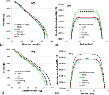
Figure 4. Comparison between cDVHs and dose profiles for the greatest spheroidal cluster (4139 voxels), for 90Y (a) and (b) and 131I (c) and (d), after blurring the activity distribution with a PSF having a FWHM of 12 mm. For dose profiles, the absorbed dose was normalized with respect to total cumulated activity in the cluster, calculated assuming physical decay.
Download figure:
Standard image High-resolution imageTo study the differences among methods for various degrees of image blurring and cluster sizes, ΔD95%, ΔD50% and ΔDmax have been calculated for PSFs with FWHM of 6, 8 and 12 mm, for the smallest and the largest clusters. The 3D dose distributions obtained with the reference VSVs for the unblurred activity distribution can be considered as the dosimetric 'gold standard', since the dose calculations obtained by convolution in medium with uniform density must correspond, in principle, to direct MC simulations (Dieudonné et al 2010, Dieudonné et al 2013). Figure 5 reports ΔD95% and ΔD50% for 90Y, as a function of the PSF FWHM, for the smallest (figures 5(a) and (b)) and the largest (figures 5(c) and (d)) cluster.

Figure 5. ΔD95% and ΔD50% for 90Y, as a function of the PSF FWHM, for the smallest (a)–(b) and the largest (c)–(d) cluster. The data denoted as 'MC' correspond to the differences between dosimetric calculations on the blurred and unblurred distributions, both performed with the reference VSVs calculated by direct MC simulations (Lanconelli et al 2012).
Download figure:
Standard image High-resolution imageThe data denoted as 'MC' correspond to the differences between dosimetric calculations on blurred and unblurred distributions, both performed with the reference VSVs. Figure 6 reports the ΔD95% and ΔD50% for 131I, as a function of the PSF FWHM, for the smallest (figures 6(a) and (b)) and the largest (figures 6(c) and (d)) cluster. Analogously, corresponding data for 188Re and 177Lu are reported in the supplementary material (stacks.iop.org/PMB/60/051945) (figures 2(s)–3(s)).
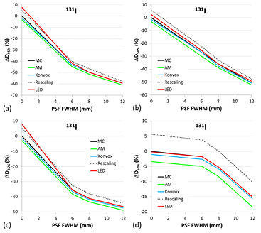
Figure 6. ΔD95% and ΔD50% for 131I, as a function of the PSF FWHM, for the smallest (a)–(b) and the largest (c)–(d) cluster. The data denoted as 'MC' correspond to the differences between dosimetric calculations on the blurred and unblurred distributions, both performed with the reference VSVs calculated by direct MC simulations (Lanconelli et al 2012).
Download figure:
Standard image High-resolution image3.2.2. Clinical cases.
All patients examined showed very similar trends of dosimetric results, so cDVHs and dose profiles were reported just for one patient, as an example. Figure 7 reports: (a) dose image (transaxial slice) obtained with the reference VSVs and the position for dose profile sampling, (b) cDVHs for a VOI (volume of interest) defined by an iso-count level of 50% (with respect to the maximum count value), (c) the dose profiles for several VSVs tables and (d) the percent differences for the dose profiles, with respect to the results obtained with the reference VSVs.

Figure 7. Dosimetric results obtained for a patient undergone to SIRT therapy: (a) dose image obtained with the reference VSVs and the segment where the dose profile was sampled, (b) cDVHs obtained with several VSVs tables, for a VOI defined by the 50% iso-count curve (with respect to the maximum count value), (c) dose profiles for several VSVs tables and (d) percent differences for the dose profiles (with respect to the results obtained with the reference VSVs).
Download figure:
Standard image High-resolution image
The uptaking VOIs resulted in the range 8–56 cm3. Reference 3D dose distributions (deriving from unblurred activity distributions) are not available in these cases, so the comparison was performed with respect to the dosimetric results obtained with the reference VSVs on the same images, even though they cannot represent reference dose distributions. Table 3 reports the mean difference and the corresponding variation range, for dosimetric indicators (with respect to the results obtained with the reference VSVs) for all treated patients. Outcomes for the large cluster, with a blurred activity distribution (FWHM = 12 mm), are also reported in the last three columns for comparison.
Table 3. Mean value and range of dosimetric indicators difference associated to each calculation method, with respect to the dosimetric results obtained with the reference VSVs, for all treated patients. For comparison, ΔD95%, ΔD50%, ΔDmax obtained for the large cluster with a blurred activity distribution (FWHM = 12 mm) are also reported in the last three columns.
| Method | Patients | Large cluster | ||||
|---|---|---|---|---|---|---|
| ΔD95% mean (range) (%) | ΔD50% mean (range) (%) | ΔDmax mean (range) (%) | ΔD95% (%) | ΔD50% (%) | ΔDmax (%) | |
| AM | −2.8 (−3.0/ − 2.6) | −3.0 (−3.2/ − 2.8) | −2.8 (−2.9/ − 2.4) | 4.0 | 3.9 | 3.7 |
| Konvox | −1.3 (−1.6/ − 0.7) | −1.3 (−1.7/ − 1.1) | −1.2 (−1.3/ − 1.2) | −2.0 | −1.0 | −1.0 |
| Rescaling | 4.3 (3.8/4.9) | 4.4 (4.1/4.7) | 4.4 (4.2/4.5) | 4.3 | 5.1 | 5.2 |
| LED | 7.9 (3.6/15.7) | 5.6 (2.8/9.5) | 12.8 (5.4/30.5) | 2.3 | 2.2 | 0.0 |
4. Discussion
4.1. Direct comparison among VSVs data sets
The most evident differences among the various methods are observed in the transition region, or beyond the maximum continuous-slowing-down-approximation range (where the energy is deposited solely by bremsstrahlung and/or primary gamma rays). Noteworthy, the dosimetric differences in the 3D dose distributions are mainly due to the VSVs referred to self-irradiation (i.e. S0 0 0) and first neighbors target voxels (Pacilio et al 2009, Lanconelli et al 2012).
4.2. Dose distributions with voxel-based models
When considering a perfect spatial resolution, the LED assumption with a uniform activity distribution yields a uniform absorbed dose distribution within the target, so the corresponding cDVH is a step function. On the other hand, convolution calculations evidence the effects of lateral electron disequilibrium. This effect is maximized when the smallest cluster and the most energetic beta emitter are considered (see figure 2). The DPKs convolution has proved an excellent trade-off among methods, with a good accuracy which could be further improved provided that updated DPKs are used.
When the image blurring is considered, differences between the cDVHs obtained by the several methods (above all, for LED) tend to decrease. The differences in the high dose region of the cDVHs (see figures 4(a) and (c)), represented by the central voxels of the cluster, remain essentially unchanged, as also evidenced by the dose differences in the central region of dose profiles (figures 4(b) and (d)). On the contrary, the absorbed dose in voxels near the edges decreases sharply, producing a strong decrease of D95% and D50% and masking the differences among the methods.
Generally, image blurring causes a strong decrease of the dosimetric indicators, regardless of the method used, as evidenced in figures 5 and 6 (as well as in figures 2(s) and 3(s) of the supplementary material) (stacks.iop.org/PMB/60/051945). For example, for 90Y and the smallest cluster (24 mm diameter), D95% decreases at about −45% with respect to the reference value and as expected, this decrease is less severe when the cluster size increases (about −30% for the largest cluster). Also for LED, D95% decreases strongly when increasing the blurring effects, until becoming comparable with the other methods. This is because the blurring of the true activity distribution by the PSF spreads the dose out more than convolution with the VSVs kernels. For ΔD50% and the smallest cluster (figures 5(b) and 6(b)), the general trend is similar to ΔD95%, whereas for the largest cluster (figures 5(c) and 6(c)), ΔD50% varies less abruptly with increasing FWHM, for all methods and radionuclides (see also figures 2(s) and 3(s) in the supplementary material) (stacks.iop.org/PMB/60/051945). As regards ΔDmax (data not reported), the trend generally observed for all radionuclides showed, for the smallest cluster, a decrease with FWHM increasing (starting from a FWHM of 6 mm), whereas for the largest cluster, ΔDmax remains constant after Gaussian filtering (whichever FWHM value).
In summary, LED yields a 3D dose distribution more and more similar with increasing of the blurring, until it becomes almost equivalent to that obtained with VSVs convolution, at typical spatial resolutions of clinical SPECT images. At the same time, blurring effects reduce slightly also the differences among the methods for VSVs calculations.
The data trend due to partial volume effects presented here is not surprising, however the impact that the limited spatial resolution of the SPECT images has on the dose map calculation is too often disregarded in dosimetric analyses. Actually, the spatial resolution of SPECT images is the main limiting factor for accurate dosimetry in small structures, nevertheless, the recent publications studying extensively these issues are few (Ljungberg and Sjögreen-Gleisner 2011, Pasciak et al 2014).
In the present work, an extensive analysis of the influence of SPECT image blurring in dosimetric assessments is also proposed. The severe degradation of cDVHs due to image blurring here observed is in good agreement with the data reported by Ljungberg and Sjögreen-Gleisner (2011) for tumour dosimetry, even though several differences are present between the two studying methodologies. In that previous publication, data are referred to a greater voxel size (6.5 mm) and cDVHs were obtained from MC simulations of experimental images, so involving the reconstruction process. In the present work, a 3 mm voxel size was considered and the tomographic reconstruction was not involved, focusing on voxel-based models. The method of tomographic reconstruction of experimental images could introduce further influences on the dose maps (e.g. the noise, above all when using a large number of iterations in an iterative MLEM/OSEM algorithm, or ringing artifacts when using the collimator-response correction) which would require additional, dedicated studies (Cheng et al 2013). The study by Pasciak et al (2014) presented an extensive analysis of the blur impact on dosimetry, but focused just on 90Y, whereas the data here presented are referred to several radionuclides. For 90Y, a general agreement can be noted also with that previous work, even though a direct comparison is not easy, due to differences in the dosimetric indicators: integral DVHs (i.e. the integral of the differential DVH from 0 to a given dose value) and related range of error (associated to the entire dose interval) in Pasciak et al (2014), cDVHs and associated ΔD95%, ΔD50% and ΔDmax in this work.
Today current interests in TRT are: correlation between tumor response and dosimetric indicators such as EUBED (whose calculation is based on the differential DVH), D90% or D70%; combination of TRT and external radiation therapy, which requires accurate 3D dosimetry to avoid toxicity and increase efficacy (Hobbs et al 2011, Ferrari et al 2012, Fourkal et al 2013, Grimes et al 2013, Cremonesi et al 2014). Blurring effects could severely affect the accuracy of activity distributions used as inputs to 3D dosimetry. Even for relatively 'large' VOI (i.e. 5-fold the spatial resolution), dosimetric indicators, derived from cDVHs and associated with high percentages of irradiated volume, could be considerably influenced by partial volume effects.
4.3. Clinical cases
All cDVHs showed a very similar shape and the differences among them are limited. The comparisons among dose profiles evidenced limited differences, having a nearly constant trend for the AM, Konvox and Rescaling, whereas LED shows an oscillating trend and could reach differences higher than 20–30%.
For the AM, limited differences of the dosimetric indicators are always negative, as also confirmed by dose profiles (see figure 7(d)), differently from the largest spheroidal cluster (always positive for 90Y, see table 3). This is due to the peculiarity of the method: for clinical cases, the voxel size (4.42 mm) differs from voxel-based models (3 mm). Since the VSVs are calculated with a new fit function, the sign of the dosimetric differences can change. Indeed, most of the differences associated to the VSVs reported in table 1 have an opposite sign for a voxel size of 4.42 mm, with respect to 3 mm. As regards Konvox and Rescaling, the differences of the dosimetric indicators are very similar to those obtained for 90Y in spheroidal clusters. So, the differences among calculation methods of VSVs are negligible also for clinical cases and the clinical condition of non-uniform activity distributions does not substantially change the differences among methods obtained with a blurred (uniform) activity distribution in a spheroidal cluster (except for the sign change of AM, due to the change in voxel size). As regards LED, differences are still limited, but considerably higher than others and also higher than the corresponding values obtained with voxel-based models, probably due to the influences of the non-uniformity in the activity distribution. The differences' trend is in substantial agreement with the work of Pasciak et al (2014), where it was postulated that the blur introduced by the scanner PSF combined with DPK convolution would result in over-estimation of the distribution of beta energy deposition away from the site of decay. Unfortunately, the reference dose distribution is unknown in clinical cases, so it is not possible to assess the most accurate methodology.
5. Conclusion
All methods here considered for VSVs calculation yield similar dosimetric results on voxel-based models with unblurred activity distributions, with differences limited or easily explainable. On the contrary, LED is not suitable in voxel-based models with unblurred activity distribution, or with imaging systems with high resolving power. The dosimetric differences decrease after blurring the activity distribution with Gaussian filters of increasing width, representing the limited spatial resolution of clinical SPECT images. The method of convolution of DPKs represents an advantageous strategy for calculation of VSVs, ensuring adequate accuracy without need of direct MC simulations. With blurring typically representative of the finite spatial resolution of clinical SPECT systems, LED has proved a useful trade-off, between ease of use and accuracy, to perform 3D dosimetry, even though in clinical cases dose differences with respect to reference data resulted higher than those of other methods. Partial volume effects effectively smooth results and reduce differences between methods, however they introduce errors in all methods compared to the true dose distribution. Partial volume effects of clinical SPECT images resulted the main concern for dosimetric accuracy. Considering that underestimation up to about 60% for D95% (or similarly D90%) and 50% for D50% could result for volumes of size about 2-fold the SPECT spatial resolution, the utility of 3D dosimetry could be highly questionable for small tumors, unless an adequate correction strategy for partial volume effects is adopted. Even for relatively 'large' VOIs (5-fold the spatial resolution), partial volume effects could influence considerably dosimetric indicators associated with high percentages of irradiated volume in cDVHs.
Footnotes
- 8
Available at http://physics.nist.gov/cgi-bin/Star/compos.pl?matno=261.