
Abstract
Magnetic particle imaging is a new approach to visualizing magnetic nanoparticles. It is capable of 3D real-time in vivo imaging of particles injected into the blood stream and is a candidate for medical imaging applications. To date, only one particle type has been imaged at a time, however, the ability to separate signals acquired simultaneously from different particle types or from particles in different environments would substantially increase the scope of the method. Different colors could be assigned to different signal sources to allow for visualization in a single image. Successful signal separation has been reported in spectroscopic experiments, but it was unclear how well separation would work in conjunction with spatial encoding in an imaging experiment. This work presents experimental evidence of the separability of signals from different particle types and aggregation states (fluid versus powder) using a 'multi-color' reconstruction approach. Several mechanisms are discussed that may form the basis for successful signal separation.
Export citation and abstract BibTeX RIS

Content from this work may be used under the terms of the Creative Commons Attribution 3.0 licence. Any further distribution of this work must maintain attribution to the author(s) and the title of the work, journal citation and DOI.
For more information on this article, see medicalphysicsweb.org
1. Introduction
Several medical imaging modalities can discriminate different signal origins or paths by detecting signals at different frequencies. For instance, magnetic resonance imaging (MRI) can spectrally separate signals from water and fat protons, because their chemical environment leads to different shifts of the resonance frequency (Dixon 1984). MRI can furthermore discriminate different nuclei by their intrinsically different resonance frequency at a given applied field strength, i.e. their different gyromagnetic ratio. This can, for instance, be used for synchronous imaging of anatomy (proton image) and functional fluorine markers (19F) (Keupp et al 2011). In computed tomography (CT), developments such as dual-energy CT (Alvarez and Macovski 1976) and spectral CT (Riederer and Mistretta 1977, Schlomka et al 2008) also aim to generate a material-dependent contrast based on energy resolved detection. In single photon emission computed tomography (SPECT), improvements in energy-resolved detectors enable multi-isotope imaging which is able to discriminate between the emissions from different radioactive tracer materials (Wagenaar et al 2006). Generally, in an attempt to maximize the diagnostic information obtained in a clinical imaging exam, the ability to acquire information in parallel at different energies becomes increasingly important.
Magnetic particle imaging (MPI) is a new imaging approach (Gleich and Weizenecker 2005) that is capable of direct and quantitative imaging of magnetic nanoparticles in vivo (Weizenecker et al 2009). For MPI, separation of the signal generated by different particle types or particles in different environments into differently colored images, i.e. multi-color MPI, would be highly desirable. In interventional applications, it would enable the discrimination between a particle-impregnated catheter and particles flowing in the vessels. Also, targeted particles bound to a lesion could be distinguished from those still suspended in the blood. Numerous other applications are conceivable (Schmale et al 2010), ranging from blood coagulation monitoring (Murase et al 2014) to thermometry (Weaver et al 2009).
In fact, the feasibility of multi-color MPI is not immediately obvious. In MPI, information is collected over a broad detection band that covers all harmonics and mix frequencies that are generated by magnetic nanoparticles in response to applied magnetic fields operated in the very low frequency (3–30 kHz) or low frequency (30–300 kHz) range. For 3D MPI, these drive fields are typically applied in all three spatial directions and are operated at slightly different frequencies (Weizenecker et al 2009). Since the basic mechanism of signal generation is the same for all magnetic nanoparticles, a signal is always detected at harmonics of the drive frequencies and at their mix frequencies, so that direct spectral separation of signals generated by different particle types or by particles in different environments is not possible. However, differences in magnetization behavior lead to different phase and amplitude distributions over the spectrum of detected frequency components. In spectroscopic experiments, these have been used to discriminate between different particle types (Rauwerdink et al 2010) or to sensitively detect changes in the particle environment, e.g. viscosity (Rauwerdink and Weaver 2010b) or temperature (Weaver et al 2009). Since changes in the binding state of particles or the viscosity of the surrounding medium mainly affect the contribution of Brownian relaxation to the spectrum, while leaving the Néel contribution unchanged, this approach has been termed the magnetic spectroscopy of nanoparticle Brownian motion (MSB) (Rauwerdink and Weaver 2010a).
The step from spectroscopy to imaging involves the introduction of a static gradient field, termed the selection field, which leads to a dependence of the spectral intensity distribution on the spatial position (Rahmer et al 2009, Lu et al 2013). This spatial dependence can be measured in a calibration scan and can then be used for image reconstruction (Rahmer et al 2012). Since the modulation of the spectral response due to spatial position interferes with the modulations due to different particle types or environments, it is hard to predict to what extent spatial and particle effects can be separated. However, this separation is a necessary prerequisite for multi-color MPI. Initial simulations indicate a separability for 1D MPI based on differences in the hystereses of particles (Schmale et al 2010).
In this work, the first experimental evidence of the separability of different particle types in MPI is provided. In addition, some mechanisms are discussed that form the potential basis for signal separation in the reconstruction process.
2. Materials and methods
2.1. Basic aspects of particle discrimination
In order to answer the question, under which conditions differences in particle properties lead to differences in the detected MPI signal, a theoretical investigation has been performed as described in appendix
The theoretical investigation predicts that for the discrimination between Langevin particles of different core diameters, it is helpful to use signals from simultaneously detected orthogonal field components and to apply a non-negativity constraint on the reconstructed particle concentrations. Furthermore, the reconstruction or deconvolution process should be applied to 2D or 3D data, since the 2D or 3D structure of the PSFs delivers important information to improve the condition of the separation problem.
Beside the particle core diameter, differences in other material properties that influence the magnetization curve may also be important for particle discrimination, especially particle anisotropy and the resulting hysteresis effects seem to play an important role (Schmale et al 2010).
2.2. Materials and MPS characterization
Two different tracer materials have been used, namely Resovist ('Ferucarbotran', batch 81049S, Bayer Schering Pharma, Germany) and a material called 'MM4' ('Ferudextran', obtained from TOPASS GmbH, Berlin, Germany). Undiluted Resovist has a concentration of 28 mg(Fe) ml−1 corresponding to 500 mmol(Fe) l−1, whereas undiluted MM4 has a concentration of only 2.8 mg(Fe) ml−1. In order to obtain a material with different magnetic properties, MM4 has been dried, and the remaining film of nanoparticles has been pulverized with a pestle to obtain a fine powder of solid MM4. Experimentally, it has been found that the volume of the film of dried MM4 is about 40 × smaller than the original volume. Assuming that the powder has only half the density of the film, an iron concentration of 2.8 · 40/2 ≈ 56 mg(Fe) ml−1 results, which corresponds to 1000 mmol(Fe) l−1.
MM4, dried MM4 powder, and Resovist have been characterized using magnetic particle spectrometry (MPS) (Biederer et al 2009). To this end, the responses of 10 µl of undiluted MM4 (28 µg(Fe)), of diluted Resovist (50 mmol(Fe) l−1, 28 µg(Fe)), and of about 3 µl of dried MM4 powder (168 µg(Fe)) have been measured at an excitation frequency of 25 kHz and an amplitude of 20 mT. Figure 1(a) compares the amplitudes of the odd harmonics of the spectra obtained for the three materials, whereas (b) shows the respective signal phase. Figure 1(c) displays PSFs reconstructed using the amplitude and phase information of the measured spectra (Croft et al 2012, Schmale et al 2012). Due to the hysteresis effects, the PSFs are split into two lobes, one for the increasing and one for the decreasing field, as indicated by the arrows.
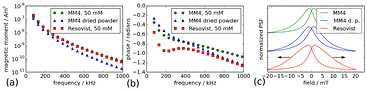
Figure 1. MPS amplitude and phase spectra, and reconstructed point spread functions of MM4, dried MM4 powder, and Resovist. (a) The spectra were generated using an excitation amplitude of 20 mT at a frequency of 25 kHz. (b) Signal phase at odd harmonics. (c) From the amplitude and phase of the spectra, a point spread function (PSF) can be derived. Due to hysteresis effects, the PSFs for the increasing and decreasing fields are not identical. The arrows indicate the direction of field variation for the respective lobe of the PSF.
Download figure:
Standard image High-resolution image2.3. Magnetic particle imaging
2.3.1. MPI measurements.
Imaging was performed using the Philips pre-clinical demonstrator system (Gleich et al 2010). The system has selection field gradients of Gx = Gy = 1.25 T m−1  and Gz = 2.50 T m−1
  . The resulting field free point (FFP) was driven on a 3D Lissajous trajectory with a repetition time of TR = 21.54 ms by applying drive field frequencies of fx = 26.04 kHz, fy = 24.51 kHz, and fz = 25.25 kHz. To reduce the system calibration effort, a quasi-2D volume was covered by applying amplitudes of 16 mT in the x and y direction, but only 1 mT in the z (vertical) direction. Thus, the FFP covered a horizontal 25.6 × 25.6 mm2 plane with a thickness of 0.8 mm. Due to the spatial extent of the PSF, a signal is also generated outside this volume, which is taken into account by using a larger calibration volume as described in the next section. Signals were detected using a dedicated three-axis receiver coil, so that the x, y, and z components of the magnetization were detected simultaneously.
2.3.2. System calibration.
The system functions (SFs) needed for image reconstruction have been determined on a grid of 41 × 41 × 8 voxels of dimensions 1.0 × 1.0 × 1.0 mm3. For each material, an individual SF has been acquired from a small amount of material positioned at the center of the scanner bore, namely 0.8 µl of undiluted Resovist (22 µg(Fe)), 3.1 µl of undiluted MM4 (9 µg(Fe)), and about 0.8 µl of dried MM4 powder (45 µg(Fe)). Focus fields have been used to generate the field offsets corresponding to the desired voxel translations on the imaging grid (Halkola et al 2012). Signals were averaged over 20 Lissajous cycles of duration TR at each position. The calibration procedure yields a SF matrix for each receiver channel, which describes the spectral response (matrix columns) at each spatial position (Rahmer et al 2012). A spectral or frequency component represents a spatial pattern (matrix row) that encodes the respective spatial information. As an example, the real and imaginary parts of a single frequency component (f = 7fx + 2fy ≈ 231.3 kHz) extracted from the x channel SFs have been plotted for the three materials in figure 2.

Figure 2. Gray value plots of the central xy slice of the frequency component corresponding to f = 7fx + 2fy extracted from the x channel system functions (SFs) of Resovist (a, d), MM4 (b, e), and MM4 powder (c, f), respectively. The upper row displays the real part, whereas the lower row displays the imaginary part. Brightness is scaled individually for each material, but the real and imaginary parts have a common scaling. Therefore, one can infer that, for the displayed frequency component of Resovist, the signal in the imaginary part is much higher than in the real part. The relative signal levels in the real and imaginary part are connected to the dynamic magnetization behavior of the respective material.
Download figure:
Standard image High-resolution image2.3.3. Phantom measurements.
A simple phantom has been assembled by combining the three calibration samples in a single plane, as shown in figure 3(a). The materials were filled into cylindrical cavities that were drilled in small plates of plastic with a thickness of 1 mm. The cylinders had a diameter of 1 mm for Resovist and MM4 powder, but a diameter of 2 mm for fluid MM4 to account for the lower concentration. The center-to-center distance of the samples was 10 mm. Figure 3(b) compares the envelopes of the SNR spectra determined from the x channel SFs for the different materials. The SNR measure plotted in the spectrum is the ratio between the overall signal content at a certain frequency component, i.e. the norm over the spatial patterns such as displayed in figure 2, and the noise determined in a background measurement (Rahmer et al 2012). The Resovist sample has about a factor of 2.5 more SNR than the MM4 samples, which both exhibit similar SNR.
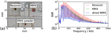
Figure 3. Three-point phantom (a) and envelopes of SNR spectra extracted from the x-channel SFs for the separately measured dots (b). The spatial separation of the dots in the phantom was 10 mm.
Download figure:
Standard image High-resolution imageFor phantom imaging, the MPI sequence described above has been applied without averaging, i.e. the temporal resolution of the scan was TR = 21.54 ms. Four experiments were conducted. In the first, all three materials were measured simultaneously, whereas one material was removed at a time in the following experiments, so that only pairs of materials were scanned simultaneously.
2.3.4. Multi-color reconstruction.
The object measurement yields a signal vector on each channel, so that all three orthogonal field components are considered. These vectors are concatenated to obtain the total signal vector v for one Lissajous cycle TR. The imaging equation determines how a particle concentration vector c is mapped to the signal vector via the system function G:

For reconstruction of the 3D particle concentration in standard MPI, the regularized least-squares problem

has to be solved for the concentration vector c (Knopp et al 2010), where ∥⋅∥ denotes the Euclidean norm. G is the SF matrix that consists of the matrices acquired for the three receiver channels concatenated along the frequency axis. W is a weighting matrix that can be used to select and attach a certain weight to individual frequency components and λ is the regularization factor that is used to adjust the balance between the image resolution and SNR. To minimize noise and to reduce the number of equations, a subset of frequency components is selected for reconstruction by using a threshold on the SNR spectra shown in figure 3(b). Equation (2) is solved using a row-based iterative approach including a non-negativity constraint for the concentration vector (Dax 1993).
If different particle types are measured simultaneously, linearity requires that their signals overlap additively in the signal vector v. For the three different particle types, Resovist, MM4, and dried MM4, with respective system functions GR, GM, and GdM, and concentration vectors cR, cM, and cdM, the imaging equation (1) becomes

This equation shows that the summed signal can be written as a matrix vector product between a matrix of system functions Gc concatenated along the spatial axis and a concentration vector cc consisting of the concatenated individual vectors.
Our approach to separate the different contributions into different images or colors consists of solving the inverse problem for the combined SF Gc and object vector cc. Equation (2) then becomes

or, with explicit notation of the concatenated matrix and vectors:

From the solution vector cc, the 3D particle concentrations for each particle type, i.e. cR, cM, and cdM, can be extracted and can be displayed in separate images or as different colors in a single image.
3. Results
In figure 1(a), Resovist and MM4 display an almost identical signal drop in the MPS spectrum, whereas the signal of MM4 powder drops faster with increasing harmonic number. The frequency dependence of the signal phase shown in figure 1(b) shows more pronounced differences between the materials. Also, the PSF reconstructions in figure 1(c) show clear differences in the hysteresis and shape of the PSF lobes.
The characteristic signal drop observed for the materials in the MPS spectra is also found in the envelope of the SNR spectra shown in figure 3(b). Here, the Resovist signal is higher due to the higher iron concentration in the calibration sample, but the SNR drop is similar for Resovist and MM4, whereas the SNR for MM4 powder drops faster. Despite the high amount of iron, MM4 powder exhibits the lowest performance in both the MPS and MPI measurements, which probably results from particle–particle interactions due to the high iron concentration and from the immobility of the particles in the powder.
Figure 2 displays the spatial signal response patterns of a single frequency component. The patterns of Resovist and MM4 look rather similar in the imaginary part (bottom row) and are almost identical when plotting the magnitude (not shown). However, the real parts differ strongly (top row). For Resovist, the real part exhibits an amplitude almost four times lower than the imaginary part (ratios between the peak-to-peak amplitudes of the imaginary and the real part are 3.8 for Resovist versus 1.2 for MM4 and 1.4 for MM4 powder). Furthermore, the mirror symmetries observed for both MM4 and MM4 powder are broken in the real part pattern of Resovist. One also finds, especially in the data of the imaginary part, that Resovist and MM4 generate rather similar rounded response patterns, while the response of dried MM4 powder exhibits a rectangular spatial structure.
Figure 4 shows the center slice for different reconstructions of a single volume measured from the three-point phantom. First, the data was reconstructed according to (2) using the individual SFs of the three materials (a)–(c). Since in that case, the simultaneously measured signal from three different materials is reconstructed into a single image using only calibration data from one material, not all signals can be assigned correctly and artifacts arise. In this reconstruction, common features shared by all materials are emphasized. Therefore, images (a)–(c) all show three point samples and assign the highest signal to Resovist, which in fact has an amount of iron 2.5 times higher than the fluid MM4 sample and a much better MPI performance than the MM4 powder sample.
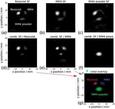
Figure 4. Reconstructed images of the three-point phantom acquired during a single Lissajous sequence. The top row shows reconstruction attempts using the individual SFs for Resovist (a), MM4 (b), and MM4 powder (c), respectively. Since none of the SF matches all the materials, distorted images of all samples are reconstructed. The center row (d)–(f) shows the reconstruction of the three different materials into different images using a combined SF, which assigns most of the signal to the correct sample. Images (a)–(f) are scaled individually to use the full gray scale. (g) shows a color overlay of the three images (d)–(f), where each image is assigned to one color channel.
Download figure:
Standard image High-resolution imageIn the next step, a multi-color reconstruction according to (5) was performed using a combined SF Gc generated by concatenation of the three individual SFs. In that case, an image vector cc results, which is a concatenation of the individual image vectors cR, cM, and cdM, which jointly form the best solution to the inverse problem. The respective images are displayed in figures 4(d)–(f). Although a full separation has obviously not been achieved, this reconstruction clearly assigns more signal to the correct material. A color overlay of the images in (d)–(f) is displayed in (g).
Figure 5 displays color reconstructions of measurements, where only two different materials were measured simultaneously. Consequently, only the two respective SFs were combined in (5). The overlay images (a)–(c) assign different colors to the images reconstructed for each material. From the intensity profiles through the objects (d)–(f), one finds that separation works very well between fluid MM4 and MM4 powder as well as between Resovist and MM4 powder. Separation between Resovist and fluid MM4 is not as good, but good enough for visual discrimination in the image (b).
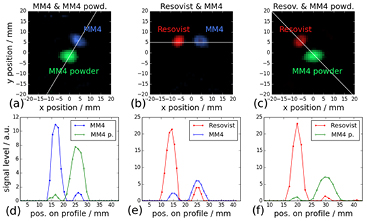
Figure 5. Color MPI reconstruction of measurements of only two materials (a)–(c) and a signal intensity profile through the respective two point sample position (d)–(f). The position of the profile is indicated by the thin white lines in (a)–(c).
Download figure:
Standard image High-resolution imageAs a measure of the quality of separation, one can determine the ratio between the peak height at the correct versus the wrong signal position along the profile. In (d), the ratio is 9.3 for MM4 and 8.5 for MM4 powder. In (e), the ratios are 5.4 and 2.7 for Resovist and MM4, respectively. In (f), one finds 16.1 and 6.2 for Resovist and MM4 powder, respectively.
4. Discussion
The similarity in the MPS amplitude spectrum between Resovist and MM4 (see figure 1(a)) could be explained by a similar distribution of particle sizes resulting from the synthesis method, which for both materials is precipitation from aqueous solution in the presence of carboxy-dextran or dextran. If particle discrimination is based on differences in the colinear and transverse PSFs which depend on particle diameter, a similar size distribution would mean that the two materials should be very hard to separate at all. Only dried MM4 powder shows a markedly different behavior in the amplitude of higher harmonics. When comparing the phase of the harmonics (see figure 1(b)), one finds differences between all three materials. In the frequency range up to 400 kHz, the phase of the Resovist harmonics clearly differs from that of the MM4 materials. Consequently, differences between Resovist and the MM4 materials are also found in the 1D PSFs (see figure 1(c)), whose reconstruction includes amplitude and phase information. These hysteresis-related phase effects may facilitate the separation of the signals generated by the two types of material.
In the spatial patterns of the SF frequency components (see figure 2), the difference in real part amplitude and symmetry between Resovist and the MM4 materials should be linked directly to the different hystereses and shapes observed in the PSFs. The time domain representation of the SF is closely related to a series of instantaneous PSFs for each time sample acquired during an FFP trajectory cycle. Therefore, differences in the instantaneous PSFs lead to differences in the complex spectral representation of the SF shown in figure 2. Due to the curved path of the applied Lissajous trajectory, the instantaneous PSFs represent mixtures between the colinear and transverse PSFs (see appendix
Regarding the shape of the SF patterns displayed in figure 2, the rectangular patterns found for dried MM4 powder are more similar to the results obtained from simulations based on the Langevin magnetization curve for isotropic particles and approximations of the patterns using tensor products of Chebyshev functions (Rahmer et al 2012). Since Brownian rotation is suppressed in dried material, it follows that the rounded patterns for Resovist and MM4 are probably related to particle reorientation.
The multi-color reconstruction of the three-point phantom shows that a reasonably good discrimination between the samples can be achieved in the MPI measurement, see figures 4(d)–(f). The image of MM4 powder only shows a signal from the sample containing MM4 powder, i.e. the signal from fluid samples is correctly assigned to the other images. Obviously, the differences between fluid and solid materials are large enough to enable this separation. This may be linked to the differences in spatial patterns that solid MM4 powder exhibits in comparison with the fluid materials in the SFs as shown in figure 2. On the other hand, some of the signal of MM4 powder is showing up in both the Resovist and the fluid MM4 image, so separation is not fully symmetric. At this point, more experimental work with different particle types and also simulations are necessary to reach an understanding of the effect. This is, however, beyond the scope of this initial experimental work. The signal separation between Resovist and fluid MM4 is not as good, especially when looking at the MM4 image (cf. figure 4(e)). This is in line with results from the MPS and SF evaluation, which show that Resovist and MM4 behave very similar, except for differences in phase behavior. To optimize the separability of fluid materials, future investigations should try to identify particle types with strongly differing signal responses, e.g. due to differing particle size and anisotropy distributions or due to different coatings (Khandhar et al 2013, Starmans et al 2013).
In a typical imaging scenario, one would probably want to discriminate only two signal origins, e.g. a catheter versus blood or bound versus freely floating particles. This situation has been mimicked by imaging only two materials at the same time as shown in figure 5. In that case, the assignment of signals to the correct material is significantly better than for the combination of three materials. While the separation between MM4 powder and the fluid materials is very good (ratios between peaks of correct and wrong assignment are above 8.5), separation between Resovist and MM4 is not as good (ratio is only 2.7 for MM4), again owing to the similarity of the materials.
In the multi-color images, one can observe that the image of the point sample of the dried MM4 powder has a larger diameter than the other samples, although its true diameter is the same as for the Resovist sample. This may be attributed to the lower resolution achievable with solid MM4 powder, which is a consequence of the faster drop in the amplitude of higher harmonics observed for this material in the MPS spectrum (cf. figure 1(a)) and the SNR spectrum (cf. figure 3(b)). As higher harmonics represent finer spatial detail, a reduction in their SNR directly translates to lower resolution.
The initial results presented in this work indicate that the separation of at least two particle types measured simultaneously is feasible with currently available particles. Thereby, no modification of the system hardware or measurement sequence is required. In particular, the high temporal resolution of the MPI measurement is not affected. The additional effort required for multi-color MPI is limited to the acquisition of SFs for each material and larger matrices to be handled in reconstruction. However, many questions remain to be addressed regarding the quality and reliability of signal separation.
For instance, the relative importance of the potential mechanisms for particle discrimination has to be determined. Differences in size distribution as well as differences in the hystereses of the magnetization curves and their effects on the relevance of Brownian versus Néel relaxation have to be considered. As discussed in appendix
A further point to investigate is the separation of signals from particles residing in the same voxel. This would be important for the discrimination between targeted particles attached to a lesion and free particles passing nearby in the blood stream. Also, a potential dependence of the quality of separation on the spatial position within the field of view, resulting from a non-homogeneous FFP trajectory such as the Lissajous trajectory, should be investigated.
An important point to consider is quantitativeness. While MPI reconstruction for a single particle type is quantitative (Weizenecker et al 2007, Lu et al 2013), it has to be shown whether this holds for multi-color MPI as well. Clearly, a signal assigned to the wrong material destroys quantitativeness. However, if a very good separation between the signals is achieved, one should assume that the individual images are quantitative. For instance, the results presented for two-color MPI in figures 5(b) and (e) correctly reproduce the higher amount of iron in the Resovist sample, however, more evidence has to be gathered on the reliability of the approach with respect to quantitation.
There are many applications that could benefit from multi-color MPI. With regard to the application of MPI in cardiac interventions (Haegele et al 2012), it could be used to differentiate between a catheter (impregnated with immobilized particles (Rahmer et al 2013b)) and blood (free flowing particles or particles encapsulated in red blood cells (Antonelli et al 2011, Rahmer et al 2013a)). In that context, it could have a further use in labelling stents with a third type of particle. For gastro-intestinal applications, magnetic devices have been suggested that can be steered using the magnetic fields of an MPI system (Carpi et al 2011, Nothnagel et al 2013). Here, multi-color MPI could visualize the device's position and the gastro-intestinal tract at the same time, if its lumen has been labeled beforehand using a diet containing iron-oxide particles. More generally, it may be of interest to simultaneously visualize and discriminate different compartments of the body, such as the blood system, the lymphatic system, the gastrointestinal tract, or a specific organ, by loading them with different particle types.
Among the applications that do not probe different particle types, but different particle environments, an obvious example would be the discrimination between free flowing and targeted particles attaching to some lesion of interest (Rauwerdink and Weaver 2010a). Moreover, the detection of blood coagulation could be of interest (Murase et al 2014), for instance in the case of a hemorrhagic stroke. More generally, any relevant change in the particle spectrum can potentially form the basis for particle discrimination, so that changes in viscosity, pH value, or temperature may be accessible. Signal separation based on many of these effects has already been shown spectroscopically (Weaver et al 2009, Rauwerdink and Weaver 2010b). The approach presented in the current work would allow for combining them with imaging. A potential application that could arise from this combination is the simultaneous visualization and temperature measurement based on the signal generated from particles used in magnetic hyperthermia applications (Thiesen and Jordan 2008).
5. Conclusion
Initial experimental results on the separability of signals measured simultaneously from different particle types have been presented. A system-function-based reconstruction approach reconstructs separate images for different particles, which can then be combined into a single color-coded image. In view of the rather high similarity of the materials under investigation, a promising separation has been achieved based on data acquired in only a small fraction of a second. Many aspects regarding the understanding and optimization of the effects that enable particle separation require further investigation, but it is obvious that multi-color MPI can be useful for many applications in the fields of medical imaging, intervention, and therapy.
Acknowledgments
The authors acknowledge funding by the German Federal Ministry of Education and Research (BMBF) under the grant numbers 13N9079 and 13N11086.
Appendix A: Background on particle discrimination
The characteristics of the particles enter the detected MPI signal via a 3D kernel that is convolved with the spatial information. This kernel is related to the magnetization curve and its derivative; its width depends on the steepness of the magnetization curve and limits the achievable spatial resolution. Its 3D shape has been determined for the cases of ideal particles having a step-like magnetization curve (Rahmer et al 2009) and for particles with a Langevin magnetization curve (Goodwill and Conolly 2011). For different particle types to be discerned, their respective MPI signal must differ. To find the requirements for signal differences, the time domain signal equation is investigated in the following.
A.1. MPI signal equation for multiple particle types
The signal s(t) detected by a coil with sensitivity b(r) from a concentration distribution ρ(r) of particles with individual magnetization m is given by Goodwill and Conolly (2011):

Thereby, h(r) is a matrix representing the shape of the 3D kernel or the point spread function (PSF) which is convolved in 3D with the particle distribution. The spatial position r and velocity  are probed at the position rs(t) of the field free point (FFP).
When two different particle types are probed, the superposition of their signals is detected:

If one PSF can be generated from the other PSF by convolution with a fictitious distribution function ρf(r),

one could assign all signals to one particle type without any effect on the generated signal
Specifically, particle distributions ρ1(r) and ρ2(r) with two different particle types would generate the same signal as ρ1(r)***ρf(r) + ρ2(r) of only the second particle type, so that it would be impossible to discern the two particle types.
Analytically, it is known that Gaussian curves are convolution invariant, so that if the PSFs in (A.3) were Gaussians of different widths, convolution with a Gaussian distribution ρf(r) would translate the narrower curve into the broader one. As the PSF is related to the derivative of the magnetization curve, it has a bell-shape which is quite similar to a Gaussian. Therefore, it may be the case that particles cannot be discerned at all.
To really test whether PSFs satisfy (A.3), a Langevin magnetization curve is assumed and different scenarios are calculated numerically. The Langevin curve applies to simple spherical particles (Bean and Livingston 1959), which can only differ in diameter or saturation magnetization, both of which affect the width of the resulting PSF. For particles of the same material and saturation magnetization, it is tested whether one can separate the signal of particles with different core diameters. For simplicity, linear FFP trajectories are used, so that the FFP velocity  is always aligned along one direction. Together with the sensitive direction of the detecting coil, b(r), the velocity vector determines which component is selected from the PSF matrix in (A.1).
A.2. 1D MPI with colinear detection
In the first step, a colinear arrangement of detection coil sensitivity and drive field trajectory line along x is assumed. Then, the colinear PSF component h∥(r) has to be considered, which is given by Goodwill and Conolly (2011):

The PSF is the sum of a term containing the derivative of the Langevin magnetization curve,  , and a term containing the magnetization curve
  itself. A three-dimensional spatial dependence enters the colinear PSF via the field magnitude H (r). κ is a particle dependent factor that contains the vacuum permeability μ0, the single particle magnetic moment m, and the product between the Boltzmann constant kB and the temperature T. For spherical particles with magnetic core diameter d and volume V, the magnetic moment is given by m = VMS = (π d3/6) MS, where MS is the saturation magnetization of the material given in T/μ0. Thus, κ is proportional to the 3rd power of the particle diameter d. Since κ only appears in products with selection field gradient components Gi, the effect of different particle diameters is similar to scaling the gradients and thus scaling the spatial extent of the PSF in all three dimensions.
For 1D line imaging on the trajectory line, i.e. y = z = 0, the second term vanishes and one arrives at a simplified equation:

Figure A1(a) displays the PSFs for particle diameters 22 and 30 nm, respectively. However, as figure A1(b) shows, a broad PSF, which would be the 1D image of a point-like sample of 22 nm particles, can always be modeled by a linear superposition of narrow PSFs resulting from a spatial distribution ρf(r) of 30 nm particles along the FFP trajectory line. The distribution function has been calculated numerically by Wiener deconvolution of the narrow from the broad PSF. It follows that (A.4) holds true and the signal response in both cases is identical, so that the two particle types cannot be discerned in this 1D experiment.
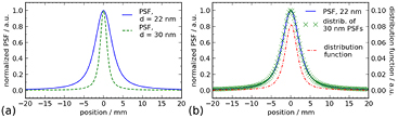
Figure A1. 1D point spread functions (PSFs) for Langevin particles calculated as the derivative of the magnetization curve. (a) PSFs for two different particle core diameters (other parameters used for the calculation: T = 300 K, Gx = 1.25 T m−1, and MS = 0.6 T). (b) The broad PSF (solid line) can be matched by a linear superposition of narrow PSFs (crosses) using a smooth spatial distribution function of 30 nm particles (the dash–dotted line). Therefore, these two situations cannot be discerned in 1D MPI with colinear detection.
Download figure:
Standard image High-resolution imageIf the FFP motion is not limited to a single line, but extended to a 2D or 3D set of parallel lines, a 2D or 3D PSF according to (A.5) arises.
For ease of presentation, a 2D imaging scenario of a planar object is considered in the following, but the investigation could be done analogously in 3D.
In figures A2(a) and (b), the 2D PSF in the xz plane calculated according to (A.5) is shown for particle diameters 22 and 30 nm, respectively. The PSF is positive-valued and the broad PSF (a) is a scaled version of the narrow PSF (b). If it were possible to mimic the broad PSF by a spatial distribution of narrow-PSF particles, similar to the 1D situation shown in figure A1(b), particles with different diameters could not be discerned. A 2D Wiener deconvolution has been performed to arrive at such a distribution function (c). From a difference plot (e), one finds that the resulting distribution of narrow PSFs (d) matches the original PSF extremely well. This would mean that even when considering the 2D PSF, particles cannot be discerned. However, the resulting distribution also relies on negative values, which would require non-physical negative particle concentrations. Consequently, if a 2D (or 3D) image of particles with different core diameters is acquired using the linear trajectory, it should be possible to at least partially discern particles when using a non-negativity criterion in the reconstruction algorithm. The quality of the separation will thereby depend on the difference in the core diameters and the available SNR.

Figure A2. 2D PSF investigation. PSFs in the xz plane with excitation in x direction and distribution functions are displayed. Parameters used for the calculation: T = 300 K, Gx = 1.25 T m−1  , Gz = 2 Gx, and MS = 0.6 T
  . (a, b) Colinear PSFs according to (A.5) for particle core diameters 22 and 30 nm, respectively. Different diameters lead to a spatial scaling of the PSFs. (c) Distribution function obtained by Wiener deconvolution of narrow PSF (b) from broad PSF (a). (d) Broad PSF calculated by convolution of narrow PSF (b) with distribution function (d). (e) The difference between original (a) and reconstructed (d) broad PSF. (f) Broad PSF calculated by convolution of narrow PSF (b) with distribution function (j) obtained from transverse PSF. (g) The difference between original (a) and reconstructed (f) broad colinear PSF. (h, i) Transverse PSFs according to (A.7) for diameters 22 and 30 nm, respectively. (j) Distribution function obtained by Wiener deconvolution of narrow PSF (i) from broad PSF (h). (k) Broad PSF calculated by convolution of narrow PSF (i) with distribution function (j). (l) The difference between original (h) and reconstructed (k) broad PSF. (m) Broad PSF calculated by convolution of narrow PSF (i) with distribution function (c) obtained from the colinear PSF. (n) The difference between original (h) and reconstructed (m) broad transverse PSF. Note: the value range of all images is symmetric between positive and negative values, so that zero is at the center of the color spectrum. Distribution functions have been scaled individually and then multiplied by a factor to visualize values close to zero. The difference images take their scaling from the respective PSFs, but have also been multiplied by a factor.
Download figure:
Standard image High-resolution image
A.3. 1D MPI with transverse detection
If the detection coil is mounted to pick up the field component transverse to the trajectory line, the spatial pattern of the signal response changes. Assuming detection of the z component of the magnetic field while applying a drive field in x direction, the transverse component of the PSF h⊥(r) is given by Goodwill and Conolly (2011):

Figures A2(h) and (i) shows the xz plane of transverse PSFs for particle diameters 22 and 30 nm, respectively. For the transverse PSFs, the signal response is zero along the symmetry lines and changes sign between the quadrants. In figures A2(h)–(l), the above evaluation is repeated for the transverse PSF. The distribution function (j) obtained by Wiener deconvolution relies heavily on negative values, so that again, a non-negativity constraint would enable particle discrimination.
The MPI scanner used in this work is capable of detecting all three orthogonal field components simultaneously. Therefore, a fictitious distribution function ρf(r) that would make particles indiscernible would have to be the same for all detection directions. Figure A2 displays reconstructed PSFs (f, m), which result from the convolution of the colinear PSF (b) with the distribution obtained from the transverse PSFs (j), and from the inverse case involving (i) and (c), respectively. The difference images (g, n) show that these PSFs differ strongly from the original ones. Therefore, as colinear and transverse detection require different fictitious distribution functions, one can expect that the simultaneous reconstruction of a signal from orthogonal receiver channels improves the separability of particles with different diameters.
Regarding the influence of the trajectory type, one can speculate that curved trajectories may further improve the separability of particles, however, an investigation of the influence of the trajectory is beyond the scope of this work.
A.4. Hysteresis effects
So far, only isotropic particles have been discussed, but particle cores vary in shape and composition. In a simplified picture, this can be taken into account by introducing anisotropy by allowing the core to have the shape of a prolate spheroid, i.e. an ellipsoid of revolution (Weizenecker et al 2012). The resultant effect is that for the Néel part of the magnetization, the applied field must counteract the anisotropy field to be able to reorient the particle magnetization. This leads to a hysteresis in the magnetization curve which splits the PSFs into two lobes, one for the magnetization flipping forward with increasing field and one for the magnetization flipping backwards with decreasing field. Different materials have different anisotropy distributions, and therefore, differ in the shift and shape of the PSF lobes (see figure 1(c)). In the frequency domain, hysteresis affects the phase of the detected signal. Simulations show that in a simple 1D experiment, hysteresis-related phase differences alone already enable partial signal separation (Schmale et al 2010). Therefore, one can expect that the hysteresis effects deliver additional information that further supports the separation of signals from different particle types.