
Abstract
Accurate and efficient scatter correction is essential for acquisition of high-quality x-ray cone-beam CT (CBCT) images for various applications. This study was conducted to demonstrate the feasibility of using the data consistency condition (DCC) as a criterion for scatter kernel optimization in scatter deconvolution methods in CBCT. As in CBCT, data consistency in the mid-plane is primarily challenged by scatter, we utilized data consistency to confirm the degree of scatter correction and to steer the update in iterative kernel optimization. By means of the parallel-beam DCC via fan-parallel rebinning, we iteratively optimized the scatter kernel parameters, using a particle swarm optimization algorithm for its computational efficiency and excellent convergence. The proposed method was validated by a simulation study using the XCAT numerical phantom and also by experimental studies using the ACS head phantom and the pelvic part of the Rando phantom. The results showed that the proposed method can effectively improve the accuracy of deconvolution-based scatter correction. Quantitative assessments of image quality parameters such as contrast and structure similarity (SSIM) revealed that the optimally selected scatter kernel improves the contrast of scatter-free images by up to 99.5%, 94.4%, and 84.4%, and of the SSIM in an XCAT study, an ACS head phantom study, and a pelvis phantom study by up to 96.7%, 90.5%, and 87.8%, respectively. The proposed method can achieve accurate and efficient scatter correction from a single cone-beam scan without need of any auxiliary hardware or additional experimentation.
Export citation and abstract BibTeX RIS

Content from this work may be used under the terms of the Creative Commons Attribution 3.0 licence. Any further distribution of this work must maintain attribution to the author(s) and the title of the work, journal citation and DOI.
1. Introduction
With the commercialization of large-area flat-panel imagers, CBCT imaging has been increasingly and widely employed in various applications including image-guided surgery and radiotherapy (Ning et al 2000, Jaffray et al 2002, Oldham et al 2005, Daly et al 2006, Dawson and Jaffray 2007). However, CBCT images suffer from scatter due to the wide cone angles. Scatter, one of the dominant sources of image artifacts in CBCT, leads to degradation of image quality relative to that of fan-beam CT images. Therefore, numerous scatter correction methods have been developed (Ning et al 2004, Zhu et al 2005, Siewerdsen et al 2006, Zbijewski and Beekman 2006, Zhu et al 2006, Chen et al 2009, Poludniowski et al 2009, Jin et al 2010, Niu and Zhu 2011, Ruhrnschopf and Klingenbeck 2011a, 2011b, Lee et al 2012). The deconvolution method is one of those scatter correction methods that estimates the scatter component by convolving projection data with a spatially invariant scatter kernel model. This method has several advantages, among which are dispensability of additional scanning efforts or additional hardware, and computational efficiency. Monte Carlo methods by contrast, though usually providing accurate scatter estimation in CBCT, trade off accuracy and computational cost (Zbijewski and Beekman 2006, Chen et al 2009, Poludniowski et al 2009, Ruhrnschopf and Klingenbeck 2011a). Accordingly, in practical CBCT applications, deconvolution-based scatter correction methods, where the accuracy of the scatter correction in a given imaging task is acceptable, have been widely utilized.
The accuracy of the deconvolution method largely is a function of the scatter kernel and its parameters. A scatter kernel model usually requires adjustment of many parameters, the empirical determination of which can be challenging, particularly considering diverse clinical situations. A precise and convenient optimization process for determination of parameters, therefore, is highly desirable. In this work, we made use of the data consistency to determine such parameters effectively. The data consistency condition (DCC), which is the zeroth-order form of the Helgason–Ludwig (HL) condition (Helgason 1980, Natterer 2001), indicates that the total sum of the projection data in parallel-beam geometry is a constant that is independent of the view-angle. Data consistency, however, is problematic, due to physical CBCT factors such as scatter, beam-hardening, and suboptimal calibration. Under the condition that other factors are either managed within a tolerable level or can be neglected, the DCC will depend largely on the scatter component. As will be shown in the Results and Discussion sections below, beam-hardening in CBCT, compared with scatter, is relatively minor in its effect on data consistency. Therefore, data consistency can be used to determine the degree of scatter correction and to steer the update in iterative kernel optimization.
In order to apply the zeroth-order form of the HL condition in CBCT, one has to look into the sum of the line integrals in the mid-plane of cone-beam data after fan-parallel rebinning (Kak et al 1988). Mid-plane cone-beam data basically is fan-beam data, and a rebinning process that converts the fan-beam to parallel-beam renders the data to meet the DCC. The DCC can then be used in each iterative step of scatter kernel modification to secure that the optimal scatter kernel can be reached. For iterative optimization of scatter kernel parameters, we employed the so-called particle swarm optimization (PSO) algorithm (Kennedy and Eberhart 1995, Yuhui and Eberhart 1998, Parsopoulos and Vrahatis 2002, Trelea 2003). The PSO algorithm, one of the meta-heuristic optimization algorithms that imitates the foraging process of animals, has advantages such as including fast convergence and simplicity of implementation. We demonstrated, by means of a simulation study using the thoracic part of the XCAT phantom (Segars et al 2010) as well as experimental studies using the ACS head phantom and the pelvic part of the Rando phantom, that data consistency can be a useful scatter kernel optimization criterion that can help, subsequently, to improve scatter correction.
2. Methods
2.1. Deconvolution method
The deconvolution method assumes that the scatter component can be estimated by a spatially invariant convolution of the primary signal with a scatter kernel (Love and Kruger 1987, Seibert and Boone 1988, Ohnesorge et al 1999, Li et al 2008, Ducote and Molloi 2010, Sun and Star-Lack 2010). The scatter kernel, which is based on the physical model, determines the magnitude and distribution of the scatter component in the projection data. The accuracy of the deconvolution method is largely a function of the shape of the scatter kernel. Various scatter kernel models have been proposed for estimating scatter components and for improving the accuracy of deconvolution method. In the present work, we used a symmetric scatter kernel proposed by Ohnesorge (Ohnesorge et al 1999) and modified by Sun (Sun and Star-Lack 2010), for convenience of implementation in the PSO framework. The symmetric scatter kernel or point spread function  follows the model consisting of an amplitude factor
  and a form function
  as shown below:


The spatial position r = xi + yj is defined on the detector,  is the unattenuated intensity signal, and
  is the attenuated primary signal. The parameters
  and
and  are the fitting parameters that determine the scatter kernel shape. These parameters can be fit empirically from measurements or simulations of pencil beams directed through the water-equivalent phantoms, which can be cumbersome and suboptimal in various scanning tasks.
The scatter estimate at position  can be acquired via the 2D convolution operation:

where  is the primary estimate,
  is the amplitude factor defined in equation (1), and
  is the form factor defined in equation (2).
From equation (4), one can estimate the scatter component of the projection data and can obtain scatter-corrected data by subtracting the estimated scatter from the measured data. In the present work, we used the measured intensity signal I as the initial primary estimate, after which we iteratively estimated the primary intensity. Typically, three iterations are known to be sufficient for the primary intensity recovery (Sun and Star-Lack 2010).
The key purpose of our work was to determine the fitting parameters of the symmetric scatter kernel using the DCC without any further empirical processes or hardware implementation. As the accuracy of scatter deconvolution is affected by the scatter kernel parameters, we optimized them iteratively using the DCC as the criterion.
2.2. Data consistency condition (DCC)
Various versions of the DCC have been derived and utilized for diverse purposes (Patch 2002, Chen and Leng 2005, Yu et al 2006, Xu et al 2010, Tang et al 2011). The most well-known DCC are the Helgason–Ludwig (HL) conditions, which apply to the Radon transform in parallel projection geometry. The zeroth-order HL condition specifies that the total attenuation in a parallel-beam geometry such as that shown in figure 1 should remain constant from view to view. In other words, if we sum up the measured parallel projection data for each view, the sum should be a constant that is independent of the view-angle.

Figure 1. Rotated coordinate system in parallel-beam geometry.
Download figure:
Standard image High-resolution imageIn order to apply this condition to scatter kernel optimization, we used the mid-plane of cone-beam projection data after each deconvolution. We converted the fan-beam projection data to parallel-beam data by use of fan-parallel rebinning (Kak et al 1988), because the zeroth-order HL condition is valid only in parallel-beam geometry.
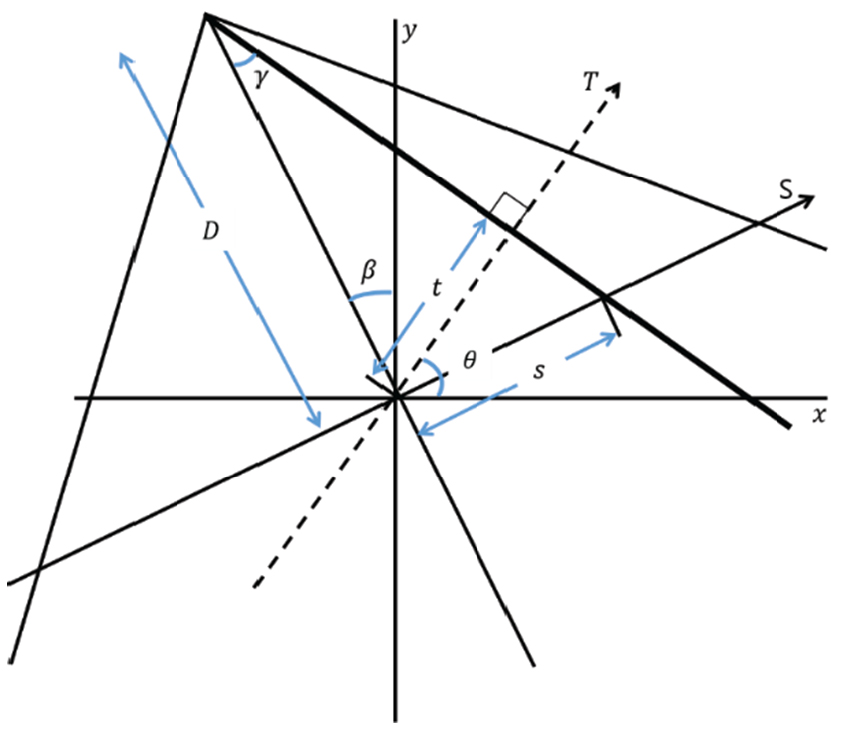
2.3. Fan-parallel rebinning
Both fan- and parallel-beam geometries are shown in figure 2. β represents the fan-beam source angle,  represents the fan-angle,
  represents the corresponding parallel-beam angle, and
  represents the radial parallel coordinate.
  represents the virtual fan-beam detector coordinate and
  is the distance of the source point from the origin.

Figure 2. Geometries of fan- and parallel-beam for rebinning.
Download figure:
Standard image High-resolution imageThe relationship between ( ) and (
 ) is given by equations (5) and (6), below.


2.4. PSO algorithm
The key step in this work is to find, using the DCC as the criterion, the optimum scatter kernel parameters. While the parameters values are iteratively changed, the optimum that best satisfies the DCC is sought. However, this strategy can be challenging with respect to its computational burden if all of the possible parameter values in a certain range need to be checked in a combinatorial fashion.
For efficient implementation of the optimization process, we incorporated the PSO algorithm (Kennedy and Eberhart 1995, Yuhui and Eberhart 1998, Parsopoulos and Vrahatis 2002, Trelea 2003). The PSO algorithm is an optimization algorithm that finds the best element from sets of available alternatives. PSO simulates the foraging process of certain animals; it is a meta-heuristic, in that it makes few assumptions for problem optimization and can search large spaces of candidate solutions. The PSO algorithm, in comparison with other algorithms, offers the advantages of simplicity in implementation and relatively fast convergence.
In PSO, an individual solution is expressed as a 'particle', and a solution group is expressed as a 'swarm'. There are two conditions that need to be met in the PSO algorithm. Particles, which stand for individuals in a swarm, should share information with each other during iterations. Also, they should move based on that shared information. When better positions of agents are found, the movement of the swarm will be updated and guided accordingly. This process is repeated until a satisfactory solution is reached within a reasonable number of iterations. In our study, we had six parameters in the scatter kernel; therefore, we set the number of swarms as 6, and for each swarm we set the number of particles as 20. A schematic illustration of a particle and a swarm is provided in figure 3, and the movement of a particle in an update step is indicated in figure 4.

Figure 3. Particles and swarm in the PSO algorithm.
Download figure:
Standard image High-resolution image
Figure 4. Position and velocity update  of
of  particle in swarm.
Download figure:
Standard image High-resolution imageIn figure 3,  represents the index of a parameter, and
  represents the index of a single candidate of a parameter. Each particle or candidate of a parameter has an initial position vector and velocity vector. The position vector
  represents the value of a parameter, and the velocity vector
  depicts the increment of the parameter value. The superscript 'now' and 'next' represent the generations of the iteration. Each particle is evaluated by the cost function, which is the satisfaction level of data consistency as will be explained in the following section. The movements of particles are determined by equations (7) and (8).


where  represents the position vector that has the best value of the
  particle, and
  represents the position vector that has the best value in the swarm.
  represents the random number uniformly distributed in the range [0, 1].
  is a parameter called the inertia weight parameter, which is employed to accommodate the impact of the previous velocity on the current one. We initialized
  by 1 and decreased it toward 0 as the number of iterations increased. The inertia weight is known to help global searching in the early iterations as well as fine searching in the last search toward the global optimum.
  and
and  are positive constants that are used to limit the velocity vectors; in this study, we set both
  and
and  to 0.5, which was the suggested value (Parsopoulos and Vrahatis 2002). As meta-heuristic algorithms, including the PSO algorithm, do not guarantee the global optimum in general, we incorporated the inertia weight and the positive constants in the algorithm implementation in this work to gear toward the global optimum. With these enforcing schemes, the PSO is known to have a better chance of finding the global optimum within a reasonable number of iterations, as discussed in Parsopoulos and Vrahatis (2002). In this way, it is likely that the global optimum can be reached empirically for the six parameters of the scatter kernel. We randomized the position and velocity vectors in the initialization step within a reasonable range, referencing Sun's work (Sun and Star-Lack 2010) to guide the ranges of the positions and velocities.
2.5. Workflow
A conceptual workflow of the proposed scatter kernel optimization method is summarized in figure 5.

Figure 5. Pipeline of proposed scatter kernel optimization method.
Download figure:
Standard image High-resolution image2.6. Experimental conditions
To validate the proposed method, we performed both simulation and experimental studies. In the simulation study, the thoracic part of the XCAT numerical phantom (Segars et al 2010) was used. We acquired scatter-free projection data for 360 views, and added scatter noise by convolving the scatter-free data with a specific scatter kernel. For the scatter calculation, a spatially variant kernel that considers the object thickness was employed, referencing Sun (Sun and Star-Lack 2010) again to determine the parameters of multiple thickness groups. Although scatter kernel information is thus available, for the purposes of scatter correction, we assumed it to be unknown. The recovery of the scatter kernel parameters in the simulation study appeared to be very useful for at-a-glance assessment of optimization algorithm performance. However, since the scatter kernel model used for correction in this work is composed of a multiplicative part to and a convolving part with the primary signals, one-shot deconvolution in the Fourier domain would not work in this approach; instead an iterative deconvolution, as described above, is usually used. Since the iterative deconvolution method applies consecutive convolution and subtraction to the measured data, which contains both primary and scatter signals, the convolution kernel is likely to be different from the kernel that was used for scatter generation in the simulation study. It is particularly so because the kernel used in the scatter generation process employs a thickness-dependent model, whereas the kernel used in the deconvolution process assumes a spatially invariant model in this work. The x-ray tube voltage in the simulation study was set to 140 kVp. A system geometry for the simulation study is indicated in table 1.
Table 1. System geometry for simulation study.
| Parameter | Value |
|---|---|
| Source-to-isocenter distance | 530 mm |
| Source-to-detector distance | 1000 mm |
| Detector matrix size | 1024 × 1024 |
| Detector pixel size | 0.75 mm |
In the experimental studies, we used a bench-top CBCT system, the scanning parameters of which are summarized in table 2. The system consists of an x-ray tube (NDI-451, Varian Co., Salt Lake City, Utah, USA) and a flat panel detector (1642AP, Perkin Elmer, Santa Clara, California, USA). An aluminum wedge filter was used in order to make a uniform beam quality. Neither a bowtie nor an anti-scatter grid was employed in the experiments. A PH-3 angiographic CT head phantom ACS (Kyoto Kagaku Co., Ltd, Kyoto, Japan) and the pelvic part of the RT-humanoid phantom (the Rando phantom, Humanoid Systems, Carson, California, USA) were utilized in the experiments. Using these phantoms, we acquired not only cone-beam projection data but also fan-beam data by collimating the x-ray beam to secure, by inherent scatter suppression, almost scatter-free reference data. The x-ray tube voltage was 140 kVp and the number of projection views was 360, as in the simulation study.
Table 2. System geometry for experimental studies.
| Parameter | Value | |
|---|---|---|
| ACS head | The pelvic part of the Rando | |
| Source-to-isocenter distance | 1700 mm | 1900 mm |
| Source-to-detector distance | 2250 mm | |
| Detector matrix size | 1024 × 1024 | |
| Detector pixel size | 0.4 mm | |
3. Results
3.1. Simulation study
In the scatter-free projection data, the DCC was well satisfied as shown in figure 6(a), though there was a slight variation, possibly due to the beam-hardening and the partial volume effects. Contrastingly, in the scatter-contaminated case, there was a large variation in the sum of line integrals from view to view, and in fact, lowered values can be seen in figure 6(b). This variation and reduction in the sum of line integrals was due mostly to the added scatter. Figure 6(c) plots the sum of line integrals of the scatter-corrected data by use of the proposed method; as is apparent, the DCC was fairly well recovered. As a quantitative metric that can be used for a cost function, we introduced the inconsistency level defined in equation (9). The inconsistency level represents the percentage of standard deviation with respect to the average. A low inconsistency level implies that the DCC is highly satisfied.


Figure 6. Plots of sum of line integrals of (a) scatter-free projection data, (b) scatter-contaminated projection data, and (c) scatter-corrected projection data as function of view number.
Download figure:
Standard image High-resolution imageTable 3 shows the inconsistency levels for the respective cases. The difference in the inconsistency level of the scatter-contaminated data with respect to the scatter-free data was calculated as  , and similarly, the corresponding value of the scatter-corrected data was
  . Table 4 shows the selected parameters of the scatter kernel for the optimum DCC condition in the simulation study.
Table 3. Inconsistency level of each case in XCAT simulation study.
| (a) Scatter-free | (b) Scatter-contaminated | (c) Scatter-corrected | |
|---|---|---|---|
| Inconsistency level (%) | 0.529 | 2.781 | 0.637 |
Table 4. Optimally selected parameters of scatter kernel in simulation study.
 |
 |
 |
 |
 |
 |
|---|---|---|---|---|---|
 |
 |
 |
 |
 |
 |
Figure 7 shows the converging behavior of the inconsistency level as the number of iterations increases by use of the PSO algorithm. We used  for
for  to demonstrate the converging nature, but a higher value can be used in practical applications so as to stop at earlier iterations.

Figure 7. Plot of inconsistency level with respect to iteration number in simulation study.
Download figure:
Standard image High-resolution imageThe reconstructed images on the mid-plane and off-mid-plane from the scatter-free, scatter-contaminated, and scatter-corrected projection data and their line profiles along the solid lines are shown in figures 8 and 9, respectively. Both on the mid-plane and off-mid-plane, image artifacts caused by the scatter component are clearly seen in figure 8(b) and in the dotted line profile in figure 9; such artifacts were substantially mitigated by use of the proposed method.

Figure 8. Reconstructed images of (a) scatter-free, (b) scatter-contaminated, and (c) scatter-corrected projection data of XCAT phantom. The display window is [0.013  , 0.03
  ]. Upper row: reconstructed images of mid-plane at
  cm; bottom row: reconstructed images of off-mid-plane at
  cm.
cm.
Download figure:
Standard image High-resolution image
Figure 9. Line profiles of reconstructed images on mid-plane (a) and off-mid-plane (b) from scatter-free, scatter-contaminated, and scatter-corrected data.
Download figure:
Standard image High-resolution imageFor a quantitative assessment of image quality, we used structure similarity (SSIM), which is a metric that evaluates the similarity between two images. For comparison of the scatter effects between cases, contrast also was calculated. Region of interests (ROIs) that we used for the assessments are indicated in figure 8. The results of the quantitative assessment of each case are summarized in tables 5 and 6. On the mid-plane images, the optimally selected scatter kernel improved the contrast up to 99.4% and the SSIM up to 99.8% from 75.1% and 70.4% in the scatter-contaminated images, respectively. Similarly on the off-mid-plane images, the scatter correction improved the contrast up to 99.5% and the SSIM up to 99.8% from 82.3% and 66.0% in the scatter-contaminated images.
Table 5. SSIM of reconstructed images of XCAT phantom.
| Scatter-contaminated | Scatter-corrected | |||
|---|---|---|---|---|
| SSIM | Mid-plane | #1 | 0.6940 | 0.9413 |
| #2 | 0.7039 | 0.9980 | ||
| Off-mid-plane | #1 | 0.6124 | 0.9321 | |
| #2 | 0.6598 | 0.9986 | ||
Table 6. Contrast of reconstructed images of XCAT phantom.
| (a) Scatter-free | (b) Scatter-contaminated | (c) Scatter-corrected | ||
|---|---|---|---|---|
| Contrast | Mid-plane | 0.169 | 0.127 | 0.168 |
| Off-mid-plane | 0.192 | 0.158 | 0.191 |
For direct evaluation of scatter, the scatter-to-primary ratio (SPR) in the thoracic region of the projection data also was calculated. The results of this direct assessment are summarized in table 7; as indicated, the scatter correction results reduced the SPR value in the projection data from 0.282 to 0.011. These quantitative assessment results show that the image accuracy had been much improved by application of the proposed scatter correction method across the entire field of view.
Table 7. Scatter-to-primary ratio in projection data.
| Scatter-contaminated | Scatter-corrected | |
|---|---|---|
| SPR | 0.282 | 0.011 |
3.2. Experimental study using ACS head phantom
Figure 10 shows the converging behavior of the inconsistency level in the experimental study. As in the simulation, we used  for
for  , and a similar convergence was observed. In this study, for the purposes of comparison, we also acquired scatter-corrected data with a suboptimal kernel at the 15th iteration.

Figure 10. Plot of inconsistency level with respect to iteration number in experimental head phantom study.
Download figure:
Standard image High-resolution imageIn the fan-beam projection data, the DCC was satisfactorily met, as shown in figure 11(a), though there existed a weak variation of data sum, which was thought to have been due to beam-hardening and residual fan-beam-mode scatter. As is shown in figure 11(b), the DCC was much degraded due to the cone-beam scatter contribution. Figures 11(c) and (d) show the data sum profiles of the scatter-corrected data by use of the suboptimal kernel and optimized kernel, respectively. The results clearly demonstrate that the DCC can provide an effective criterion for scatter correction adjustment in CBCT. The inconsistency level measurements, meanwhile, are summarized in table 8. In figures 11(a) and (b) and table 8, it is worth noting that the beam-hardening in CBCT was, compared with the scatter, relatively minor in its effects on the data consistency. The difference in inconsistency level of the scatter-contaminated data with respect to the scatter-free data was calculated to be  , and similarly, the corresponding value of the optimally scatter-corrected data was 30%. The selected parameters of the scatter kernel for the optimum DCC condition in the experimental head phantom study are summarized in table 9.

Figure 11. Plots of sum of line integrals of scatter-free, scatter-contaminated, scatter-corrected with suboptimal kernel, and scatter-corrected with optimal kernel projection data are shown.
Download figure:
Standard image High-resolution imageTable 8. Inconsistency level of each case in experimental head phantom study.
| (a) Scatter-free | (b) Scatter-contaminated | (c) Scatter-corrected (suboptimal) | (d) Scatter-corrected (optimal) | |
|---|---|---|---|---|
| Inconsistency level (%) | 0.414 | 2.407 | 1.087 | 0.537 |
Table 9. Optimally selected parameters of scatter kernel in experimental head phantom study.
 |
 |
 |
 |
 |
 |
|---|---|---|---|---|---|
 |
 |
 |
 |
 |
 |
In figure 12, the reconstructed images on the mid-plane and off-mid-plane from scatter-free, scatter-contaminated, and scatter-corrected projection data are shown, respectively. The line profiles of the reconstructed images are also shown in figure 13; the cupping artifact from the scatter component was substantially mitigated. The sagittal and coronal views without and with scatter correction are shown in figure 14. It is apparent that the scatter artifacts were successfully removed by the proposed method.

Figure 12. Reconstructed images from (a) scatter-free, (b) scatter-contaminated, (c) scatter-corrected with suboptimal kernel, and (d) scatter-corrected with optimal kernel projection data of head phantom. The display window is [0.012  , 0.038
  ]. Upper row: reconstructed images of mid-plane at
  cm; bottom row: reconstructed images of off-mid-plane at
  cm.
cm.
Download figure:
Standard image High-resolution image
Figure 13. Line profiles of reconstructed images on (a) mid-plane and (b) off-mid-plane from scatter-free, scatter-contaminated, scatter-corrected data with suboptimal kernel, and scatter-corrected data with optimal kernel.
Download figure:
Standard image High-resolution image
Figure 14. Sagittal and coronal views of the reconstructed head phantom. The display window is [0.012  , 0.038
  ]. (a) Without scatter correction and (b) with scatter correction using the proposed method.
Download figure:
Standard image High-resolution imageFigure 12 indicates the ROIs used in our quantitative assessments of image quality, while tables 10 and 11 summarize the results for SSIM and contrast, respectively. On the mid-plane images, the optimally selected scatter kernel improved the SSIM up to 92.3% and the contrast up to 91.8% from 60.3% and 56.1%, respectively, in the scatter-contaminated images. Meanwhile, on the off-mid-plane images, the optimally selected scatter kernel improved the SSIM up to 92.6% and the contrast up to 96.9% from 51.5% and 51.8%, respectively. Additionally, table 12 shows that the optimally selected scatter kernel decreased the SPR in the projection data from 0.403 to 0.099.
Table 10. SSIM of reconstructed images of head phantom.
| Scatter-contaminated | Scatter-corrected (suboptimal) | Scatter-corrected (optimal) | |||
|---|---|---|---|---|---|
| SSIM | Mid-plane | #1 | 0.5783 | 0.7690 | 0.8916 |
| #2 | 0.6028 | 0.7769 | 0.9228 | ||
| Off-mid-plane | #1 | 0.5542 | 0.7145 | 0.8789 | |
| #2 | 0.5150 | 0.7274 | 0.9259 | ||
Table 11. Contrast of reconstructed images of head phantom.
| (a) Scatter-free | (b) Scatter-contaminated | (c) Scatter-corrected (suboptimal) | (d) Scatter-corrected (optimal) | ||
|---|---|---|---|---|---|
| Contrast | Mid-plane | 0.497 | 0.279 | 0.339 | 0.456 |
| Off-mid-plane | 0.514 | 0.266 | 0.321 | 0.498 |
Table 12. Scatter-to-primary ratio in projection data.
| Scatter-contaminated | Scatter-corrected (suboptimal) | Scatter-corrected (optimal) | |
|---|---|---|---|
| SPR | 0.403 | 0.239 | 0.099 |
The overall results confirm that the image accuracy was much improved after application of the proposed scatter correction method. Particularly, the results of suboptimal scatter correction compared with those of optimum correction highlight the importance of the optimization of scatter kernel parameters.
3.3. Experimental study using pelvic part of Rando phantom
For further validation of the proposed method, we also performed an experimental study using the pelvic part of the Rando phantom which is less isotropic in its shape compared to the head phantom. Figure 15 shows the converging behavior of the inconsistency level. Unlike previous studies, we used 2 for  , as the inconsistency level of the pelvis phantom turned out to be higher than that of the head phantom. This discrepancy was thought to be due predominantly to the asymmetric shape of the pelvis phantom, which will be discussed to detail in the discussion. We also acquired the scatter correction data with a suboptimal kernel for comparison whose parameters were determined at the 5th iteration.

Figure 15. Plot of inconsistency level with respect to iteration number in experimental pelvis phantom study.
Download figure:
Standard image High-resolution imageIn the fan-beam projection data, the DCC is relatively poorly met, as shown in figure 16(a). It was conjectured that the asymmetric shape of the phantom leads to noticeably varying degrees of beam-hardening contribution to the data consistency. Figure 16(b), however, shows that the DCC is much more challenged by the cone-beam scatter contribution. Note that the sum of the projection data drops by a substantially larger amount than the fluctuation seen in the fan-beam case. Figures 16(c) and (d) reveal that as the kernel reaches the optimum, the sum profiles of the scatter-corrected data tend to recover that of the fan-beam case. The results clearly demonstrated that even in the pelvic scans, the DCC can provide an effective criterion for scatter correction in CBCT. The inconsistency level measurements are summarized in table 13. The difference of the inconsistency level of the scatter-contaminated data from that of the scatter-free data was calculated as  , and similarly, the corresponding value of the optimally scatter-corrected data was 28%. Table 14 shows the selected scatter kernel parameters for the optimum DCC condition in the experimental pelvis phantom study.

Figure 16. Plots of sum of line integrals of (a) scatter-free, (b) scatter-contaminated, (c) scatter-corrected with suboptimal kernel, and (d) scatter-corrected with optimal kernel projection data.
Download figure:
Standard image High-resolution imageTable 13. Inconsistency level of each case in experimental pelvis phantom study
| (a) Scatter-free | (b) Scatter-contaminated | (c) Scatter-corrected (suboptimal) | (d) Scatter-corrected (optimal) | |
|---|---|---|---|---|
| Inconsistency level (%) | 1.913 | 5.080 | 3.845 | 2.448 |
Table 14. Optimally selected parameters of scatter kernel in experimental pelvis phantom study.
 |
 |
 |
 |
 |
 |
|---|---|---|---|---|---|
 |
 |
 |
 |
 |
 |
In figures 17 and 18, the reconstructed images on the mid-plane and on the off-mid-plane from scatter-free, scatter-contaminated, and scatter-corrected projection data and their line profiles are shown, respectively. The sagittal and coronal views without and with scatter correction are shown in figure 19. They serve to demonstrate that the scatter artifacts were successfully mitigated by means of the proposed method.

Figure 17. Reconstructed images from (a) scatter-free, (b) scatter-contaminated, (c) scatter-corrected with suboptimal kernel, and (d) scatter-corrected with optimal kernel projection data of pelvis phantom. The display window is [0.007  , 0.028
  ]. Upper row: reconstructed images of mid-plane at
  cm; bottom row: reconstructed images of off-mid-plane at
  cm.
cm.
Download figure:
Standard image High-resolution image
Figure 18. Line profiles of reconstructed images on (a) mid-plane and (b) on off-mid-plane from scatter-free, scatter-contaminated, scatter-corrected with suboptimal kernel, and scatter-corrected data with optimal kernel.
Download figure:
Standard image High-resolution image
Figure 19. Sagittal and coronal views of the reconstructed pelvis phantom. The display window is [0.007  , 0.028
  ]. (a) Without scatter correction and (b) with scatter correction using the proposed method.
Download figure:
Standard image High-resolution image
Figure 17 marks the ROIs that we utilized for quantitative assessment, while tables 15 and 16 summarize the results for SSIM and contrast, respectively. On the mid-plane images, the SSIM and contrast were improved up to 91.7% and 83.8%, respectively, by use of the optimally selected scatter kernel. On the off-mid-plane images meanwhile, the SSIM and contrast were improved up to 89.9% and 85.0%, respectively. According to the SPR measurement, use of the optimally selected scatter kernel reduced the value of the SPR from 0.508 to 0.115 (table 17). Indeed, all of the assessments showed that the image accuracy had been much improved by use of the proposed scatter correction method.
Table 15. SSIM of reconstructed images of pelvis phantom.
| Scatter-contaminated | Scatter-corrected (suboptimal) | Scatter-corrected (optimal) | |||
|---|---|---|---|---|---|
| SSIM | Mid-plane | #1 | 0.4501 | 0.6092 | 0.9167 |
| #2 | 0.4764 | 0.6697 | 0.8687 | ||
| Off-mid-plane | #1 | 0.4601 | 0.6196 | 0.8986 | |
| #2 | 0.5296 | 0.6820 | 0.8267 | ||
Table 16. Contrast of reconstructed images of pelvis phantom.
| (a) Scatter-free | (b) Scatter-contaminated | (c) Scatter-corrected (suboptimal) | (d) Scatter-corrected (optimal) | ||
|---|---|---|---|---|---|
| Contrast | Mid-plane | 0.357 | 0.116 | 0.175 | 0.299 |
| Off-mid-plane | 0.166 | 0.023 | 0.08 | 0.141 |
Table 17. Scatter-to-primary ratio in projection data.
| Scatter-contaminated | Scatter-corrected (suboptimal) | Scatter-corrected (optimal) | |
|---|---|---|---|
| SPR | 0.508 | 0.355 | 0.115 |
4. Discussion
The results of both the simulation and experimental studies showed that the proposed data-consistency-driven scatter kernel optimization method can significantly improve the accuracy of the deconvolution scatter correction method and, subsequently, CBCT image reconstruction. Since the purpose of our work was to demonstrate the feasibility of utilizing the DCC to improve deconvolution-based scatter correction, we did not attempt to compare the performance of the proposed scatter correction method with the many other existing scatter correction techniques. Although the focus of the proposed method exists in the utilization of the DCC for scatter kernel optimization in the deconvolution-based approach, its application is actually not limited to deconvolution kernel study but can include some other scatter correction schemes, such as physical parameter optimization in the Monte-Carlo-based approaches and the optimizing beam-blocker-based estimation approach.
The assumption that the scatter predominantly affects the data consistency in CBCT appears to be valid in the comparison of the results of fan-beam and cone-beam data shown in figures 11 and 16, though the beam-hardening poses a non-negligible challenge to the data consistency, particularly in the pelvis scan. In order to have a physical insight, we modeled and compared the effects of beam-hardening and scatter on data consistency (see the appendix
We would like to also note that the fan-beam mode used as a reference in the experimental studies might have a residual scatter contribution, not only from the fan-data itself but also, partly, from imperfect fan-beam collimation. The DCC can be dependent on CT systems and the imaged object. Therefore, the stopping criteria based on a single value of epsilon might be impractical. What we assumed is that, in a given system and for given types of objects, the epsilon can be empirically determined for the following scans of the same types. Additionally, we found that the cost function in the PSO algorithm usually drops rapidly in the early iterations, and only rather slowly converges; therefore, in practice, the total number of iterations can be used as a criterion in place of the epsilon.
A slight over-correction was suspected in the case of the reconstructed image of the head phantom shown in figure 12(d), which is believed to be due to the spatially invariant property of the kernel model used in this work. Whereas more advanced kernel models such as asymmetric kernels might lead to better results, we would like to emphasize that the focus of the present work was the demonstration of the feasibility of using the DCC to improve the performance of a given correction strategy. We would like to note that the proposed method would not work well if the scanned object were perfectly symmetric and uniform. For a symmetric and uniform object positioned off center, there could be a slight deviation in the DCC plots, since different amounts and distributions of scatter would contribute to the data in each view, though the extent of such deviation might be too small to be useful for the proposed scatter correction method. However, most clinical scans or preclinical studies deal with highly non-uniform subjects. The efficacy of the proposed method is thought to be high in dental CBCT or in C-arm-based CBCT where SPR can easily reach about 100%.
The utility of the proposed method might be limited in some situations where data truncation or severe metal shadowing occur. The practical utility of the proposed method will thus depend on the severity of the data corruption. Half-fan scanning modes would inevitably introduce data truncation, but this is not the case of such data truncation, because the redundancy of the cone-beam data would render sufficient parallel-beam data on the mid-plane after fan-parallel rebinning. The overall computation time for scatter kernel optimization in this work was approximately 20 min in a single CPU-based PC environment, but could be accelerated if GPU-based parallel computing were employed. Our ongoing study includes such acceleration, using more advanced kernel models for more accurate scatter correction, an iterative approach that attempts to correct for both scatter and beam hardening, and also an investigation of a different type of DCC that utilizes fan-beam data consistency at two arbitrary source positions.
5. Conclusion
In the present work, we proposed a novel method that utilizes the DCC to optimize the scatter kernel in CBCT scatter correction. The results from both simulation and experimental studies successfully demonstrated that scatter kernel optimization is possible through the DCC check, and that therefore, efficient scatter correction can be achieved without additional scans or hardware.
Acknowledgments
The authors are grateful for the support from the National Research Foundation of Korea funded by the Ministry of Science, ICT & Future planning (NRF-2013M2A2A9043476, NRF-2013M3C1A3064457, NRF-2011-0030450). This work was also supported in part by Samsung Advanced Institute of Technology Research Fund (G01140391).
: Appendix A
Here we compare the effects of beam-hardening and scatter on the DCC. We use a simple model of a polychromatic x-ray source with two energy bins: The measured data can be formulated as

The logarithm data can be represented as,


where  .
.
Equation (A.3) can be expanded in Taylor series with the assumption of  .
.

where  ,
,  ,
,  , and
, and  .
.
In short, due to the beam-hardening,  is nonlinearly affected by
  . Thus, the zeroth-order HL condition is challenged by the beam-hardening with the
  nonlinearity. Because of the assumption that
  , the contribution of this nonlinear term to the DCC is thought to be small. Of course, the simple approximation of dual-energy bins and the assumption of
  might not be perfectly met in practice, which fact would contribute to data inconsistency.
In the meantime, scatter can contribute substantially to data inconsistency. If we set the scatter-to-primary fraction to  , then

The SPR in CBCT can be larger than one, and is highly dependent on the view angle when an anisotropic object is scanned. Therefore, its impact on data inconsistency can be much larger than that of beam-hardening.