
Abstract
Proton therapy treatments are based on a proton RBE (relative biological effectiveness) relative to high-energy photons of 1.1. The use of this generic, spatially invariant RBE within tumors and normal tissues disregards the evidence that proton RBE varies with linear energy transfer (LET), physiological and biological factors, and clinical endpoint.
Based on the available experimental data from published literature, this review analyzes relationships of RBE with dose, biological endpoint and physical properties of proton beams. The review distinguishes between endpoints relevant for tumor control probability and those potentially relevant for normal tissue complication. Numerous endpoints and experiments on sub-cellular damage and repair effects are discussed.
Despite the large amount of data, considerable uncertainties in proton RBE values remain. As an average RBE for cell survival in the center of a typical spread-out Bragg peak (SOBP), the data support a value of ~1.15 at 2 Gy/fraction. The proton RBE increases with increasing LETd and thus with depth in an SOBP from ~1.1 in the entrance region, to ~1.15 in the center, ~1.35 at the distal edge and ~1.7 in the distal fall-off (when averaged over all cell lines, which may not be clinically representative). For small modulation widths the values could be increased. Furthermore, there is a trend of an increase in RBE as (α/β)x decreases. In most cases the RBE also increases with decreasing dose, specifically for systems with low (α/β)x. Data on RBE for endpoints other than clonogenic cell survival are too diverse to allow general statements other than that the RBE is, on average, in line with a value of ~1.1.
This review can serve as a source for defining input parameters for applying or refining biophysical models and to identify endpoints where additional radiobiological data are needed in order to reduce the uncertainties to clinically acceptable levels.
Export citation and abstract BibTeX RIS
1. Introduction
Treatment planning is usually based on specific prescription doses to the target and constraints for the normal tissues, and not on clinical endpoints such as tumor control probability (TCP) and normal tissue complication probability (NTCP). While it would be preferable to base plans on these more clinically and biologically relevant parameters, we currently still use dosimetric indices as a surrogate for potential clinical outcomes in external beam radiation therapy such as photon or proton therapy. Consequently, when treating patients with different modalities one needs to consider the potential difference in biological effectiveness. This could be overcome by prescribing dose and defining constraints for each modality independently but would require extensive independent clinical data for each modality. In order to benefit from the extensive experience from photon treatments, proton therapy prescriptions are based on physical dose times a factor to account for the difference in biological effect at the same dose when treating with photons. The relative biological effectiveness (RBE) is defined as the ratio of doses to reach the same level of effect (i.e. 'EndpointX') when comparing two radiation modalities, in this case a reference radiation and proton radiation (equation (1)). Note that the proton properties vary with proton energy and that the RBE can be defined using either the dose of the reference radiation or the dose of the proton radiation. The dose in proton therapy is prescribed as Gy[RBE] according to the International Commission on Radiation Units and Measurements (ICRU 2007) (e.g. assuming an RBE of 1.1 and a desired photon equivalent dose of 2 Gy the prescription dose would be 2 Gy[RBE] corresponding to a proton dose of ~1.8 Gy).

This definition is clinically meaningful only based on two assumptions. First, the dose in equation (1) is meant to be the macroscopic dose in a certain volume, e.g. a cell culture sample, a CT voxel, or an organ. The concept eventually breaks down on a microscopic level (e.g. within a cell) because the radiation track structure causes inhomogeneous energy deposition patterns. Second, equation (1) assumes a homogeneous dose in the region of interest, typically an organ. One of the reasons why the deduction of RBE values from clinical data is difficult for complications in organs at risk is the, typically, inhomogeneous organ dose distribution.
Proton therapy treatments are currently planned and delivered assuming a proton RBE relative to high-energy photons of 1.1. This value was deduced as an average value of measured RBE values in vivo mostly done in the early days of proton therapy. This convention neglects any dependency of RBE on dose, endpoint or proton beam properties.
In 2002, a review article summarized RBE values for proton therapy based on published data (Paganetti et al 2002). The goal of the review was to assess the validity of using a generic RBE of 1.1. It was found that the average RBE in the center of a spread-out Bragg peak (SOBP) relative to 60Co photon radiation for 65–250 MeV proton irradiation of in vitro systems was 1.22 ± 0.02 while the average RBE for in vivo systems showed a value of 1.10 ± 0.01. The discrepancy between in vitro and in vivo systems is most likely an artifact due to the chosen cell and tissue types as the RBE depends on the slope of the tissue specific dose-response curve. It was acknowledged that the RBE seems to be higher for tissues with a low (α/β)x ratio (αx and βx being the parameters of the linear-quadratic dose-response curve for x-rays/photons) and that RBE values might potentially be higher for non-lethal injuries. Further, the data showed a small but statistically significant dose dependency of RBE. Because protons slow down in tissue, which increases their ionization density, the data did suggest an increase with depth in a Bragg curve particularly close to the distal end of range. This phenomenon also causes a modest few millimeters extension in depth of the effective dose distribution (dose times RBE). The review acknowledged that the proton RBE might differ to a clinically important extent from the value of 1.1. On the other hand, due to a limited amount of data and because clinical experience with fractionated proton therapy, mostly using 2 Gy[RBE] per fraction, did not cause an increase in complication frequency when compared with similar photon doses, the continued use of a generic RBE of 1.1 was judged to be appropriate. The need for additional experimental studies on late responding tissues in animals systems to examine the dependence of RBE on dose/fraction, tissue types, and beam characteristics was stated.
While the 2002 review helped justifying clinical practice, it did not specifically analyze how big RBE deviations from this average value might be as a function of dose, biological endpoint or beam characteristics. Note that the average value of 1.1 was deduced (a) for the center of the target volume, (b) at 2 Gy, and (c) averaged over various endpoints. There are many reasons why a fresh look on proton RBE values is warranted:
- (a)There are additional experimental studies reported in the last 10 years.
- (b)If the goal is to incorporate RBE variations in proton therapy, it is not sufficient to confirm that the average value in the center of a treatment field is 1.1. We need to understand what the variations of RBE are, ideally on a voxel by voxel basis. These variations refer to changes as a function of dose, endpoint, and dose deposition characteristics.
- (c)Although there are no published clinical data that would indicate that the use of a generic average RBE value of 1.1 is incorrect, there have been concerns that we may under- or overestimate the RBE for certain tumors or organs at risk and that this could potentially impact the clinical efficacy of proton therapy (Jones et al 2011, 2012, Giantsoudi et al 2014, Sethi et al 2014, Wedenberg and Toma-Dasu 2014).
- (d)Theoretical studies have addressed the issue of RBE variations in patients (Tilly et al 2005, Frese et al 2011, Carabe et al 2012, 2013, Gruen et al 2013, Wedenberg and Toma-Dasu 2014) and have analyzed the potential impact of RBE on fractionation in proton therapy (Carabe-Fernandez et al 2010, Dasu and Toma-Dasu 2013, Holloway and Dale 2013).
- (e)
- (f)
- (g)
- (h)There has been progress in identifying fundamental differences between photon and proton induced radiation effects (Girdhani et al 2013). There are differences on tissue, molecular, and cellular levels such as effects on gene expression, signaling, cell cycle disruption and angiogenesis.
This review of experimental data includes a comprehensive analysis of RBE values for clonogenic cell survival. The goal was to establish relationships between RBE, dose, endpoint and proton characteristics. Rarely does a single experimental study report RBE variations as a function of all these parameters and not all published data follow the same convention when it comes to reporting those relationships. In order to analyze RBE values in a consistent and comprehensive manner published experimental data were analyzed in the framework of a phenomenological model. It was thus possible to calculate common quantities based on data extracted from each experiment even though the experiment itself may not have reported the value of interest (such as for example the RBE at a certain dose). Previous reviews on proton RBE (Raju 1995, Skarsgard 1998, Gerweck and Kozin 1999, Paganetti et al 2002), with the exception of two recent ones (Sorensen et al 2011, Friedrich et al 2013), mainly focused on stating RBE values from the literature, which makes it difficult to translate those experimental findings into general conclusions based on the entire pool of data.
In addition to cell survival data, endpoints such as intestinal crypt regeneration in mice, DNA double strand break induction, foci formation, chromosome aberrations, induction of micronuclei and other primary endpoints are reviewed as well. Their relevance for defining clinical RBE values is discussed.
2. Materials and methods
2.1. Parameters to describe dose-response data
2.1.1. Clonogenic cell survival.
The linear quadratic model (equation (2)) is widely used in radiation biology although it has several shortcomings. Its validity at doses below ~1 Gy (e.g. due to hypersensitivity) (Joiner et al 1996, Skarsgard and Wouters 1997) and at doses in excess of ~10 Gy (due to transition of the dose-response to an exponential behavior) (Andisheh et al 2013) is unclear and does depend on the biological system (Kirkpatrick et al 2009). It has been argued that the model might be reliable for photon survival curves up to doses of 18 Gy (Brenner 2008). The predictive power of the model also depends on potential sub-populations in the sample as well as the dose range over which the response curve was fitted to the equation (Skarsgard and Wouters 1997). The linear quadratic model with the parameters α and β to describe cell inactivation as a function of dose was applied in this review because the majority of published proton data were reported using this model.

Figure 1 illustrates the dose-response relationship for protons and photons. Note that the use of the linear-quadratic dose response results in an increase in RBE with decreasing dose due to the typically larger shoulder of photon survival curves (lower (α/β)x).
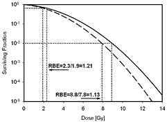
Figure 1. Schematic dose-response curve for photon radiation (solid) and proton radiation (dashed). The RBE at two levels of effect (doses) is indicated.
Download figure:
Standard image High-resolution imageFrom each published experimental data set the following parameters were extracted: αx and βx describing dose-response to photons, α and β describing dose-response to protons, and LETd (dose-averaged LET) at the position of the biological sample. Assuming the same level of effect compared to the reference radiation leads to equation (3), which defines the proton RBE as a function of Dp (proton dose for a single fraction) on the basis of equation (2).

For the case of βx equals 0, it reduces to

As shown in equations (5)–(7), we can also formulate the relationship using RBEmax and RBEmin, i.e. the asymptotic values of RBE at doses of 0 and ∞ Gy, respectively (Carabe-Fernandez et al 2007).


To define proton therapy prescription doses or constraints based on photon treatments, it would be convenient to define the RBE as a function of the photon dose. However, for analyzing proton treatment plans, a definition based on the proton dose is more practical. The data in this review are reported based on the proton dose.
In the framework of the linear-quadratic dose-response formalism, the BED can be defined for proton treatments as shown in equation (8) (Jones and Dale 2000, Carabe-Fernandez et al 2010). Thus, BED considerations are not included in a general RBE definition.

2.1.2. Jejunal crypt regeneration in mice in vivo.
The measurement of jejunum crypt regeneration in mice, i.e. counting the number of regenerated crypts per circumference, has been suggested as a protocol for comparing proton centers. It does represent a clonogenic survival assay. These experiments are typically done at doses between 10 Gy and 20 Gy. One can parameterize the dose-response curves exponentially with free using equation (9).

Accordingly, the RBE relationships for jejunal crypt cells can be deduced leading to equation (10).

2.1.3. Primary endpoints.
Double strand breaks (DSB), chromosome aberrations, mutations, foci formation, micronuclei formation and other primary endpoints are typically fitted following a linear-quadratic relationship given in equation (11).

This leads to the same RBE relationship as for cell survival given in equations (3) and (7).
2.2. Consideration of LET
2.2.1. Dose-averaged LET.
For the purpose of relating RBE values to macroscopic dosimetric parameters, LETd is a reasonable approximation neglecting the track structure, which determines the characteristics of a radiation field. This does not dispute the fact that a cellular or sub-cellular target represents a volume where radiation effects would be more accurately described by microdosimetric quantities such as yD, the dose-averaged lineal energy, or even individual particle tracks. It is clear that LET can not describe the proton track structure with its delta electrons of up to 500 keV energy in detail (Liamsuwan et al 2011). Fortunately, other than for heavy ions, there are many proton tracks crossing a cell for typical therapeutic doses (typically hundreds or thousand of tracks depending on the cell size (Paganetti 2005)) so that neglecting the fine structure and using LET to characterize the radiation field is feasible. Note that at therapeutically relevant doses the number of proton tracks per cell is considerable so that the use of LETd is more appropriate than the use of the track-averaged LET (Grassberger and Paganetti 2011). Figure 2 shows the LETd as a function of proton energy.
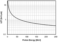
Figure 2. Proton LET as a function of energy for protons traveling through water (Janni 1982).
Download figure:
Standard image High-resolution image2.2.2. Simulation of proton LET for proton experiments.
The majority of published experiments do not provide LETd values at the point of measurement. When those measurements were done as track segment irradiations with a well defined proton energy, the respective LETd were obtained from reference tables (Janni 1982). Many reported proton experiments were done in a radiation therapy treatment facility with a therapeutic beam delivering a spread-out Bragg peak (SOBP) having a specific range (defined for example as the 90% distal dose fall-off) and modulation width (typically defined as the distance between the range and the 90% proximal dose fall-off). In those cases, if LETd values were not reported, Monte Carlo simulations were performed.
The simulation of LETd in water for all experimental data was done using the TOPAS Monte Carlo system (Perl et al 2011). This code has been extensively validated for proton therapy (Testa et al 2013). As a standard feature the code offers a scorer for LETd distributions. A scorer is a function called by the user to record a specific simulation property, e.g. a histogram showing the dose in a certain area. The step size of the protons was limited by the occurrence of a physics interaction or the binning as a function of depth (1 mm). TOPAS has been used previously to simulate LETd distributions in water media as well as patient environments (Grassberger et al 2011, Giantsoudi et al 2013, 2014, Sethi et al 2014). LET distributions can also be calculated analytically (Wilkens and Oelfke 2003) but analytical methods can show significant deviations from accurate Monte Carlo simulations because the latter takes into account secondary particles (Grassberger and Paganetti 2011).
The LETd as a function of position in a SOBP is not fully determined by the range and modulation width of the SOBP. Similar SOBP distributions can be delivered by different proton energy and fluence distributions, i.e. LETd distributions (Paganetti and Schmitz 1996, Paganetti and Goitein 2000, Carabe et al 2012). Because detailed information on all delivery systems used in the published experiments were not reported, it was assumed that these measurements were done at the Francis H Burr Proton Therapy Center at Massachusetts General Hospital for which a very detailed model of the delivery system was available (Paganetti et al 2004). The error in LETd within a SOBP associated with this assumption is probably ~10%. Larger differences between two SOBP showing the same range and modulation width might occur in the distal fall-off because the dose gradient depends on the beam's energy spread.
2.2.3. Clinically relevant range of LET.
Experimental dose-response data are reported for a large range of LETd values. Some of the data involve very low energy protons, i.e. high LETd values. While these data might help to understand biological mechanisms, the direct clinical significance is limited because these protons may only contribute significantly in areas receiving very low doses. The range of LETd values of clinical relevance is shown in figure 3. The LETd distribution in a proton beam depends on the range and modulation width. One can expect that the average LETd across the irradiated volume is lower for a bigger prescribed range because the average proton energy is higher. The difference is however quite small, in particular if the SOBPs are delivered in cyclotron based system where the water equivalent pathlength for each proton is the same independent of the range in the phantom/patient. This could be different for a synchrotron based system.
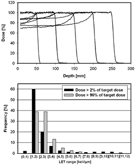
Figure 3. SOBP dose distributions based on a delivery system at the Massachusetts General Hospital and the respective LETd values. The upper graph shows the SOBPs (range/modulation widths: 5 cm/5 cm, 10 cm/5 cm, 10 cm/10 cm, 15 cm/5 cm, 15 cm/10 cm, 20 cm/5 cm, 20 cm/10 cm, 25 cm/5 cm, 25 cm/10 cm). The lower graph shows the distribution of LETd values within bins of 1 keV μm−1 width combined for all SOBPs considering doses higher than 2% of the target dose (black) and considering target regions only (grey; doses within 10% of the SOBP dose plateau). Doses and LET values were scored on the central axis within the homogeneous field area.
Download figure:
Standard image High-resolution imageMore important than the range dependence is the dependence on the modulation width. Because the LETd increases with depth more pronounced towards the end of range, its value in the center of an SOBP increases with decreasing modulation width. As illustrated in figure 3, the average LETd for 4 different SOBPs having a modulation width of 10 cm (ranges of 25 cm, 20 cm, 15 cm, and 10 cm) is ~2.3 keV μm−1, while the 4 SOBPs with the same range but a modulation width of only 5 cm have an average LETd of ~2.85 keV μm−1. In both cases only those areas with a dose bigger than 90% of the average target dose were considered. Note that intensity modulated proton therapy does not necessarily result in an SOBP dose distribution per field, which could influence the LETd distribution significantly.
For the target region close to 80% of the protons have LETd values between 1 keV μm−1 and 3 keV μm−1. In the center of the SOBP, the average LETd is between ~2.8 keV μm−1 and ~2.1 keV μm−1 (decreasing with the depth position of the SOBP center). The maximum expected LETd value in the target (doses >90% of the target dose) turns out to be ~8 keV μm−1 while for the area outside of the target it can go up to ~12 keV μm−1 (for doses >2% of the target dose and the SOBPs considered here). Very small regions at the distal fall-off of the SOBP can show much higher LET values. These numbers are in line with findings in patients (Grassberger and Paganetti 2011). The average value in the center of an SOBP is about 2.5 keV μm−1 as illustrated in figure 4. Note that for low energy beams and small modulation widths (e.g. as used for treating ocular melanoma), LET values could be higher, i.e. potentially up to ~5 keV μm−1 in the SOBP center and ~20 keV μm−1 in the potentially very sharp fall-off.

Figure 4. SOBP depth dose distribution for a field with a range of 15 cm and a modulation width of 10 cm (solid line). The dashed line shows the respective LETd distribution. The shaded areas resemble the center region of the SOBP and the range of LETd, i.e. between ~2.0 keV μm−1 and ~3.0 keV μm−1.
Download figure:
Standard image High-resolution image2.2.4. Reference photon radiation.
RBE values and photon dose-response curves reported in the literature are using different types of reference photon conditions, from mega-voltage to kilo-voltage.
Different photon energies are subject to different LET values (defined via the respective secondary electrons) causing, for example, 250 kVp x-rays to have an RBEx of 1.15 relative to 60Co (Sinclair 1962). When RBE values are calculated using equations (3), (7), or (10), this has to be considered because the photon dose-response curves with their αx and βx refer to the reference radiation used. The reported photon reference radiations that were analyzed included 10 MV photons, 6 MV photons, 4 MV photons, 2 MV photons, 1 MV photons, 60Co, 137Cs, 300 kVp x-rays, 290 kVp x-rays, 250 kVp x-rays, 240 kVp x-rays, 225 kVp x-rays, 220 kVp x-rays, 200 kVp x-rays, 180 kVp x-rays, 130 kVp x-rays, 125 kVp x-rays, 120 kVp x-rays, and 70 kVp x-rays. In very few cases there were only proton data reported but no x-ray data. Such reports were only included in the review if the same group had published x-ray data for the same endpoint measured in the same lab.
As the RBEx for the considered endpoints is typically not known, correcting the RBE values deduced from these experiments based on an average RBEx of the reference radiation is not feasible. Consequently, LETd values were normalized instead. An appropriate reference LETd is the one for 6 MV photons because this is the clinically most relevant radiation source. For those experiments with reference radiations other than 6 MV photons, the proton LETd was corrected according to the difference between the reported reference photons and 6 MV photons based on figure 5. The actual LETd might vary depending on the exact energy spectrum of the source. For cases where 137Cs was used as reference, an LETd of 0.91 keV μm−1 or 0.2 keV μm−1 was assumed depending on the reported procedure.

Figure 5. Dose-averaged LETd of the resulting electrons as a function of the nominal photon energy used for normalizing proton LETd values (Kellerer 2002).
Download figure:
Standard image High-resolution image3. Results
3.1. Proton RBE related to tumor control probability
3.1.1. Clonogenic cell survival.
There is only a small number of in vivo data and a lack of mechanistic knowledge about tumor response to radiation in vivo. Thus, the most relevant endpoint correlated to RBE and TCP is clonogenic cell survival, which is also the most studied endpoint. Nevertheless, there are various pathways leading to cell death, which is not caused by radiation-induced damage itself but a combination of damage and apoptosis or failure to complete mitosis.
This section includes cell survival data not only obtained from tumor cells but also from normal cells, thus assuming that all cell survival data are valuable to determine RBE for tumor response. For this review 76 reports from the open literature were assessed. This includes ~90% of all published data. Some old publications from before 1970 and publications in Russian or Japanese journals were difficult to track down. Further, there are quite a few conference proceeding publications from the mid to late 1960s mostly on whole body effects in experimental animals that could not be retrieved.
Ideally, each of the publications would list αx and βx for the reference x-ray radiation, α and β obtained from the proton survival curve, and the LETd values at the measurement positions to allow data analysis applying equation (3). Some publications do in fact list all of these parameters (Bird et al 1980, Perris et al 1986, Hei et al 1988b, Belli et al 1989, 1990, 1991, 1992a, 1993, 1998, 2000a, Folkard et al 1989, 1996, Bettega et al 1990, 1998, Prise et al 1990, Goodhead et al 1992, Courdi et al 1994, Sgura et al 2000, Green et al 2001, 2002, Baggio et al 2002, Schuff et al 2002, Petrovic et al 2006, 2010, Ristic-Fira et al 2008, Antoccia et al 2009, Ibanez et al 2009, Matsuura et al 2010, Gerelchuluun et al 2011, Wera et al 2011, 2013, Yogo et al 2011, Britten et al 2013, Jeynes et al 2013, Wouters et al 2014, Chaudhary et al 2014, Slonina et al 2014, Keta et al 2014).
It was often necessary to simulate the LETd values assuming that the experiments had been done at our institution, utilizing a detailed geometrical model of the treatment head delivering an SOBP that matched the range and modulation width of the reported SOBP. Some experiments were done with low energy and thus low range proton beams below the range deliverable at our facility (i.e. ~6 cm). In these few cases a pre-absorber upstream of the experimental setup was simulated. A subset of publications listed αx and βx for the reference x-ray radiation as well as the α and β values so that only the LETd had to be simulated based on the beam energy or the information of the range and modulation width of the Bragg curve (Raju et al 1978a, Urano et al 1980, Satoh et al 1986, Blomquist et al 1993, Yashkin et al 1995, Gueulette et al 1996, Coutrakon et al 1997, Tang et al 1997, Matsumura et al 1999, Bettega et al 2000, Ando et al 2001, Schettino et al 2001, Calugaru et al 2011, Kase et al 2013, Matsumoto et al 2014).
Some reports did not mention any of the parameters αx, βx, α, β, or LETd so that the survival curves had to be extracted from the publications and fitted (using matlab (Mathworks Inc.)) in addition to simulating LETd values (Robertson et al 1975, 1994, Hall et al 1978, Williams et al 1978, Raju et al 1978b, Bettega et al 1979, Sakamoto et al 1980, Fuhrman Conti et al 1988, Ogata et al 2005, Kagawa et al 2002, Baek et al 2008, Butterworth 2012, Grosse et al 2014, Zhang et al 2013, Aoki-Nakano 2014). In some incidents the LETd values were reported but the α and β values for all measured conditions as a function of proton energy or position in the Bragg curve had to be manually extracted (Wainson et al 1972, Inada et al 1981, Hei et al 1988a, Wouters et al 1996, Ogheri et al 1997, Moertel et al 2004, Yang et al 2007, Ristic-Fira et al 2011, Doria et al 2012).
In addition to measurements in pristine or spread-out Bragg peak depth dose curves semi-monoenergetic proton beams were used with low energy (<6 MeV) (Bettega et al 1979, 1998, Bird et al 1980, Perris et al 1986, Hei et al 1988a, 1988b, Belli et al 1989, 1992a, 1993, 1998, 2000a, Folkard et al 1989, 1996, Prise et al 1990, Goodhead et al 1992, Ogheri et al 1997, Sgura et al 2000, Schettino et al 2001, Baggio et al 2002, Antoccia et al 2009, Wera et al 2011, 2013, Fiorini et al 2011, Yogo et al 2011, Doria et al 2012, Jeynes et al 2013) and higher energies (>6 MeV) (Wainson et al 1972, Perris et al 1986, Fuhrman Conti et al 1988, Bettega et al 1990, Green et al 2001, 2002, Moertel et al 2004, Yang et al 2007).
For those publications referring to monoenergetic protons, the LETd values could be looked up. Where LETd values were reported we confirmed that these are consistent with published energy-range tables (Janni 1982) (also in one case LETd values were simulated because the reported ones where unreasonably high for the given SOBP (Britten et al 2013)).
Because the goal was to establish relationships between dose, endpoint, and LETd, those publications that reported only single doses or RBE values without dose-response relationships were not included in the analysis (e.g. Biaggi et al 1999, Kajioka et al 2000, Ghosh et al 2010, Elsasser et al 2010, Auer et al 2011, Fu et al 2012). Also not included were split-dose experiments (Antonelli 2001). One experiment did not report on a reference photon experiment (Kanemoto et al 2014) but a related publication (Matsumoto et al 2014) could be used to include part of the data in the analysis.
The experimental data are associated with considerable uncertainties, i.e. statistical uncertainties due to the stochastic nature of radiation effects and due to variations in cell sensitivity within the same culture. There are also systematic uncertainties caused by, for example, laboratory specific handling of cell cultures or dosimetry. The estimation of the true uncertainty in those experiments is difficult. Furthermore, the reporting of uncertainties in the analyzed publications is rather inconsistent and not always did reports include standard deviations or confidence intervals. Uncertainties not only exist for the reported α and β values but also for the LETd values particularly at high LETd (~ >20 keV μm−1) because of difficulties deducing LETd values for such experiments.
Tables A1–A4 in the Appendix list all data on cell survival. Note the same cell type can belong to different strains showing differences in dose response. In most in vitro experiments Chinese hamster cell lines were used, e.g. mostly V79. The key parameters are shown in table A1. In addition, many rat or mouse cell lines have been used as summarized in table A2. A considerable amount of data is also available on human cancer cell lines (table A3) as well as other human cells (table A4). Most publications and experiments in vitro were focusing on cell survival in the dose range between ~1 Gy and ~10 Gy.
RBE as a function of LET.
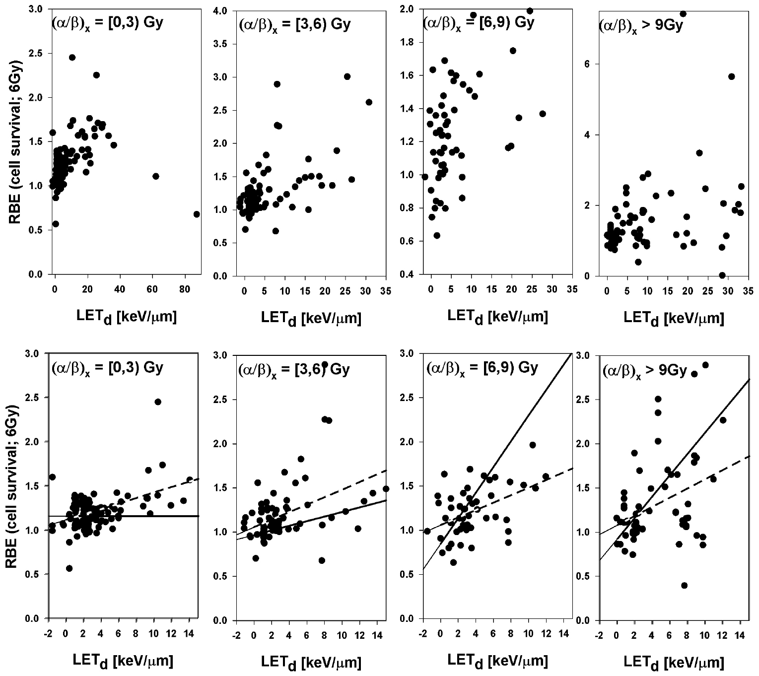
The RBE for cell survival (based on tables A1–A4) is shown as a function of LETd for 4 different bins of (α/β)x in figures 6 and 7 for 2 Gy and 6 Gy, respectively. In the clinically relevant range of LETd one expects a more or less linear behavior of RBE as a function of LETd for a given αx and βx (Wilkens and Oelfke 2004, Tilly et al 2005, Carabe et al 2013, Wedenberg et al 2013). Proton biological effectiveness will eventually decrease with increasing LETd due to overkill effects but this happens at very low proton energies typically irrelevant for clinical considerations. Figure 8 shows all data in one single graph. Linear fits were done for all data sets although the relationship could potentially be not strictly linear with a smaller slope at low LET. The error bars for the reported parameters leading to the RBE are substantial and therefore not shown to avoid obstructing the plots.

Figure 6. RBE for cell survival as a function of LETd at a proton dose of 2 Gy (from left to right: (α/β)x between 0 Gy and 3 Gy, between 3 Gy and 6 Gy, between 6 Gy and 9 Gy, and above 9 Gy). The upper row shows all data points included in the analysis. The lower row includes only data with LETd values ≤15 keV μm−1, the area most clinically relevant. LETd values are given relative to the reference photon radiation. The solid lines are fits through the data included in each plot considering the published uncertainties. The dashed lines show the fit results without considering individual uncertainties.
Download figure:
Standard image High-resolution image
Figure 7. RBE for cell survival as a function of LET at a proton dose of 6 Gy (from left to right: (α/β)x between 0 Gy and 3 Gy, between 3 Gy and 6 Gy, between 6 Gy and 9 Gy, and above 9 Gy). The upper row shows all data points included in the analysis. The lower row includes only data with LETd values ≤15 keV μm−1, the area most clinically relevant. LETd values are given relative to the reference photon radiation. The solid lines are fits through the data included in each plot considering the published uncertainties. The dashed lines show the fit results without considering individual uncertainties.
Download figure:
Standard image High-resolution image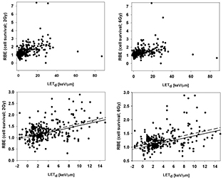
Figure 8. RBE for cell survival as a function of LET at a proton dose of 2 Gy (left) and 6 Gy (right). The upper row shows all data points included in the analysis. The lower row only includes data with LETd ≤15 keV μm−1, the area most clinically relevant. LETd values are given relative to the reference photon radiation. The solid lines are fits through the data included in each plot considering the published uncertainties. The dashed lines show the fit results without considering individual uncertainties.
Download figure:
Standard image High-resolution imageWhen analyzing the published experiments it became apparent that reported uncertainties for key parameters such as α and β are often unrealistic, i.e. over- or underestimated. Therefore, two separate fits were done, one using the reported uncertainties for each data point and one considering all data points with equal weight. This substantially impacts the slope of RBE versus LETd when grouping according to (α/β)x (figures 6 and 7). For all data combined (figure 8) the slope is very similar but the overall RBE is slightly higher if errors bars from each publication are not considered.
All parameters for the linear fits are listed in table A5. As expected, there is a positive slope of RBE as a function of LETd, which decreases with increasing dose. One might expect a steeper slope as (α/β)x decreases. The data do not confirm this, likely due to experimental uncertainties. In fact, when treating each data point equally, the slope is very similar for all four (α/β)x regions. Table 1 shows average RBE values for different LETd bins considering all (α/β)x values. For the fit restricted to clinically relevant LETd values (≤15 keV μm−1), the RBE at the reference photon LETd turns out to be 1.02 ± 0.04 at 2 Gy and 0.99 ± 0.03 at 6 Gy (if given equal weights to all data points, the values are 1.08 ± 0.06 and 1.08 ± 0.05, respectively). This is roughly in line with the common expectation that protons with an LETd equal to the photon reference should show an RBE of 1.0. However, for (α/β)x <3 Gy, the RBE at the reference LETd turns out to be 1.24 ± 0.07 at 2 Gy and 1.15 ± 0.05 at 6 Gy (the numbers are ~1.16 ± 0.07 and ~1.11 ± 0.05, respectively, if all data points are equally weighted). This suggests that at low (α/β)x the RBE for LETd values equal to the reference photon radiation is not 1.0. Differences in energy deposition patterns between photons and protons could potentially cause an RBE ≠ 1.0 even at comparable LET values due to a difference in radiation response mechanisms.
Table 1. Average RBE values based on the data shown in figure 8 considering all (α/β)x. LETd values are given relative to the reference photon radiation. Uncertainties are based on 95% confidence intervals.
| Average RBE (2 Gy) | Average RBE (2 Gy); weights=1 | Average RBE (6 Gy) | Average RBE (6 Gy); weights=1 | |
|---|---|---|---|---|
| LETd = photon LETd (from linear fit with LETd ≤ 15 keV μm−1) | 1.02 (0.98, 1.06) | 1.08 (1.02, 1.14) | 0.99 (0.97, 1.02) | 1.08 (1.03, 1.13) |
| 2 <LETd < 3 keV μm−1 | 1.12 (1.07, 1.16) | 1.18 (1.13, 1.24) | 1.09 (1.07, 1.12) | 1.15 (1.11, 1.19) |
| LETd < 3 keV μm−1 | 1.10 (1.07, 1.13) | 1.15 (1.11, 1.19) | 1.06 (1.04, 1.08) | 1.13 (1.10, 1.15) |
| 3 ≤ LETd < 6 keV μm−1 | 1.21 (1.16, 1.26) | 1.38 (1.28, 1.49) | 1.14 (1.11, 1.18) | 1.33 (1.24, 1.41) |
| 6 ≤ LETd < 9 keV μm−1 | 1.35 (1.25, 1.44) | 1.38 (1.21, 1.55) | 1.27 (1.19, 1.35) | 1.36 (1.18, 1.54) |
| 9 ≤ LETd ≤ 15 keV μm−1 | 1.72 (1.54, 1.89) | 1.74 (1.53, 1.95) | 1.60 (1.36, 1.84) | 1.53 (1.34, 1.72) |
The data clearly show an increase of RBE with increasing LETd. The RBE value of 1.1 was chosen as the basis for today's clinical practice by considering data obtained in the central part of an SOBP. If we assume the LETd in the central region of an SOBP to be typically between ~2.0 keV μm−1 and ~3.0 keV μm−1 (keeping in mind that it could be up to ~5 keV μm−1 for low range fields with small modulation widths), the average RBE is 1.12 ± 0.05 at 2 Gy and 1.09 ± 0.03 at 6 Gy (if given equal weights to the data, the values are 1.18 ± 0.06 and 1.15 ± 0.04, respectively). Thus, the analysis of all available experimental data show an RBE of ~1.15 as an average for the dose plateau in an SOBP, i.e. slightly higher than the currently assumed clinical RBE of 1.1.
Also of interest are RBE values over a range of LETd, i.e. the average RBE for LETd values between 0 keV μm−1 and 3 keV μm−1 (the entrance region of an SOBP up to the SOBP center), between 3 keV μm−1 and 6 keV μm−1 (the downstream half of an SOBP), between 6 keV μm−1 and 9 keV μm−1 (distal edge region), and between 9 keV μm−1 and 15 keV μm−1 (SOBP dose fall-off region). For the entrance region up to the center of the SOBP the average RBE at 2 Gy is 1.10 ± 0.03 (or 1.15 ± 0.04 if equal weights are assumed for all data). For the downstream half of the SOBP the RBE value at 2 Gy increases to 1.21 ± 0.05 (or 1.38 ± 0.11 for equal weights). The distal edge region shows an average RBE values at 2 Gy of 1.35 ± 0.10 (or 1.38 ± 0.17 for equal weights). Finally, for the fall-off one finds 1.72 ± 0.18 (or 1.74 ± 0.21 for equal weights). Note that these averages over all cell lines may not be necessarily representative for clinically relevant tissues. Nevertheless, there is a significant increase of RBE as a function of depth in tissue for an SOBP proton therapy field. The increase is more moderate at 6 Gy as compared to 2 Gy (table 1). Figure 9 shows (independent of (α/β)x) how the RBE at 2 Gy increases with depth for the SOBPs shown in figure 3. The RBE at the distal edge turns out to be about 1.35, on average.

Figure 9. Increase of RBE for 2 Gy (relative to 6-MV photons) across various SOBPs. A: range/modulation widths: 5 cm/5 cm; B: 10 cm/5 cm and 10 cm/10 cm; C: 15 cm/5 cm, 15 cm/10 cm; D: 20 cm/5 cm, 20 cm/10 cm; E: 25 cm/5 cm, 25 cm/10 cm. The RBE values are based on a linear fit of RBE versus LETd in the range of LETd ≤ 15 keV μm−1 independent of (α/β)x (fit parameters from table A5, second row, column 2 and 3). Only the region > 95% of the SOBP dose is shown.
Download figure:
Standard image High-resolution imageThe increase in RBE as a function of depth in an SOBP also impacts the position of the distal dose fall-off. An increasing RBE with depth can lead to a shift in the fall-off (physical dose versus biological dose) of up to 4 mm, depending on dose and (α/β)x (Robertson et al 1975, Carabe et al 2012, Matsumoto et al 2014)
RBE as a function of (α/β)x.
The RBE for cell survival is shown as a function of (α/β)x for 4 different bins of LETd in figures 10 and 11 for 2 Gy and 6 Gy, respectively (data with βx = 0 Gy were excluded). Figure 12 shows all data for LETd ≤ 15 keV μm−1. The error bars for all values are substantial and therefore not shown to avoid obstructing the plots. The fit parameters are listed in table A6 while average RBE values are given in table 2.
Table 2. Average RBE values for different (α/β)x bins. LETd values are given relative to the reference photon radiation. Uncertainty intervals are based on 95% confidence intervals.
| Average RBE (2 Gy) | Average RBE (2 Gy); weights = 1 | Average RBE (6 Gy) | Average RBE (6 Gy); weights = 1 | |
|---|---|---|---|---|
| RBE ((α/β)x <3 Gy, LETd ≤ 15 keV μm−1) | 1.24 (1.21, 1.28) | 1.31 (1.26, 1.36) | 1.15 (1.13, 1.17) | 1.20 (1.17, 1.24) |
| RBE (3 ≤ (α/β)x < 6 Gy, LETd ≤ 15 keV μm−1) | 0.99 (0.95, 1.02) | 1.21 (1.12, 1.29) | 1.01 (0.99, 1.03) | 1.19 (1.11, 1.26) |
| RBE (6 ≤ (α/β)x < 9 Gy, LETd ≤ 15 keV μm−1) | 1.12 (1.03, 1.20) | 1.23 (1.12, 1.35) | 1.02 (0.95, 1.08) | 1.22 (1.13, 1.30) |
| RBE ((α/β)x > 9 Gy, LETd ≤ 15 keV μm−1) | 1.19 (1.11, 1.28) | 1.30 (1.16, 1.43) | 1.12 (1.06, 1.18) | 1.31 (1.19, 1.43) |

Figure 10. RBE for cell survival as a function of (α/β)x at a proton dose of 2 Gy (from left to right: LETd between 0 keV μm−1 and 3 keV μm−1, between 3 keV μm−1 and 6 keV μm−1, between 6 keV μm−1 and 9 keV μm−1, and between 9 keV μm−1 and 15 keV μm−1). The upper row shows all data points included in the analysis. The lower row includes data with (α/β)x below 20 Gy. LETd values are given relative to the reference photon radiation. The solid lines are fits through the data included in each plot considering the published uncertainties. The dashed lines show the fit results not considering the individual uncertainties.
Download figure:
Standard image High-resolution image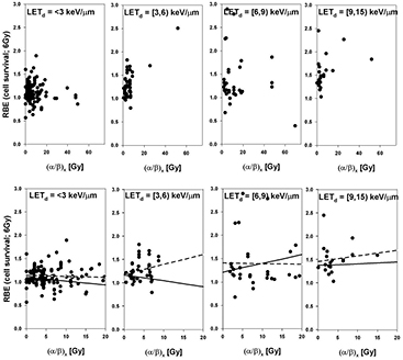
Figure 11. RBE for cell survival as a function of (α/β)x at a proton dose of 6 Gy (from left to right: LETd between 0 keV μm−1 and 3 keV μm−1, between 3 keV μm−1 and 6 keV μm−1, between 6 keV μm−1 and 9 keV μm−1, and between 9 keV μm−1 and 15 keV μm−1). The upper row shows all data points included in the analysis. The lower row includes data with (α/β)x below 20 Gy. LETd values are given relative to the reference photon radiation. The solid lines are fits through the data included in each plot considering the published uncertainties. The dashed lines show the fit results not considering individual uncertainties.
Download figure:
Standard image High-resolution image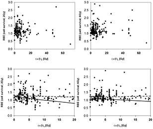
Figure 12. RBE for cell survival as a function of (α/β)x for LETd ≤ 15 keV μm−1 at a proton dose of 2 Gy (left) and 6 Gy (right). The upper row shows all data points included in the analysis. The lower row includes data with (α/β)x below 20 Gy. LETd values are given relative to the reference photon radiation. The solid lines are fits through the data included in each plot considering the published uncertainties. The dashed lines show the fit results not considering individual uncertainties.
Download figure:
Standard image High-resolution imagePrevious studies have indicated that the increase of RBE with decreasing (α/β)x is significant only at low (α/β)x values (below about 5 Gy) (Gerweck and Kozin 1999, Paganetti et al 2000). Also from theoretical considerations one expects an increase of RBE with decreasing (α/β)x (Carabe et al 2012). Surprisingly, the analyzed data do not fully support this, with the exception of the low LETd data (table 2 and figures 10 and 11) although one would expect the slope to be bigger for high LETd values. There is however a small slope at 2 Gy/fraction if all relevant LETd regions are combined (figure 12) and the average RBE at clinically relevant LETd values is highest for (α/β)x <3 Gy (table A5).
RBE as a function of dose.
The dose dependency of the RBE is difficult to assess in the clinically relevant region. Most prescription doses are at ~2 Gy per fraction and thus relevant doses for organs at risk are typically below 2 Gy. However, the majority of experiments have no or at most 1 or 2 data points below 2 Gy. Potential limitations of the linear quadratic model in this region further complicate interpretation of data. Figure 13 shows the dose dependencies for all data from tables A1 to A4. Most experiments predict an increase of RBE as dose decreases, particularly at higher LETd and/or lower (α/β)x. Theoretical considerations suggest a sharper increase in RBE as a function of dose if LETd increases and a sharper increase of RBE as a function of dose with decreasing (α/β)x (Carabe et al 2012). Figure 13 does indicate that for low (α/β)x there might be a more pronounced increase of RBE as dose goes down. It has been speculated that for low-LET radiation the RBE might in fact increase with increasing dose per fraction (Karger et al 2013).

Figure 13. Upper row: RBE for cell survival as a function of dose for different ranges of LETd. Lower row: RBE for cell survival as a function of dose for different ranges of (α/β)x. All figures consider data with (α/β)x < 20 Gy and LETd < 15 keV μm−1. LETd values are relative to the reference photon radiation.
Download figure:
Standard image High-resolution imageRBE modeling.
There are various models to predict RBE values for proton therapy. Summarizing those models is beyond the scope of this review, except for those that apply the same formalism applied in this review (equations (3)–(8)).
For example, Carabe et al applied a linear relationship between RBEmin, RBEmax and LETd depending on (α/β)x resulting in equation (12) (Carabe et al 2012).
The value of 2.686 Gy corresponds to the (α/β)x of V79 cells considered by the authors based on a subset of the data reviewed here. This parameterization can lead to RBE values below 1.0 for high (α/β)x and low LETd. The model predicts an increase in RBE as (α/β)x decreases and assumes a linear increase of α/αx and β/βx with increasing LETd, i.e. it assumes that α and β depend on LETd.
Frese et al (2012) defined α and β as a function of the double strand break yield for the proton radiation, Σ, and the reference radiation, Σx, respectively (equations (13); C is cell type dependent).

In contrast, other approaches assume that β does not change with LETd while considering a linear relationship between α and LETd, as shown in equation (14) (Wilkens and Oelfke 2004). The value of α0 corresponds to a normalization parameter to ensure an RBE of 1.0 at low LETd and depends on αx. Best fits for V79 cells to a limited set of RBE data resulted in α0 = 0.1 Gy−1 and λ = 0.02 μm keV−1 Gy−1 (Wilkens and Oelfke 2004). The same approach was used for RBE based optimization of treatment plans (Frese et al 2011) normalizing to an average RBE of 1.1 in the target and assuming an LETd at the entrance of the proton beam of 0.5 keV μm−1 (equation (15)). An average value for λ of 0.08 μm keV−1 Gy−1 was deduced.


Within the framework of the microdosimetric-kinetic model Hawkins suggested a similar relationship as shown in equation (16) (C is cell dependent) (Hawkins 1998).

Further, the approach by Chen and Ahmad parameterizes the RBE as a function of LETd (assuming a constant β = βx) resulting in equation (17) (Chen and Ahmad 2012). Parameters suggested for V79 cells were α0 = 0.1 Gy−1, λ1 = 0.0013 (keV/μm)−2 and λ2 = 0.045 (keV/μm)−1 Gy.

The approach by Wedenberg et al also assumes no dependency of β on LETd (Wedenberg et al 2013). The reported parameterization for α/αx is shown in equation (18). The best fit value for q was reported as 0.434 ± 0.7 Gy μm/keV using 10 different cell lines.

Finally, Tilly et al (2005) assumed that α/αx linearly increases with LETd and that the slope increases with decreasing (α/β)x with no dependency of β on LETd. The authors assumed different slopes for RBE versus LET for two different (α/β)x (2 Gy and 10 Gy).
The parameterizations in these modeling approaches are based on a small subset of the data reviewed in this work. Most of them assume β = βx, which has the advantage that it allows the RBE to be calculated as a function of LETd and (α/β)x without the explicit knowledge of αx and βx.
Figure 14 shows α/αx, and β/βx as a function of absolute LETd based on this review. Excluded where data with αx ≈ 0 and/or βx ≈ 0. The fit parameters are shown in table A7. If individual error bars are not considered, the dependency of α/αx on LETd is stronger and the slope of α/αx as a function of LETd depends on (α/β)x (figure 14(b)) with lower (α/β)x showing a slightly steeper increase of α/αx with LETd. Also, α/αx (RBEmax) increases with decreasing (α/β)x suspecting that the RBE does in fact increase with decreasing (α/β)x although the data at 2 Gy (see section 'RBE as a function of (α/β)x') were too noisy to show this. No clear dependency on (α/β)x can be established for β/βx as the fits do not show a significant slope (see table A7). An increase in √(β/βx), i.e. RBEmin, as a function of LETd might be visible for LETd values in excess of ~5 keV μm−1, which could potentially be an artifact due to the wider spread of data in this region (figure 14(c)).

Figure 14. Linear quadratic model parameters as a function of absolute LETd for LETd ≤ 15 keV μm−1 and fits through the data. (a): α/αx (i.e. RBEmax), fits include reported uncertainties; (b): α/αx, fits equally weighting all data; (c): β/βx; (d): √(β/βx) (i.e. RBEmin). The linear fits refer to specific ranges of (α/β)x (solid: all (α/β)x; long dashed: (α/β)x < 3 Gy; medium dashed: 3 Gy < (α/β)x < 6 Gy; short dashed: 6 Gy < (α/β)x < 9 Gy; dotted: (α/β)x > 9 Gy). Excluded where data with αx ≈ 0 and/or βx ≈ 0.
Download figure:
Standard image High-resolution image3.1.2. Intestinal crypt regeneration assay in mice.
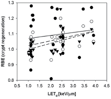
The intestinal crypt regeneration assay in mice is related to the number of surviving cells and was analyzed in several publications (Gueulette et al 1996, 1997, 2000, 2001, 2005, Tepper et al 1977, Ando et al 2001, Kagawa et al 2002, Mason et al 2007, Uzawa et al 2007, Kim et al 2011). This assay can only be used at doses sufficiently high to diminish cell survival so that individual surviving stem cells can be counted. The dose-response curve has three regions, a plateau where according to Poisson statistics all crypts contain at least one surviving cell, a transition region, and an exponential region when most of the regenerated crypts result from the proliferation of a single surviving cell. Analysis is typically done in the dose range between 10 Gy and 20 Gy. No dose dependency down to typical fractionation doses can thus be established. The functional relationship given in equation (10) was used resulting in figure 15 and revealing an increase of RBE with LETd. and an increase of the RBE for decreasing dose. None of the publications included LETd values, so that it was necessary to simulate those. The RBE values are in general between 1.0 and 1.1 (based on linear fits through the data).
Figure 15. RBE for crypt regeneration in mice as a function of LETd. Closed circles and solid line: 10 Gy; open circles and dashed line: 15 Gy; closed triangles and short dashed line: 20 Gy.
Download figure:
Standard image High-resolution image
3.1.3. Tumor response in vivo.
There are methods to directly measure the response of human tumors to radiation. Clinically very relevant are measurements of TCD50, i.e. the dose for 50% local control of the tumor. Human tumor cells that have been irradiated can be implanted in immune-deficient animals in vivo. Subsequently, there is the potential to measure tumor growth in these xenografts, i.e. tumor regrowth after initial shrinkage post radiation. The proton RBE after tumor growth delay of NFSa (fibrosarcoma) in mice has been studied, finding an RBE of ~0.8 (at ~30 Gy relative to 180 kVp x-rays) (Satoh et al 1986). The study of tumor growth delay of human hypopharyngeal squamous cell carcinoma cells in mice resulted in an RBE between 1.1 and 1.2 at ~20 Gy relative to 6 MV photons using a 23 MeV proton beam (Zlobinskaya et al 2014). A study on the recurrence of mouse mammary carcinoma in mice resulted in an RBE of ~1.1 (at ~50 Gy relative to 60Co) (Urano et al 1984). Similarly cell survival can be measured as a surrogate for tumor response by transferring tumor cells to recipient animal or tissue culture, e.g. in the lung colony assay.
It has been hypothesized that cancer stem cells might be more resistant to photon therapy as compared to proton therapy (Fu et al 2012, Zhang et al 2013). Thus, if cancer stem cells have higher resistance compared to non-stem cancer cells, proton irradiation may have greater capability of eliminating cancer stem cells. It has been speculated that this might be due to differences in the production of reactive oxygen species (ROS) (Zhang et al 2013).
Cell migration was studied in human fibrosarcoma cells (Ogata et al 2005) and human non-small cell lung cancer cell lines (Zhang et al 2013) showing a difference between photons and protons. Girdhani et al demonstrated that proton irradiation suppresses cell invasion compared to photon irradiation (Girdhani et al 2012).
Even though it has been shown that in vitro results can correlate with clinical endpoints (Girinsky et al 1993, Gerweck et al 1994), the response in vivo is expected to vary from in vitro response because of the impact of the tumor environment and vasculature on dose response, which could potentially differ between photon and proton irradiation. Angiogenesis is affected by the differences between proton and photon energy depositions. It has been shown that proton irradiation can inhibit angiogenesis (Jang et al 2008, Girdhani et al 2012). Low LET protons (with a proton energy of 1 GeV) do show different levels of pro-angiogenic proteins compared to (low LET) photons (Girdhani et al 2012). This suggests that LET is not the only relevant parameter. In vivo and in vitro response to radiation might differ also because of cell shape and architecture differences, e.g. 3D cell structures might show increased levels of heterochromatin compared to 2D structures affecting double-strand breaks and cell survival (Storch et al 2010).
3.1.4. Other endpoints.
There are various other endpoints that can provide insight into tumor RBE values, such as foci formation, chromosome aberrations or apoptosis (although the latter plays only a minor role in solid tumors). These are discussed below because their relevance for quantifying normal tissue response might be higher than for tumor response, where cell kill is the most important effect. The complexity of these endpoints allow limited quantitative insight into proton RBE for TCP but many of them are relevant to understand TCP as well as NTCP mechanisms.
3.2. Proton RBE related to normal tissue complication probability
3.2.1. Validity of cell survival data.
While cell survival might be the most relevant effect for TCP considerations, other endpoints could potentially be more relevant for NTCP. Organ specific effects of interest are early effects such as erythema and late effects such as lung fibrosis, lung function, or spinal cord injury. It is unlikely that cell survival data can fully describe these. Studies have demonstrated no association between fibroblast radiosensitivity and the development of late normal tissue effects such as fibrosis (Russell et al 1998, Peacock et al 2000). The relationship between clinically observed late effects and DNA repair capacity has been discussed by Bentzen (2006). Surviving cells with unrepaired or misrepaired damage can transmit changes to descendent cells. Malignant transformation can thus be initiated by gene mutation or chromosome aberration
The following sections look at endpoints other than cell survival with respect to proton RBE. As cell survival data for normal cells were included in the section on TCP above, this section also considers endpoints relevant to NTCP that were assessed in tumor cells. While the multitude of effects complicates the definition of a variable RBE, the slope of the NTCP dose response curve is generally steeper compared to TCP dose response curves. Thus, RBE uncertainties could be even more significant, specifically if the dose constraint is close to the tolerance limit. On the other hand, NTCP values are typically small and in a region of a shallow dose-response curve.
3.2.2. Reactive oxygen species.
In the presence of oxygen radiation creates reactive oxygen species (ROS). These ROS lead to oxidative stress and regulate a variety of response pathways. The induction of ROS preceding DNA damage as an indicator of radiation effects on cellular processes was studied in neural precursor cells derived from rat hippocampus. It was shown that the increase of ROS was more rapid with protons compared to photon radiation (Giedzinski et al 2005). The impact of ROS when using proton radiation was also studied using various tumor cells, e.g. lung carcinoma and leukemia (Di Pietro et al 2006, Lee et al 2008a, 2008b, Baluchamy et al 2010, 2012). Differences between protons and photons were not assessed in detail.
3.2.3. DNA strand breaks.
Radiation typically causes thousands of ionization events directly per cell nucleus per Gy. The pattern and frequency does depend on LET, with low-LET radiation causing ionizations that are more homogeneously distributed throughout the cell. Energy deposition by charged particle tracks results in radiation damage in the form of single (SSB) or double strand breaks (DSB), the former are typically repaired efficiently and quickly. Green et al (2001) compared proton and photon induced DNA damage not distinguishing between SSB and DSB. They found an RBE of ~1.2 at 7 Gy at 1 h post irradiation. Studies on the initial yield of DNA DSB in V79 cells showed no significant differences between photon and proton irradiation and weak dependence on LET (Prise et al 1990, Jenner et al 1992, Belli et al 1994, 2000b). Similarly, no difference in initial DSB was reported for human tumor glioblastoma and mammalian fibroblasts (Moertel et al 2004). Barendsen showed that the increase of RBE with increasing LET is less steep for DSB induction than for cell survival (Barendsen 1979). Excess DSB for protons compared to photons was reported for SQ20B cells derived from human epithelium tumors of the larynx and HeLa (human cervix carcinoma) cells, but there was no increase with LET across an SOBP (Calugaru et al 2011). A difference in DSB induction was seen at very high proton LET values (28.5 keV μm−1) in normal human fibroblasts but remarkably no significant difference with LET using various ions was seen (Esposito et al 2006). Further, for very low-LET protons (1 GeV protons with an LET of ~0.22 keV μm−1) a larger yield in DSB was seen compared to 100 kVp x-rays and 137Cs in bacteriophage T7 DNA (Hada and Sutherland 2006). Using plasmid DNA, the same effect was seen by others, i.e. a larger DSB induction for very low-LET protons but comparable yields between protons and photons at medium proton LET values (~3 keV μm−1) (Leloup et al 2005).
In contrast to DSB induction, one would expect a difference between photon and proton irradiation in terms of residual DSBs because the type of DNA damage and thus the repair pathway is expected to differ (Grosse et al 2014). The typical repair mechanism for DSBs in mammalian cells exposed to photons is non-homologous end-joining although homologous recombination might play a bigger role in the late S and G2 phases of the cell cycle. A difference in DNA damage complexity might lead to preferential homologous recombination after proton irradiation (Grosse et al 2014)
There can be differences in complex damage between photon and proton radiation without necessarily increasing the number of measured DSB (Ibanez et al 2009, Grosse et al 2014). Multiple lesions formed within one or two helical turns of the DNA (potentially by a single track) are considered clustered damage (due to clustered energy deposition events) whereas additional lesions close to a DSB are typically referred to as complex damage. Thus, clustered damage can cause damage complexity. Lesion complexity does play a role with respect to cellular repair capacity (Green et al 2001, Pastwa et al 2003, Hada and Sutherland 2006, Georgakilas et al 2013). If lesions are in close proximity they may not be repaired although they might be non-lethal if isolated, e.g. multiple lesions in close proximity on the same or opposing DNA strands are more difficult to repair (Pastwa et al 2003). Measuring residual yields of DSB does in fact show significantly higher values for protons compared to photons (Belli et al 2000b, Moertel et al 2004), e.g. an RBE of 1.8 ± 0.4 at 2 h post irradiation for 11 keV μm−1 protons compared to 60Co (Belli et al 2000b). There are also clustered lesions other than DSB that could result in DSB after failed repair mechanisms (Wallace 1998). Also studied was Olive Tail Moment to assess DNA damage (Joseph et al 2012).
Because the geometrical distribution of the initial damage differs between photons and protons because of different track structures (Liamsuwan et al 2011) the chromatin structure may play a role as well. On the one hand, there may be fewer stand breaks in densely packed chromatin because there is a lower probability of water-moderated radicals. On the other hand, a more densely packed chromatin structure increases the likelihood of closely located sub-lethal lesions. It has been suggested that the radiosensitivity of tumor clonogens can be quantified by measuring the chromatin condensation (Chapman 2003). This demonstrates the importance of understanding energy deposition characteristics when comparing photon and proton radiation.
Note that damage in non-DNA targets in the cell membrane can play a role in cellular responses as well (Prise et al 2005).
3.2.4. Foci formation, repair proteins, and gene expression.
The induction of DSB is often quantified experimentally by studying formation of foci, aggregates of DNA repair-related proteins at the site of DNA strand breaks. Damage to the DNA is identified via protein sensors followed by damage signaling processes including formation of foci and finally damage repair. Because foci formation is related to the type of damage and repair processes used, it is in principle a good measure to assess the energy deposition pattern of different modalities. The number of foci formed initially might be related to the number of DSB (Rothkamm and Loebrich 2003). Specifically the presence of γ-H2AX is a sensitive measure of DSB induction and repair as γ-H2AX molecules are grouped in foci close to the damaged site. Molecules commonly studied for comparison of proton and photon radiation include γ-H2AX (an early indicator of cellular response) and 53BP1 (tumor suppressor p53 binding protein 1). The counting of foci can be challenging and experiments are mostly done at doses in excess of 2 Gy, particularly if assays are done after time for repair has been allowed.
Reported were experiments comparing protons and photons on γ-H2AX foci and 53BP1 foci formation as indicators for DSB in blood lymphocytes (Sorokina et al 2013), foci formation in HeLa cells (Zlobinskaya et al 2012), and 53BP1 foci formation in human umbilical vein cells (Grabham et al 2012). Other studies focused on the difference of protons and photons for the formation of γ-H2AX foci, e.g. after irradiation of HFFF2 fibroblasts (Antoccia et al 2009) or Chinese hamster ovary cells (Grosse et al 2014). Foci formation was also studied using human tumor cell lines MOLT4 (leukemia) and human tumor ONS76 cell lines as surrogate for DSB (Gerelchuluun et al 2011), in human A549 NSCLC adenocarcinoma cells (Wera et al 2013), non-small cell cancer cell lines (Fu et al 2012, Zhang et al 2013), human salivary gland tumor cells (HSG) (Baek et al 2008), and in mouse melanoma cell line (B16-F0) (Ibanez et al 2009).
It was found that the amount of γ-H2AX foci in human salivary gland tumor cells (HSG) did not increase as a function of depth in an SOBP (Baek et al 2008). This is an indication that with increasing LET it is the complexity of damage and not necessarily the number of DSB that determines an increase of the RBE.
The number of foci might be of limited value for defining RBE because it is time dependent as they are surrogates to both damage induction as well as damage repair. The impact of homologous recombination and non-homologous end joining when comparing proton and photon induced DSB has been studied after irradiation of Chinese hamster ovary cells showing that there was no difference in number of γ-H2AX foci between protons and photons at an early time point but the number of foci was different at later time points in an homologous rejoining deficient cell line (Grosse et al 2014). Others have found that the foci formation does differ between protons and photons 30 min after irradiation but that the difference was insignificant after 6 h (Gerelchuluun et al 2011). What does complicate the interpretation of these data is that proton-induced foci can have a different size (Desai et al 2005, Costes et al 2006, Leatherbarrow et al 2006, Ibanez et al 2009, Gerelchuluun et al 2011). Foci typically increase in size as a function of time post radiation. Interestingly, a correlation between the size of foci and cell survival was reported at 6 h post irradiation indicating that the size of foci better correlates with radiation effectiveness compared to the number of foci (Ibanez et al 2009).
In addition, γ-H2AX foci formation and the gene expression patterns after whole body irradiation of mice was assessed (Finnberg et al 2008). Another study looked at gene expression and foci formation in A549 lung adenocarcinoma cells (Ghosh et al 2010). All studies show RBE values of ~1.0 or slightly higher.
Proton and photon irradiation cause different epigenetic responses (Finnberg et al 2008, Goetz et al 2011, Girdhani et al 2013) and most likely regulate genes controlling DNA damage response differently (Finnberg et al 2008, Tian et al 2011, Girdhani et al 2012). Dissimilarities in regulatory proteins between proton and photon irradiation have been demonstrated for lung cancer with respect to inflammatory endpoints (Gridley et al 2004). Similar effects have also been shown in several animal models (Finnberg et al 2008, Rithidech et al 2010). The role of the p53 protein in differences between proton and photon response was studied in human colorectal cells (Baggio et al 2002). Further, gene expression of TP53 (which encodes p53) and CDKN1A was studied in HFFF2 fibroblasts (Antoccia et al 2009). Gridley et al did a genetic analysis of proton radiation effects using human lung epithelial cells in a clinical SOBP beam, albeit without comparing to photons (Gridley et al 2014).
There are two reports on oncogenic transformation at therapeutic doses, one comparing 4.3 MeV protons with alpha particles (Bettega et al 1990) and one reporting an RBE of 1.09 for oncogenic transformation at the level of 0.02% transformants/surviving cell (Hei et al 1988b).
3.2.5. Chromosome aberrations.
Chromosome aberrations are signs of improper repair of DNA damage and are the cause of most mutations. They can activate molecular pathways that result in gene expressions leading to, for example, carcinogenesis (Knudson 2001). The yield and complexity of chromosome aberrations is time dependent due to repair effects and the removal of non-surviving cells from the sample. There is a strong correlation with cell survival.
Data on chromosome aberrations include chromosome aberrations in root tips (Larsson and Kihlman 1960) and chromosome aberrations in human peripheral blood lymphocytes (Todorov et al 1972, Takatsuji et al 1983, Edwards et al 1985, 1986, Matsubara et al 1990, Rimpl et al 1990, Schmid et al 1997, Wu et al 1997, Mognato et al 2003, Govorun et al 2006). Higher aberration frequencies were reported for protons. The RBE values obtained range between ~1.0 and ~1.2 for doses up to ~5 Gy. Significantly higher RBE values were reported in studies using low energy protons (Schmid et al 1997, Mognato et al 2003) while others reported RBE values below 1.0 for lower LET values (Todorov et al 1972). For inter-chromosome exchanges in human fibroblasts the RBE was reported as <1.0 as well (0.4 keV μm−1 protons relative to 137Cs) (Wu et al 1997). Chromosome aberrations in HeLa and Chinese hamster B-11 cells resulted in an RBE of 2 relative to 137Cs in a clinical beam (Wainson et al 1972). Chromosme aberration (dicentrics) in Chinese Hamster hybrid cells were also investigated (Schmid et al 2011). The RBE values relative to 70 kV photons at ~3 Gy were between 0.73 and 0.93.
Some publications did not report a dose dependency (Grosse et al 2014; Schmid et al 2012) or considered only doses in excess of therapeutic dose levels (Hase et al 1999). One study on chromosome aberrations in EUE cells did not report results for a photon reference radiation (Bettega et al 1981).
3.2.6. Mutations and micronuclei formation.
Micronuclei represent loss of genetic material due to chromosome fragments that cannot attach to the mitotic spindle when cells are completing mitosis, i.e. micronuclei are not included into the nuclei of daughter cells. The formation of micronuclei has been assessed in circulating lymphocytes as well as cell lines in culture. One might expect that micronuclei correlate well with loss of clonogenic cell survival because cells with micronuclei do not form colonies. This is different in the case of mutations where cells do have to survive in order to express mutations. Experiments often only consider doses up to 2–6 Gy.
Studying micronucleus formation in cultured human EUE cells showed an RBE of 2.4 (versus 60Co) for 1.8 keV μm−1 protons (Fuhrman Conti et al 1988). A significantly increased effectiveness of protons for micronuclei formation was seen in Fischer rat thyroid follicular cells (Green et al 2001) and in HFFF2 human fibroblasts (Antoccia et al 2009). In contrast, assessing micronucleus formation in C1-1 hamster cells, it was found that the RBE for 7.7 keV μm−1 protons was <1.0 and only increased (to values >2.4) for very high LET protons of 27.6 keV μm−1 (versus 137Cs) (Sgura et al 2000). Differences between proton and photon induced micronuclei were identified in human fibroblasts (Sgura et al 2001). An RBE of about 1.1 relative to 70 kVp x-rays was reported for micronuclei induction in HeLa cells using 20 MeV protons (Schmid et al 2009), which was later confirmed using a human skin model (Schmid et al 2010). A study of human lymphocytes showed an RBE >1.0 for formation of dicentrics but below 1.0 for micronuclei formation (relative to 300 kVp x-rays) (Joksic et al 2000). Micronucleus formation for protons and photons was also studied in AG01522 diploid human fibroblasts (Yang et al 2007). One study did not assess a dose dependency (Schmid et al 2012).
There are reports on HPRT- mutation using V79 cells using very low proton energies (Belli et al 1990, 1991, 1992b, 1993, 1998). The RBE values for mutation were higher than the one for cell survival. This has also been seen at clinically relevant LET values. An RBE of 1.3 was reported for 10 keV μm−1 protons (relative to 4 MV photons) for HPRT mutation in primary human fibroblasts (Hei et al 1988a).
3.2.7. Apoptosis and cell cycle effects.
There are clearly differences in radiation-induced cell cycle perturbations comparing protons and photons. Cell cycle perturbations were studied for human glioblastoma cells (Moertel et al 2004) as well as HFFF2 fibroblasts (Antoccia et al 2002, 2009). Cell cycle phase redistribution, proliferation, and the level of apoptosis in human melanoma cells HTB140 (Petrovic et al 2006, 2010, Ristic-Fira et al 2007, 2011, Todorovic et al 2008, Keta et al 2014) and human ovarian cancer cells (Keta et al 2014) was also studied in one laboratory as well as cell growth, cell cycle redistribution and apoptosis in human melanoma HTB63 cells (Ristic-Fira et al 2001, 2004). Differences in apoptosis between photons and protons were studied for cell lines derived from a bone metastasis of a prostate adenocarcinoma (PC3), from a mammary adenocarcinoma (MCF7), for non-small cell cancer cell lines (Fu et al 2012, Zhang et al 2013), and for cells isolated from a papillomatous carcinoma of the thyroid (Ca301D) (Di Pietro et al 2006). Green et al (2001) looked at apoptosis and cell cycle phase redistribution in Fischer rat thyroid follicular cells. Investigators also looked at cell cycle disruption and time sequence of apoptosis. It appears that protons cause a more immediate entry into apoptosis, possibly due to a different type of damage compared to photons (Green et al 2001). The induction of apoptosis comparing photons and protons was studied for Lewis lung carcinoma cells (LLC), HepG2 human hepatocellular carcinoma cells and Molt-4 human leukemia cells (Lee et al 2008a, 2008b). Other data include DNA synthesis and apoptosis in human A549 alveolar adenocarcinoma cells (Wera et al 2013), HTB140 (Ristic-Fira et al 2008), and MOLT4 human leukemia cell lines (Gerelchuluun et al 2011). DNA synthesis differences as a function of dose were also studied for V79 cells (Matsumura et al 1999). These studies show an increased level of apoptosis after proton compared to photon radiation. No significant difference was seen in T-lymphocytes (Radojcic and Crompton 2001).
Additionally, organ specific differences in apoptotic response after whole-body irradiation of mice (Finnberg et al 2008) or neural activity suppression in frog static nerves (Gaffey 1971) were assessed.
Differences in the apoptotic pathways when comparing both modalities can shed light on the underlying mechanisms of radiation effects (Di Pietro et al 2006, Finnberg et al 2008, Baluchamy et al 2010, 2012, Girdhani et al 2013)
3.2.8. In-vivo animal models.
Many endpoints have been studied in animal models, such as skin reactions, organ weight loss or LD50 (dose at which half the laboratory animals die). The majority of these experiments are in line with an RBE of about 1.1 relative to 60Co. Specifically, reports considered mortality and hematological or cardiovascular changes in primates after whole body radiation (LD50) (Kundel 1966, Dalrymple et al 1966a, 1966b, 1966c, Taketa et al 1967, Zellmer et al 1967), mice mortality after whole body irradiation (LD50) (Tobias et al 1952, Bradley et al 1964, Baarli and Bonet-Maury 1965, Dalrymple et al 1966d, Ashikawa et al 1967, Jesseph et al 1968) or thorax irradiation (LD50) (Stenson 1969b, Urano et al 1984, Gueulette et al 2000), as well as tumor induction and life shortening after whole body irradiation in mice (Clapp et al 1974). Some of these whole-body experiments were mainly done for space radiation research. They consistently show RBE values between ~1.0 and ~1.3. Also reported were endpoints such as late effects on rat rectum (Stenson 1969a) and chorioretinal edema in owl monkey eyes (Constable et al 1976). Studies on cataract formation or lens opacities in mouse lenses (Darden et al 1970, Urano et al 1984), length of tail vertebrae in mice (Urano et al 1984), testes weight loss in mice (Baarli and Bonet-Maury 1965, Urano et al 1984), weight loss in other organs in mice (Warshaw and Oldfield 1957, Baarli and Bonet-Maury 1965, Montour et al 1969), and blood count after whole body irradiation in mice (Kajioka et al 2000) resulted in RBE values typically between ~1.0 and ~1.3. The RBE for lens opacity in rabbit lenses was measured to be between 2 and 2.6 versus 1 MV photons (Cleary et al 1972, 1973). Studied by several groups were acute skin reactions in mice (Tepper et al 1977, Raju and Carpenter 1978, Satoh et al 1986, Tatsuzaki et al 1987, 1991, Nemoto et al 1998) and rabbits (Falkmer et al 1959) as well as late feet deformity in mice (Raju and Carpenter 1978). These data show RBE values for skin reaction typically in the range of 1.1–1.25, with the exception of two studies showing RBE values between 0.8 and 0.9 (relative to 290 kVp x-rays) (Tatsuzaki et al 1987, 1991). Some animal data did not include photon data for reference (Lindsay et al 1966, Krupp 1976, Yochmowitz et al 1985, Dalrymple et al 1994). The genetic damage in spermatological stem cells was studied after whole body irradiation of mice and rats with a comparison between low-LET protons and photons (Vaglenov et al 2007). To establish RBE values for all relevant in vivo endpoints would require a tremendous effort and a considerable number of animals.
3.2.9. Other endpoints.
There are quite a few experiments using relatively low doses (because the focus was on space radiation effects), e.g. on chromosome aberrations in human lymphocytes up to 0.7 Gy (George et al 2002). On the other hand, there were also survival data reported on Lewis lung carcinoma cells (LLC), HepG2 human hepatocellular carcinoma cells and Molt-4 human leukemia cells that used extremely high doses (up to 100 Gy) where the resolution in the region of interest is too coarse to be of relevance for clinical purposes (Lee et al 2008b). For the same reason studies on DSB induction in human cells and V79 cells for dose ranges between 25 Gy and 250 Gy (Belli et al 2001, 2002, Campa et al 2005) and for DSB induction in human skin fibroblasts in the dose range of 100–600 Gy (Frankenberg et al 1999) are of limited value for defining a clinical RBE.
Effects not directly related to DNA damage may play a role as well, such as bystander effects, genomic instability, and abscopal effects. Considerable differences between photon and proton irradiation might exist but are not well understood (Schmid and Multhoff 2012). The actual geometry and density of sub-cellular structures such as chromatin might impact the biological effect as a function of energy deposition characteristics as well (Storch et al 2010, Santos et al 2013).
4. Discussion
For the purpose of defining clinical RBE values only experimental data on clonogenic cell survival are available in large quantities. Thus, RBE values currently can be defined only based on these data (albeit with still large uncertainties). This may be sufficient for TCP considerations and for some normal tissue effects.
For NTCP, the variety of endpoints other than cell survival and the large spread of results do currently not allow a comprehensive analysis towards a clinical RBE. Going forward, the most promising endpoint for understanding RBE related to NTCP might be the induction of inflammatory molecules such as cytokines after radiation. Examples are the Tumor Necrosis Factor (TNF-α), which regulates inflammation in tissue or the Transforming Growth Factor (TGF-β). Both are related to pneumonitis and fibrosis. Another example is Interleukin-6 (IL-6), a cytokine regulating the immune system defense to tissue damage. However, the relationship to any given tissue response is complicated as various cytokines are usually involved and there may be complex relationships between the cytokines varying with time after irradiation. Measuring RBE using these endpoints is currently elusive.
For organs at risk the concept of RBE might be fundamentally flawed and is only a surrogate for other effects potentially not understood in detail. When proton dose distributions are related to photon dose distributions by applying an RBE we are not really normalizing proton dose (and outcome) to photons. Proton dose distributions in critical structures are typically more heterogeneous compared to photon therapy. Yet most dose constraints are defined based on mean dose. The RBE values extracted from cell experiments are valid for homogeneous doses and would thus need to be applied on a voxel-by-voxel basis if used clinically. The definition of RBE for NTCP requires a voxel-by-voxel analysis with potentially defining a concept like the equivalent uniform biological dose similar to the equivalent uniform dose concept (Niemierko 1999). This holds not only for applying variable RBE values but also when analyzing treatment outcomes with respect o potential RBE variations (Sethi et al 2014, Giantsoudi et al 2014).
The difference in dose distribution between proton and photon therapy could have even more complex consequences, e.g. when interpreting side effects we might have to investigate physiological interactions of different organs (e.g. lung and heart) (van Luijk et al 2007, Paganetti and van Luijk 2013).
Finally, inter-patient variability in radiosensitivity could be similar or even larger than general RBE variations. Genomic or functional biomarkers to define individual radiosensitivity or to group patient populations are thus clearly desirable (Liu et al 2014).
5. Summary and conclusion
For this review 369 data points from 76 publications were considered to estimate the RBE for cell survival. Additionally, about 100 reports on endpoints other than cell survival were assessed. The basic findings are as follows:
- Given the large amount of data it is surprising that the RBE for clinically relevant LETd values, (α/β)x values and doses is still associated with considerable uncertainties.
- Despite the abundant in vitro and in vivo evidence supporting the notion that RBE depends on many factors, the use of a generic clinical RBE of 1.1 at 2 Gy does not seem unreasonable if an average for an SOBP field is assigned (although the data show a slightly higher average of ~1.15). Caution is warranted for small modulation widths and/or low (α/β)x where the average RBE could be higher. Note that, if a generic value is to be used, it should be chosen conservatively to ensure tumor prescription doses.
- The RBE increases with increasing LETd and thus with increasing depth if a SOBP is being delivered. The RBE is significantly higher towards the distal end of an SOBP. For a typical spread-out Bragg peak delivery and averaged over all (α/β)x, the average RBE does increase with depth from ~1.1 in the entrance region, to ~1.15 in the center, ~1.35 at the distal edge and ~1.7 in the distal fall-off. The values for 6 Gy are significantly lower. For low energy beams and small modulation widths, LETd and thus RBE values can be higher.
- There is a trend of an increase in RBE as (α/β)x decreases but this trend is not as apparent as one might have expected. The current clinical RBE could potentially underestimate the RBE at low (α/β)x and overestimate the RBE at high (α/β)x.
- RBE for cell survival seems in general to increase with decreasing dose, particularly for high LETd or low (α/β)x.
- The relevance of various reported endpoints other than cell survival for defining clinical RBE values for NTCP is unclear at this time. In general, RBE values for endpoints other than clonogenic cell survival are not in disagreement with a clinical RBE of 1.1. On the other hand, selected endpoints do show considerable deviations from this value.
The analysis of most of the reported data was difficult for various reasons. Only a subset of the publication provided complete information. Many did not include information on the underlying physics (i.e. LETd) and many did not report the linear-quadratic model parameters. In addition, information on the used uncertainty analysis was often missing. Given the amount of published data for clonogenic survival the substantial spread of the results is remarkable and it is therefore hard to believe that more measurements will reduce uncertainties to a clinically acceptable level. Standardization of the experimental procedures and the error reporting is desirable. The wide spread of data is not solely caused by uncertainties in the experiments but also by variations within the same cell strain.
Clinical data could be analyzed to better understand proton RBE values, at least for different tumors. For organs at risk this is hampered by differences in organ dose distributions between modalities. Patient variability might be significant as well. Variations in RBE could impact the analysis of clinical trials comparing proton and photon treatments. Thus, considering (α/β)x as well as estimating LETd in regions of interest, or even on a voxel-by-voxel bases, is recommended.
Acknowledgments
The author would like to thank Drs Kathy Held and Clemens Grassberger for reading parts of the manuscript and providing valuable comments and suggestions.
Appendix
Table A1. Reported dose response data for clonogenic cell survival using Chinese Hamster cell lines in vitro (A: Chinese Hamster Lung Fibroblasts V79; B: Chinese hamster lung fibroblasts V79-WNRE; C: Chinese hamster lung fibroblasts V79-379A; D: Chinese hamster lung fibroblasts V79/753B; E: Chinese hamster lung fibroblasts V79-4; F: Chinese hamster ovary; G: Chinese hamster ovary AA8; H: CH clone 431; I: Chinese hamster B-11; J: Chinese hamster lung C1-1; K: B14 Hamster fibroblasts). Data sorted by (α/β)x.
| System | Reference radiation | αx [Gy−1] | βx [Gy−2] | (α/β)x [Gy] | α [Gy−1] | β [Gy−2] | LETd [keV/μm] | Reference | Comment |
|---|---|---|---|---|---|---|---|---|---|
| A | 60-Co | ~0 | 0.032 | ~0 | 0.028 | 0.041 | 2.05 | (Hall et al 1978) | |
| A | 120 kVp | 0.016 | 0.032 | 0.500 | 0.024 | 0.033 | 4.30 | (Britten et al 2013) | |
| A | 120 kVp | 0.016 | 0.032 | 0.500 | 0.018 | 0.048 | 6.35 | (Britten et al 2013) | |
| A | 120 kVp | 0.016 | 0.032 | 0.500 | 0.016 | 0.033 | 8.22 | (Britten et al 2013) | |
| A | 60-Co | 0.022 | 0.022 | 0.969 | 0.042 | 0.030 | 2.05 | (Hall et al 1978) | |
| A | 60-Co | 0.022 | 0.022 | 0.969 | 0.038 | 0.029 | 1.11 | (Hall et al 1978) | |
| B | 60-Co | 0.072 | 0.050 | 1.431 | 0.102 | 0.052 | 1.11 | (Wouters et al 2014) | |
| B | 60-Co | 0.072 | 0.050 | 1.431 | 0.105 | 0.050 | 1.19 | (Wouters et al 2014) | |
| B | 60-Co | 0.072 | 0.050 | 1.431 | 0.087 | 0.056 | 1.45 | (Wouters et al 2014) | |
| B | 60-Co | 0.072 | 0.050 | 1.431 | 0.072 | 0.059 | 1.77 | (Wouters et al 2014) | |
| B | 60-Co | 0.072 | 0.050 | 1.431 | 0.120 | 0.052 | 1.94 | (Wouters et al 2014) | |
| B | 60-Co | 0.072 | 0.050 | 1.431 | 0.108 | 0.054 | 2.09 | (Wouters et al 2014) | |
| B | 60-Co | 0.072 | 0.050 | 1.431 | 0.104 | 0.055 | 2.28 | (Wouters et al 2014) | |
| B | 60-Co | 0.072 | 0.050 | 1.431 | 0.122 | 0.054 | 2.53 | (Wouters et al 2014) | |
| B | 60-Co | 0.072 | 0.050 | 1.431 | 0.113 | 0.056 | 2.90 | (Wouters et al 2014) | |
| B | 60-Co | 0.072 | 0.050 | 1.431 | 0.113 | 0.059 | 3.46 | (Wouters et al 2014) | |
| B | 60-Co | 0.072 | 0.050 | 1.431 | 0.141 | 0.059 | 4.82 | (Wouters et al 2014) | |
| B | 60-Co | 0.072 | 0.050 | 1.431 | 0.533 | 0.050 | 11.00 | (Wouters et al 2014) | |
| B | 60-Co | 0.072 | 0.050 | 1.431 | 0.098 | 0.052 | 1.08 | (Wouters et al 2014) | |
| B | 60-Co | 0.072 | 0.050 | 1.431 | 0.103 | 0.049 | 1.05 | (Wouters et al 2014) | |
| B | 60-Co | 0.072 | 0.050 | 1.431 | 0.091 | 0.052 | 1.11 | (Wouters et al 2014) | |
| B | 60-Co | 0.072 | 0.050 | 1.431 | 0.086 | 0.050 | 1.13 | (Wouters et al 2014) | |
| B | 60-Co | 0.072 | 0.050 | 1.431 | 0.099 | 0.052 | 1.41 | (Wouters et al 2014) | |
| B | 60-Co | 0.072 | 0.050 | 1.431 | 0.089 | 0.054 | 1.80 | (Wouters et al 2014) | |
| B | 60-Co | 0.072 | 0.050 | 1.431 | 0.094 | 0.055 | 1.91 | (Wouters et al 2014) | |
| B | 60-Co | 0.072 | 0.050 | 1.431 | 0.110 | 0.054 | 2.03 | (Wouters et al 2014) | |
| B | 60-Co | 0.072 | 0.050 | 1.431 | 0.103 | 0.055 | 2.17 | (Wouters et al 2014) | |
| B | 60-Co | 0.072 | 0.050 | 1.431 | 0.106 | 0.057 | 2.36 | (Wouters et al 2014) | |
| B | 60-Co | 0.072 | 0.050 | 1.431 | 0.086 | 0.062 | 2.64 | (Wouters et al 2014) | |
| B | 60-Co | 0.072 | 0.050 | 1.431 | 0.141 | 0.054 | 2.99 | (Wouters et al 2014) | |
| B | 60-Co | 0.072 | 0.050 | 1.431 | 0.099 | 0.064 | 3.48 | (Wouters et al 2014) | |
| B | 60-Co | 0.072 | 0.050 | 1.431 | 0.121 | 0.063 | 4.04 | (Wouters et al 2014) | |
| B | 60-Co | 0.072 | 0.050 | 1.431 | 0.294 | 0.273 | 10.50 | (Wouters et al 2014) | |
| F | 200 kVp | 0.059 | 0.034 | 1.725 | 0.152 | 0.034 | 2.53 | (Grosse et al 2014) | Growth phase |
| F | 60-Co | 0.132 | 0.072 | 1.833 | 0.103 | 0.095 | 1.29 | (Gueulette et al 1996) | |
| F | 60-Co | 0.132 | 0.072 | 1.833 | 0.192 | 0.077 | 4.10 | (Gueulette et al 1996) | |
| F | 60-Co | 0.132 | 0.072 | 1.833 | 0.071 | 0.085 | 2.73 | (Gueulette et al 1996) | |
| F | 60-Co | 0.132 | 0.072 | 1.833 | 0.198 | 0.073 | 4.53 | (Gueulette et al 1996) | |
| A | 60-Co | 0.051 | 0.025 | 2.040 | 0.128 | 0.033 | 1.09 | (Coutrakon et al 1997) | |
| A | 60-Co | 0.051 | 0.025 | 2.040 | 0.115 | 0.035 | 0.99 | (Coutrakon et al 1997) | |
| A | 60-Co | 0.051 | 0.025 | 2.040 | 0.120 | 0.035 | 1.13 | (Coutrakon et al 1997) | |
| A | 60-Co | 0.051 | 0.025 | 2.040 | 0.136 | 0.033 | 1.02 | (Coutrakon et al 1997) | |
| A | 60-Co | 0.051 | 0.025 | 2.040 | 0.138 | 0.031 | 1.14 | (Coutrakon et al 1997) | |
| A | 60-Co | 0.051 | 0.025 | 2.040 | 0.137 | 0.029 | 1.03 | (Coutrakon et al 1997) | |
| A | 60-Co | 0.051 | 0.025 | 2.040 | 0.125 | 0.031 | 1.12 | (Coutrakon et al 1997) | |
| A | 60-Co | 0.051 | 0.025 | 2.040 | 0.129 | 0.030 | 1.16 | (Coutrakon et al 1997) | |
| A | 60-Co | 0.051 | 0.025 | 2.040 | 0.154 | 0.027 | 1.75 | (Coutrakon et al 1997) | |
| A | 60-Co | 0.051 | 0.025 | 2.040 | 0.135 | 0.030 | 2.10 | (Coutrakon et al 1997) | |
| A | 60-Co | 0.051 | 0.025 | 2.040 | 0.113 | 0.032 | 2.71 | (Coutrakon et al 1997) | |
| A | 60-Co | 0.051 | 0.025 | 2.040 | 0.145 | 0.030 | 7.06 | (Coutrakon et al 1997) | |
| A | 60-Co | 0.051 | 0.025 | 2.040 | 0.103 | 0.033 | 0.99 | (Coutrakon et al 1997) | |
| A | 60-Co | 0.051 | 0.025 | 2.040 | 0.126 | 0.029 | 1.23 | (Coutrakon et al 1997) | |
| A | 60-Co | 0.051 | 0.025 | 2.040 | 0.108 | 0.032 | 1.11 | (Coutrakon et al 1997) | |
| A | 60-Co | 0.051 | 0.025 | 2.040 | 0.113 | 0.030 | 1.28 | (Coutrakon et al 1997) | |
| A | 60-Co | 0.051 | 0.025 | 2.040 | 0.119 | 0.031 | 1.70 | (Coutrakon et al 1997) | |
| A | 60-Co | 0.051 | 0.025 | 2.040 | 0.133 | 0.030 | 2.08 | (Coutrakon et al 1997) | |
| A | 60-Co | 0.051 | 0.025 | 2.040 | 0.120 | 0.032 | 2.63 | (Coutrakon et al 1997) | |
| A | 60-Co | 0.051 | 0.025 | 2.040 | 0.167 | 0.027 | 5.82 | (Coutrakon et al 1997) | |
| A | 60-Co | 0.051 | 0.025 | 2.040 | 0.128 | 0.027 | 1.16 | (Coutrakon et al 1997) | |
| A | 60-Co | 0.051 | 0.025 | 2.040 | 0.118 | 0.027 | 1.20 | (Coutrakon et al 1997) | |
| A | 60-Co | 0.051 | 0.025 | 2.040 | 0.129 | 0.026 | 1.79 | (Coutrakon et al 1997) | |
| A | 60-Co | 0.051 | 0.025 | 2.040 | 0.132 | 0.025 | 2.32 | (Coutrakon et al 1997) | |
| A | 60-Co | 0.051 | 0.025 | 2.040 | 0.169 | 0.025 | 3.20 | (Coutrakon et al 1997) | |
| B | 60-Co | 0.069 | 0.031 | 2.232 | 0.161 | 0.027 | 2.30 | (Wouters et al 1996) | |
| B | 60-Co | 0.069 | 0.031 | 2.232 | 0.162 | 0.029 | 2.80 | (Wouters et al 1996) | |
| B | 60-Co | 0.069 | 0.031 | 2.232 | 0.154 | 0.030 | 2.95 | (Wouters et al 1996) | |
| B | 60-Co | 0.069 | 0.031 | 2.232 | 0.163 | 0.028 | 3.12 | (Wouters et al 1996) | |
| B | 60-Co | 0.069 | 0.031 | 2.232 | 0.156 | 0.030 | 3.27 | (Wouters et al 1996) | |
| B | 60-Co | 0.069 | 0.031 | 2.232 | 0.142 | 0.033 | 3.48 | (Wouters et al 1996) | |
| B | 60-Co | 0.069 | 0.031 | 2.232 | 0.152 | 0.031 | 3.70 | (Wouters et al 1996) | |
| B | 60-Co | 0.069 | 0.031 | 2.232 | 0.154 | 0.032 | 4.00 | (Wouters et al 1996) | |
| B | 60-Co | 0.069 | 0.031 | 2.232 | 0.139 | 0.035 | 4.40 | (Wouters et al 1996) | |
| B | 60-Co | 0.069 | 0.031 | 2.232 | 0.143 | 0.035 | 5.28 | (Wouters et al 1996) | |
| B | 60-Co | 0.069 | 0.031 | 2.232 | 0.170 | 0.034 | 6.30 | (Wouters et al 1996) | |
| A | 60-Co | 0.106 | 0.040 | 2.626 | 0.213 | 0.040 | 1.18 | (Raju et al 1978b) | |
| A | 60-Co | 0.106 | 0.040 | 2.626 | 0.091 | 0.049 | 2.12 | (Raju et al 1978b) | |
| C | 240 kVp | 0.130 | 0.048 | 2.708 | 0.320 | 0.039 | 10.10 | (Folkard et al 1996) | |
| C | 240 kVp | 0.130 | 0.048 | 2.708 | 0.450 | 0.028 | 17.80 | (Folkard et al 1996) | |
| C | 240 kVp | 0.130 | 0.048 | 2.708 | 0.740 | 0.011 | 27.60 | (Folkard et al 1996) | |
| A | 240 kVp | 0.130 | 0.048 | 2.708 | 0.733 | 0.000 | 25.40 | (Schettino et al 2001) | |
| A | 240 kVp | 0.130 | 0.048 | 2.708 | 0.241 | 0.046 | 10.90 | (Schettino et al 2001) | |
| D | 200 kVp | 0.128 | 0.046 | 2.783 | 0.171 | 0.000 | 88.80 | (Belli et al 1989, 1992a, 1993) | |
| D | 200 kVp | 0.128 | 0.046 | 2.783 | 0.367 | 0.000 | 63.70 | (Belli et al 1989, 1992a, 1993) | |
| D | 200 kVp | 0.128 | 0.046 | 2.783 | 0.744 | 0.000 | 30.50 | (Belli et al 1989, 1992a, 1993) | |
| D | 200 kVp | 0.128 | 0.046 | 2.783 | 0.471 | 0.044 | 20.00 | (Belli et al 1989, 1992a, 1993) | |
| D | 200 kVp | 0.128 | 0.046 | 2.783 | 0.372 | 0.036 | 10.90 | (Belli et al 1989, 1992a, 1993) | |
| A | 200 kVp | 0.128 | 0.046 | 2.783 | 0.744 | 0.000 | 31.00 | (Ogheri et al 1997) | |
| D | 200 kVp | 0.129 | 0.046 | 2.804 | 0.580 | 0.000 | 37.80 | (Belli et al 1998) | |
| D | 200 kVp | 0.129 | 0.046 | 2.804 | 0.653 | 0.000 | 34.60 | (Belli et al 1998) | |
| D | 200 kVp | 0.129 | 0.046 | 2.804 | 0.721 | 0.000 | 30.50 | (Belli et al 1998) | |
| D | 200 kVp | 0.129 | 0.046 | 2.804 | 0.469 | 0.043 | 20.00 | (Belli et al 1998) | |
| D | 200 kVp | 0.129 | 0.046 | 2.804 | 0.372 | 0.036 | 11.00 | (Belli et al 1998) | |
| D | 200 kVp | 0.129 | 0.046 | 2.804 | 0.289 | 0.024 | 7.70 | (Belli et al 1998) | |
| E | 200 kVp | 0.129 | 0.046 | 2.804 | 0.300 | 0.052 | 22.91 | (Goodhead et al 1992) | |
| E | 200 kVp | 0.129 | 0.046 | 2.804 | 0.420 | 0.019 | 20.27 | (Goodhead et al 1992) | |
| G | 200 kVp | 0.086 | 0.029 | 3.018 | 0.115 | 0.049 | 2.53 | (Grosse et al 2014) | Transfected |
| A | 225 kVp | 0.106 | 0.034 | 3.127 | 0.059 | 0.218 | 10.00 | (Doria et al 2012, Fiorini et al 2011) | |
| A | 225 kVp | 0.106 | 0.034 | 3.127 | 0.388 | 0.000 | 14.00 | (Doria et al 2012; Fiorini et al 2011) | |
| A | 225 kVp | 0.106 | 0.034 | 3.127 | 0.433 | 0.000 | 15.00 | (Doria et al 2012, Fiorini et al 2011) | |
| A | 225 kVp | 0.106 | 0.034 | 3.127 | 0.396 | 0.017 | 20.00 | (Doria et al 2012, Fiorini et al 2011) | |
| A | 225 kVp | 0.106 | 0.034 | 3.127 | 0.263 | 0.045 | 28.00 | (Doria et al 2012, Fiorini et al 2011) | |
| H | 60-Co | 0.078 | 0.024 | 3.305 | 0.100 | 0.025 | 5.22 | (Yashkin et al 1995) | |
| H | 60-Co | 0.078 | 0.024 | 3.305 | 0.071 | 0.030 | 1.09 | (Yashkin et al 1995) | |
| A | 137-Cs | 0.096 | 0.028 | 3.429 | 0.204 | 0.021 | 11.00 | (Matsumura et al 1999) | |
| A | 137-Cs | 0.096 | 0.028 | 3.429 | 0.226 | 0.020 | 4.25 | (Matsumura et al 1999) | |
| A | 137-Cs | 0.096 | 0.028 | 3.429 | 0.151 | 0.025 | 1.25 | (Matsumura et al 1999) | |
| C | 60-Co | 0.126 | 0.035 | 3.652 | 0.329 | 0.024 | 3.71 | (Blomquist et al 1993) | |
| I | 137-Cs | 0.144 | 0.037 | 3.905 | 0.109 | 0.016 | 0.79 | (Wainson et al 1972) | |
| I | 137-Cs | 0.144 | 0.037 | 3.905 | 0.243 | 0.013 | 3.10 | (Wainson et al 1972) | |
| G | 200 kVp | 0.090 | 0.022 | 4.045 | 0.085 | 0.040 | 2.53 | (Grosse et al 2014) | Plateau phase |
| A | 250 kVp | 0.202 | 0.050 | 4.056 | 0.399 | 0.272 | 9.23 | (Bird et al 1980) | G1/S phase |
| C | 250 kVp | 0.110 | 0.027 | 4.074 | 1.030 | 0.000 | 32.00 | (Folkard et al 1989) | |
| C | 250 kVp | 0.110 | 0.027 | 4.074 | 0.330 | 0.066 | 24.00 | (Folkard et al 1989) | |
| C | 250 kVp | 0.110 | 0.027 | 4.074 | 0.110 | 0.027 | 17.00 | (Folkard et al 1989) | |
| A | 250 kVp | 0.110 | 0.027 | 4.074 | 0.350 | 0.045 | 17.00 | (Prise et al 1990) | Oxic |
| A | 250 kVp | 0.110 | 0.027 | 4.074 | 0.330 | 0.066 | 24.00 | (Prise et al 1990) | Oxic |
| A | 250 kVp | 0.110 | 0.027 | 4.074 | 1.030 | 0.000 | 32.00 | (Prise et al 1990) | Oxic |
| A | 60-Co | 0.087 | 0.020 | 4.338 | 0.062 | 0.023 | 1.22 | (Robertson et al 1994) | |
| A | 60-Co | 0.087 | 0.020 | 4.338 | 0.071 | 0.025 | 1.12 | (Robertson et al 1994) | |
| A | 60-Co | 0.087 | 0.020 | 4.338 | 0.053 | 0.037 | 1.91 | (Robertson et al 1994) | |
| A | 60-Co | 0.087 | 0.020 | 4.338 | 0.062 | 0.040 | 2.41 | (Robertson et al 1994) | |
| A | 60-Co | 0.087 | 0.020 | 4.338 | 0.044 | 0.047 | 3.83 | (Robertson et al 1994) | |
| A | 60-Co | 0.087 | 0.020 | 4.338 | 0.090 | 0.019 | 1.17 | (Robertson et al 1994) | |
| A | 60-Co | 0.087 | 0.020 | 4.338 | 0.096 | 0.019 | 1.12 | (Robertson et al 1994) | |
| A | 60-Co | 0.087 | 0.020 | 4.338 | 0.068 | 0.023 | 1.07 | (Robertson et al 1994) | |
| A | 60-Co | 0.087 | 0.020 | 4.338 | 0.083 | 0.024 | 1.19 | (Robertson et al 1994) | |
| A | 60-Co | 0.087 | 0.020 | 4.338 | 0.079 | 0.033 | 1.69 | (Robertson et al 1994) | |
| A | 60-Co | 0.087 | 0.020 | 4.338 | 0.081 | 0.040 | 2.06 | (Robertson et al 1994) | |
| A | 60-Co | 0.087 | 0.020 | 4.338 | 0.050 | 0.046 | 2.54 | (Robertson et al 1994) | |
| A | 60-Co | 0.087 | 0.020 | 4.338 | 0.060 | 0.048 | 6.08 | (Robertson et al 1994) | |
| A | 60-Co | 0.087 | 0.020 | 4.338 | 0.099 | 0.019 | 1.07 | (Robertson et al 1994) | |
| A | 60-Co | 0.087 | 0.020 | 4.338 | 0.099 | 0.020 | 1.08 | (Robertson et al 1994) | |
| A | 60-Co | 0.087 | 0.020 | 4.338 | 0.073 | 0.022 | 0.99 | (Robertson et al 1994) | |
| A | 60-Co | 0.087 | 0.020 | 4.338 | 0.087 | 0.020 | 1.08 | (Robertson et al 1994) | |
| A | 60-Co | 0.087 | 0.020 | 4.338 | 0.070 | 0.021 | 1.05 | (Robertson et al 1994) | |
| A | 60-Co | 0.087 | 0.020 | 4.338 | 0.047 | 0.024 | 1.09 | (Robertson et al 1994) | |
| A | 60-Co | 0.087 | 0.020 | 4.338 | 0.040 | 0.024 | 1.16 | (Robertson et al 1994) | |
| A | 60-Co | 0.087 | 0.020 | 4.338 | 0.037 | 0.025 | 1.13 | (Robertson et al 1994) | |
| A | 60-Co | 0.087 | 0.020 | 4.338 | 0.042 | 0.028 | 1.72 | (Robertson et al 1994) | |
| A | 60-Co | 0.087 | 0.020 | 4.338 | 0.027 | 0.039 | 1.88 | (Robertson et al 1994) | |
| A | 60-Co | 0.087 | 0.020 | 4.338 | 0.019 | 0.043 | 2.76 | (Robertson et al 1994) | |
| A | 60-Co | 0.087 | 0.020 | 4.338 | 0.040 | 0.037 | 7.75 | (Robertson et al 1994) | |
| F | 200 kVp | 0.101 | 0.022 | 4.522 | 0.142 | 0.032 | 2.53 | (Grosse et al 2014) | Plateau phase |
| A | 137-Cs | 0.150 | 0.030 | 5.000 | 0.140 | 0.045 | 3.44 | (Schuff et al 2002) | |
| A | 250 kVp | 0.075 | 0.015 | 5.054 | 0.122 | 0.149 | 9.23 | (Bird et al 1980) | Late S-phase |
| C | 300 kVp | 0.120 | 0.023 | 5.217 | 0.120 | 0.067 | 17.60 | (Jeynes et al 2013) | |
| K | 120 kVp | 0.186 | 0.032 | 5.833 | 0.221 | 0.041 | 6.23 | (Moertel et al 2004) | |
| F | 137-Cs | 0.160 | 0.025 | 6.520 | 0.199 | 0.022 | 1.74 | (Tang et al 1997) | |
| F | 137-Cs | 0.160 | 0.025 | 6.520 | 0.207 | 0.025 | 3.11 | (Tang et al 1997) | |
| F | 137-Cs | 0.160 | 0.025 | 6.520 | 0.217 | 0.026 | 3.79 | (Tang et al 1997) | |
| F | 137-Cs | 0.160 | 0.025 | 6.520 | 0.249 | 0.025 | 4.76 | (Tang et al 1997) | |
| J | 60-Co | 0.230 | 0.030 | 7.667 | 0.539 | 0.000 | 27.60 | (Sgura et al 2000) | |
| J | 60-Co | 0.230 | 0.030 | 7.667 | 0.194 | 0.023 | 7.70 | (Sgura et al 2000) | |
| A | 250 kVp | 0.180 | 0.021 | 8.571 | 0.120 | 0.028 | 1.18 | (Raju et al 1978a) | Oxic |
| A | 250 kVp | 0.180 | 0.021 | 8.571 | 0.065 | 0.033 | 2.12 | (Raju et al 1978a) | Oxic |
| G | 200 kVp | 0.379 | 0.035 | 10.814 | 0.720 | 0.030 | 2.53 | (Grosse et al 2014) | Deficient |
| A | 250 kVp | 0.034 | 0.003 | 11.724 | 0.116 | 0.007 | 17.00 | (Prise et al 1990) | Hypoxic |
| A | 250 kVp | 0.034 | 0.003 | 11.724 | 0.239 | 0.005 | 24.00 | (Prise et al 1990) | Hypoxic |
| A | 250 kVp | 0.034 | 0.003 | 11.724 | 0.561 | 0.000 | 32.00 | (Prise et al 1990) | Hypoxic |
| A | 6-MV | 0.210 | 0.016 | 13.061 | 0.214 | 0.021 | 2.02 | (Ando et al 2001) | |
| A | 6-MV | 0.210 | 0.016 | 13.061 | 0.166 | 0.024 | 1.02 | (Ando et al 2001) | |
| G | 200 kVp | 0.190 | 0.014 | 13.971 | 0.172 | 0.039 | 2.53 | (Grosse et al 2014) | Growth phase |
| A | 250 kVp | 0.050 | 0.003 | 15.152 | 0.070 | 0.001 | 1.18 | (Raju et al 1978a) | Hypoxic |
| A | 250 kVp | 0.050 | 0.003 | 15.152 | 0.034 | 0.003 | 2.12 | (Raju et al 1978a) | Hypoxic |
| G | 200 kVp | 0.289 | 0.018 | 16.296 | 0.345 | 0.035 | 2.53 | (Grosse et al 2014) | Deficient |
| G | 200 kVp | 0.541 | 0.029 | 18.432 | 0.875 | 0.023 | 2.53 | (Grosse et al 2014) | Deficient |
| A | 60-Co | 0.140 | 0.006 | 25.455 | 0.430 | 0.000 | 12.10 | (Perris et al 1986) | |
| A | 60-Co | 0.140 | 0.006 | 25.455 | 0.210 | 0.023 | 5.80 | (Perris et al 1986) | |
| F | 200 kVp | 1.258 | 0.014 | 91.509 | 1.708 | 0.005 | 2.53 | (Grosse et al 2014) | Deficient |
| F | 200 kVp | 0.919 | 0.008 | 114.90 | 0.990 | 0.017 | 2.53 | (Grosse et al 2014) | Deficient |
Table A2. Reported dose response data for clonogenic cell survival using rat or mouse cell lines (A: rat-mouse hybrid HD1; B: Fischer rat thyroid follicular; C: H4 rat hepatoma; D: mouse melanoma (B16-F0); E: PDV mouse skin tumor; F: PDV57 mouse skin tumor; G: C3H10T1/2 mouse embryo fibrobroblast; H: mouse (C3Hf) lung colony assays using fibrosarcoma NFSa; I: squamous cell carcinoma in vivo in mice (WHt/Ht)). Note that some experiments did not include data down to dose levels below 2 Gy or above 5 Gy. Data sorted by (α/β)x.
| System | Reference radiation | αx [Gy−1] | βx [Gy−2] | (α/β)x [Gy] | α [Gy−1] | β [Gy−2] | LETd [keV/μm] | Reference | Comment |
|---|---|---|---|---|---|---|---|---|---|
| B | 60-Co | 0.000 | 0.028 | 0.000 | 0.093 | 0.024 | 0.42 | (Green et al 2001) | 48 h; stain 1 |
| B | 60-Co | 0.000 | 0.023 | 0.000 | 0.088 | 0.013 | 0.42 | (Green et al 2001) | 96 h; stain 1 |
| C | 130 kVp | 0.000 | 0.011 | 0.000 | 0.000 | 0.011 | 1.21 | (Williams et al 1978) | Hypoxic; only >7 Gy |
| A | 130 kVp | 0.000 | 0.039 | 0.000 | 0.028 | 0.036 | 1.21 | (Williams et al 1978) | Oxic; only >5 Gy |
| A | 130 kVp | 0.000 | 0.005 | 0.000 | 0.036 | 0.004 | 1.21 | (Williams et al 1978) | Hypoxic; only >10 Gy |
| F | 137-Cs | 0.004 | 0.078 | 0.051 | 0.140 | 0.044 | 2.69 | (Schuff et al 2002) | |
| F | 137-Cs | 0.004 | 0.078 | 0.051 | 0.320 | 0.060 | 14.00 | (Schuff et al 2002) | |
| F | 137-Cs | 0.004 | 0.078 | 0.051 | 0.670 | 0.230 | 26.00 | (Schuff et al 2002) | |
| B | 60-Co | 0.051 | 0.027 | 1.871 | 0.121 | 0.023 | 0.42 | (Green et al 2001) | 96 h; stain 2 |
| D | 137-Cs | 0.100 | 0.046 | 2.174 | 0.073 | 0.049 | 3.40 | (Ibanez et al 2009) | |
| D | 137-Cs | 0.100 | 0.046 | 2.174 | 0.610 | 0.000 | 14.00 | (Ibanez et al 2009) | |
| E | 137-Cs | 0.130 | 0.037 | 3.514 | 0.310 | 0.020 | 3.10 | (Schuff et al 2002) | |
| E | 137-Cs | 0.130 | 0.037 | 3.514 | 0.320 | 0.050 | 15.60 | (Schuff et al 2002) | |
| E | 137-Cs | 0.130 | 0.037 | 3.514 | 0.690 | 0.260 | 26.00 | (Schuff et al 2002) | |
| G | 250 kVp | 0.180 | 0.041 | 4.390 | 0.310 | 0.030 | 10.00 | (Hei et al 1988b) | |
| B | 60-Co | 0.028 | 0.005 | 5.600 | 0.084 | 0.002 | 0.42 | (Green et al 2002) | Early passage |
| G | 250 kVp | 0.184 | 0.031 | 5.965 | 0.430 | 0.013 | 22.91 | (Goodhead et al 1992) | Only <4 Gy |
| G | 250 kVp | 0.184 | 0.031 | 5.965 | 0.430 | 0.013 | 20.27 | (Goodhead et al 1992) | Only <4 Gy |
| C | 60-Co | 0.185 | 0.026 | 7.009 | 0.017 | 0.053 | 1.21 | (Robertson et al 1975) | |
| C | 60-Co | 0.185 | 0.026 | 7.009 | 0.000 | 0.040 | 1.45 | (Robertson et al 1975) | |
| C | 60-Co | 0.185 | 0.026 | 7.009 | 0.071 | 0.039 | 2.28 | (Robertson et al 1975) | |
| C | 60-Co | 0.185 | 0.026 | 7.009 | 0.139 | 0.044 | 3.05 | (Robertson et al 1975) | |
| C | 60-Co | 0.185 | 0.026 | 7.009 | 0.000 | 0.054 | 3.51 | (Robertson et al 1975) | |
| B | 60-Co | 0.061 | 0.008 | 7.625 | 0.097 | 0.022 | 0.42 | (Green et al 2002) | Late passage |
| C | 130 kVp | 0.271 | 0.034 | 7.854 | 0.226 | 0.044 | 1.21 | (Williams et al 1978) | Oxic; only >4 Gy |
| H | 60-Co | 0.151 | 0.019 | 8.032 | 0.212 | 0.025 | 2.20 | (Urano et al 1980) | |
| H | 60-Co | 0.184 | 0.016 | 11.646 | 0.211 | 0.017 | 2.20 | (Urano et al 1980) | |
| H | 60-Co | 0.184 | 0.016 | 11.646 | 0.203 | 0.021 | 1.19 | (Urano et al 1980) | |
| B | 60-Co | 0.070 | 0.005 | 14.000 | 0.079 | 0.006 | 0.42 | (Green et al 2002) | Late passage |
| G | 60-Co | 0.240 | 0.016 | 15.000 | 0.470 | 0.019 | 11.00 | (Bettega et al 1998) | Only <5 Gy |
| G | 60-Co | 0.240 | 0.016 | 15.000 | 0.430 | 0.038 | 19.70 | (Bettega et al 1998) | Only <5 Gy |
| G | 60-Co | 0.240 | 0.016 | 15.000 | 0.550 | 0.053 | 28.80 | (Bettega et al 1998) | Only <4 Gy |
| G | 60-Co | 0.240 | 0.016 | 15.000 | 0.670 | 0.000 | 31.60 | (Bettega et al 1998) | Only <4 Gy |
| G | 60-Co | 0.240 | 0.016 | 15.000 | 0.750 | 0.000 | 32.50 | (Bettega et al 1998) | Only <4 Gy |
| G | 60-Co | 0.240 | 0.016 | 15.000 | 1.020 | 0.000 | 33.20 | (Bettega et al 1998) | only <3 Gy |
| G | 60-Co | 0.240 | 0.016 | 15.000 | 0.050 | 0.041 | 1.83 | (Bettega et al 1990) | |
| H | 60-Co | 0.268 | 0.014 | 19.706 | 0.282 | 0.021 | 2.20 | (Urano et al 1980) | |
| H | 180 kVp | 0.192 | 0.007 | 29.448 | 0.195 | 0.005 | 3.94 | (Satoh et al 1986) | |
| H | 60-Co | 0.095 | 0.002 | 39.583 | 0.114 | 0.004 | 2.20 | (Urano et al 1980) | Hypoxic |
| B | 60-Co | 0.099 | 0.002 | 49.500 | 0.075 | 0.004 | 0.42 | (Green et al 2002) | Early passage |
| I | 250 KVp | 0.315 | 0.001 | 218.61 | 0.287 | 0.004 | 11.00 | (Sakamoto et al 1980) | Hypoxic |
| I | 250 KVp | 0.472 | 0.000 | — | 0.402 | 0.000 | 11.00 | (Sakamoto et al 1980) | |
| I | 250 KVp | 0.477 | 0.000 | — | 0.411 | 0.000 | 1.25 | (Sakamoto et al 1980) |
Table A3. Reported dose response data for clonogenic cell survival using human cancer cell lines (A: salivary gland; B: leukemia (MOLT4); C: squamous cell carcinoma (SCC61); D: Hep2 cells from a squamous carcinoma of the larynx; E: SQ20B derived from human epithelium tumors of the larynx; F: SCC25 derived from human epithelium tumors of the tongue; G: melanoma (CAL4); H: melanoma (HTB140); I: melanoma (HMV); J: colon carcinoma (LS174T); K: colorectal tumor (DLD1, HCT116); L: prostate cancer (DU-145); M: HeLa (human cervix carcinoma); N: A549 and H460 non-small cell lung cancer; O: glioma (U87) and glioblastoma; P: medulloblastoma (ONS76); Q: human fibrosarcoma (HT1080); R: 59 M ovarian cancer). Note that some experiments did not include data down to dose levels below 2 Gy or above 5 Gy. Data sorted by (α/β)x. The publication by Kanemoto et al (2014) did not include photon data.
| System | Reference Radiation | αx [Gy−1] | βx [Gy−2] | (α/β)x [Gy] | α [Gy−1] | β [Gy−2] | LETd [keV/μm] | Reference | Comment |
|---|---|---|---|---|---|---|---|---|---|
| A | 4 MV | 0.052 | 0.090 | 0.577 | 0.034 | 0.098 | 2.56 | (Aoki-Nakano 2014) | |
| B | 10 MV | 0.570 | 0.820 | 0.695 | 0.820 | 0.730 | 2.2 | (Gerelchuluun et al 2011) | Only <2 Gy |
| A | 4 MV | 0.062 | 0.083 | 0.754 | 0.215 | 0.058 | 2.6 | (Aoki-Nakano 2014) | |
| A | 4 MV | 0.083 | 0.084 | 0.992 | 0.000 | 0.114 | 2.56 | (Aoki-Nakano 2014) | |
| C | 6 MV | 0.162 | 0.111 | 1.460 | 0.473 | 0.085 | 2.02 | (Ando et al 2001) | |
| C | 6 MV | 0.162 | 0.111 | 1.460 | 0.245 | 0.097 | 1.02 | (Ando et al 2001) | |
| O | 225 kVp | 0.110 | 0.06 | 1.833 | 0.14 | 0.064 | 1.11 | (Chaudhary et al 2014) | |
| O | 225 kVp | 0.110 | 0.06 | 1.833 | 0.17 | 0.065 | 4.02 | (Chaudhary et al 2014) | |
| O | 225 kVp | 0.110 | 0.06 | 1.833 | 0.22 | 0.071 | 7 | (Chaudhary et al 2014) | |
| O | 225 kVp | 0.110 | 0.06 | 1.833 | 0.44 | 0.045 | 11.9 | (Chaudhary et al 2014) | |
| O | 225 kVp | 0.110 | 0.06 | 1.833 | 0.77 | 0.008 | 18 | (Chaudhary et al 2014) | |
| O | 225 kVp | 0.110 | 0.06 | 1.833 | 0.9 | 0.01 | 22.6 | (Chaudhary et al 2014) | |
| O | 225 kVp | 0.110 | 0.06 | 1.833 | 0.16 | 0.056 | 1.2 | (Chaudhary et al 2014) | |
| O | 225 kVp | 0.110 | 0.06 | 1.833 | 0.19 | 0.058 | 2.6 | (Chaudhary et al 2014) | |
| O | 225 kVp | 0.110 | 0.06 | 1.833 | 0.22 | 0.064 | 4.5 | (Chaudhary et al 2014) | |
| O | 225 kVp | 0.110 | 0.06 | 1.833 | 0.31 | 0.056 | 13.4 | (Chaudhary et al 2014) | |
| O | 225 kVp | 0.110 | 0.06 | 1.833 | 0.41 | 0.056 | 21.7 | (Chaudhary et al 2014) | |
| O | 225 kVp | 0.110 | 0.06 | 1.833 | 0.5 | 0.064 | 25.9 | (Chaudhary et al 2014) | |
| E | 225 kVp | 0.020 | 0.011 | 1.851 | 0.036 | 0.010 | 2.42 | (Calugaru et al 2011) | |
| E | 137-Cs | 0.020 | 0.011 | 1.851 | 0.029 | 0.012 | 4.04 | (Calugaru et al 2011) | |
| E | 137-Cs | 0.020 | 0.011 | 1.851 | 0.027 | 0.016 | 6.85 | (Calugaru et al 2011) | |
| E | 137-Cs | 0.020 | 0.011 | 1.851 | 0.044 | 0.009 | 1.14 | (Calugaru et al 2011) | |
| E | 137-Cs | 0.020 | 0.011 | 1.851 | 0.044 | 0.009 | 2.74 | (Calugaru et al 2011) | |
| E | 137-Cs | 0.020 | 0.011 | 1.851 | 0.044 | 0.009 | 5.8 | (Calugaru et al 2011) | |
| M | 250 kVp | 0.233 | 0.112 | 2.078 | 0.850 | 0.037 | 22.91 | (Goodhead et al 1992) | |
| M | 250 kVp | 0.233 | 0.112 | 2.078 | 0.530 | 0.084 | 20.27 | (Goodhead et al 1992) | |
| I | 60-Co | 0.040 | 0.017 | 2.392 | 0.054 | 0.017 | 3.94 | (Satoh et al 1986) | |
| G | 60-Co | 0.118 | 0.047 | 2.511 | 0.104 | 0.042 | 1.3 | (Courdi et al 1994) | |
| G | 60-Co | 0.118 | 0.047 | 2.511 | 0.057 | 0.057 | 2.3 | (Courdi et al 1994) | |
| G | 60-Co | 0.118 | 0.047 | 2.511 | 0.048 | 0.062 | 2.65 | (Courdi et al 1994) | |
| G | 60-Co | 0.118 | 0.047 | 2.511 | 0.035 | 0.072 | 3.75 | (Courdi et al 1994) | |
| G | 60-Co | 0.118 | 0.047 | 2.511 | 0.096 | 0.074 | 6 | (Courdi et al 1994) | |
| N | 60-co | 0.211 | 0.071 | 2.998 | 0.385 | 0.080 | 2.5 | (Zhang et al 2013) | |
| K | 60-Co | 0.370 | 0.120 | 3.083 | 0.470 | 0.000 | 7.7 | (Baggio et al 2002) | Only <5 Gy |
| D | 120 kVp | 0.143 | 0.038 | 3.763 | 0.344 | 0.044 | 5.1 | (Britten et al 2013) | |
| D | 120 kVp | 0.143 | 0.038 | 3.763 | 0.385 | 0.051 | 7.6 | (Britten et al 2013) | |
| D | 120 kVp | 0.143 | 0.038 | 3.763 | 0.372 | 0.063 | 8.72 | (Britten et al 2013) | |
| D | 120 kVp | 0.143 | 0.038 | 3.763 | 0.166 | 0.058 | 2.66 | (Britten et al 2013) | |
| D | 120 kVp | 0.143 | 0.038 | 3.763 | 0.286 | 0.044 | 4.3 | (Britten et al 2013) | |
| D | 120 kVp | 0.143 | 0.038 | 3.763 | 0.598 | 0.017 | 6.35 | (Britten et al 2013) | |
| D | 120 kVp | 0.143 | 0.038 | 3.763 | 0.555 | 0.053 | 8.22 | (Britten et al 2013) | |
| I | 200 kVp | 0.217 | 0.056 | 3.891 | 0.158 | 0.077 | 13.5 | (Inada et al 1981) | |
| I | 200 kVp | 0.217 | 0.056 | 3.891 | 0.048 | 0.088 | 1.3 | (Inada et al 1981) | |
| P | 10 MV | 0.120 | 0.030 | 4.000 | 0.150 | 0.030 | 2.2 | (Gerelchuluun et al 2011) | |
| A | 4 MV | 0.189 | 0.047 | 4.056 | 0.168 | 0.053 | 1.11 | (Kagawa et al 2002) | |
| A | 4 MV | 0.189 | 0.047 | 4.056 | 0.180 | 0.051 | 2.11 | (Kagawa et al 2002) | |
| A | 4 MV | 0.189 | 0.047 | 4.056 | 0.176 | 0.052 | 2.54 | (Kagawa et al 2002) | |
| A | 4 MV | 0.189 | 0.047 | 4.056 | 0.155 | 0.060 | 3.91 | (Kagawa et al 2002) | |
| A | 4 MV | 0.189 | 0.047 | 4.056 | 0.170 | 0.057 | 4.8 | (Kagawa et al 2002) | |
| A | 200 kVp | 0.196 | 0.044 | 4.455 | 0.157 | 0.048 | 1.2 | (Kase et al 2013) | |
| A | 200 kVp | 0.196 | 0.044 | 4.455 | 0.164 | 0.048 | 2.03 | (Kase et al 2013) | |
| A | 200 kVp | 0.196 | 0.044 | 4.455 | 0.139 | 0.056 | 2.65 | (Kase et al 2013) | |
| A | 200 kVp | 0.196 | 0.044 | 4.455 | 0.141 | 0.062 | 4.25 | (Kase et al 2013) | |
| A | 200 kVp | 0.196 | 0.044 | 4.455 | 0.237 | 0.049 | 0.56 | (Matsuura et al 2010) | |
| A | 200 kVp | 0.196 | 0.044 | 4.455 | 0.348 | 0.047 | 3.19 | (Matsuura et al 2010) | |
| A | 200 kVp | 0.196 | 0.044 | 4.455 | 0.183 | 0.053 | 0.56 | (Matsuura et al 2010) | |
| A | 200 kVp | 0.196 | 0.044 | 4.455 | 0.294 | 0.056 | 3.19 | (Matsuura et al 2010) | |
| A | 4 MV | 0.214 | 0.046 | 4.604 | 0.315 | 0.038 | 2.5 | (Aoki-Nakano 2014) | |
| A | 6 MV | 0.236 | 0.047 | 4.999 | 0.273 | 0.046 | 1.14 | (Baek et al 2008) | |
| A | 6 MV | 0.236 | 0.047 | 4.999 | 0.291 | 0.041 | 2.56 | (Baek et al 2008) | |
| L | 6 MV | 0.129 | 0.022 | 5.803 | 0.086 | 0.033 | 2.86 | (Butterworth 2012) | |
| L | 6 MV | 0.129 | 0.022 | 5.803 | 0.147 | 0.021 | 2.86 | (Butterworth 2012) | |
| M | 250 kVp | 0.398 | 0.066 | 6.023 | 1.010 | 0.000 | 22.91 | (Goodhead et al 1992) | |
| M | 250 kVp | 0.398 | 0.066 | 6.023 | 0.670 | 0.037 | 20.27 | (Goodhead et al 1992) | |
| A | 6 MV | 0.190 | 0.030 | 6.333 | 0.220 | 0.050 | 2.76 | (Matsumoto et al 2014) | |
| A | 6 MV | 0.190 | 0.030 | 6.333 | 0.280 | 0.050 | 3.27 | (Matsumoto et al 2014) | |
| A | 6 MV | 0.190 | 0.030 | 6.333 | 0.250 | 0.050 | 3.615 | (Matsumoto et al 2014) | |
| A | 6 MV | 0.190 | 0.030 | 6.333 | 0.260 | 0.050 | 4.07 | (Matsumoto et al 2014) | |
| A | 6 MV | 0.190 | 0.030 | 6.333 | 0.420 | 0.050 | 4.93 | (Matsumoto et al 2014) | |
| A | 6 MV | 0.190 | 0.030 | 6.333 | 0.410 | 0.050 | 6.19 | (Matsumoto et al 2014) | |
| A | 6 MV | 0.190 | 0.030 | 6.333 | 0.380 | 0.050 | 7.9 | (Matsumoto et al 2014) | |
| A | 6 MV | 0.190 | 0.030 | 6.333 | 0.440 | 0.030 | 9.445 | (Matsumoto et al 2014) | |
| A | 6 MV | 0.190 | 0.030 | 6.333 | 0.420 | 0.030 | 10.8 | (Matsumoto et al 2014) | |
| O | 120 kVp | 0.198 | 0.031 | 6.343 | 0.504 | 0.047 | 6.23 | (Moertel et al 2004) | |
| M | 137-Cs | 0.228 | 0.033 | 6.897 | 0.253 | 0.024 | 2.42 | (Calugaru et al 2011) | Only <3 Gy |
| M | 137-Cs | 0.228 | 0.033 | 6.897 | 0.293 | 0.020 | 4.04 | (Calugaru et al 2011) | Only <3 Gy |
| M | 137-Cs | 0.228 | 0.033 | 6.897 | 0.352 | 0.021 | 6.85 | (Calugaru et al 2011) | Only <3 Gy |
| M | 137-Cs | 0.228 | 0.033 | 6.897 | 0.213 | 0.054 | 1.14 | (Calugaru et al 2011) | Only <4 Gy |
| M | 137-Cs | 0.228 | 0.033 | 6.897 | 0.213 | 0.054 | 2.74 | (Calugaru et al 2011) | Only <4 Gy |
| M | 137-Cs | 0.228 | 0.033 | 6.897 | 0.213 | 0.054 | 5.8 | (Calugaru et al 2011) | Only <4 Gy |
| M | 137-Cs | 0.323 | 0.045 | 7.111 | 0.188 | 0.038 | 0.79 | (Wainson et al 1972) | |
| Q | 4 MV | 0.226 | 0.030 | 7.613 | 0.218 | 0.039 | 2.56 | (Ogata et al 2005). | |
| E | 60-Co | 0.130 | 0.017 | 7.647 | 0.150 | 0.011 | 7.7 | (Belli et al 2000a) | |
| E | 60-Co | 0.130 | 0.017 | 7.647 | 0.230 | 0.004 | 19.8 | (Belli et al 2000a) | |
| E | 60-Co | 0.130 | 0.017 | 7.647 | 0.570 | 0.000 | 30 | (Belli et al 2000a) | |
| A | 4 MV | 0.244 | 0.022 | 10.893 | 0.243 | 0.041 | 17.1 | (Yogo et al 2011) | |
| F | 60-Co | 0.170 | 0.015 | 11.333 | 0.110 | 0.024 | 1.93 | (Bettega et al 2000) | |
| F | 60-Co | 0.170 | 0.015 | 11.333 | 0.190 | 0.026 | 2.42 | (Bettega et al 2000) | |
| F | 60-Co | 0.170 | 0.015 | 11.333 | 0.140 | 0.039 | 6.71 | (Bettega et al 2000) | |
| F | 60-Co | 0.170 | 0.015 | 11.333 | 0.150 | 0.032 | 8.11 | (Bettega et al 2000) | |
| F | 60-Co | 0.170 | 0.015 | 11.333 | 0.340 | 0.150 | 8.83 | (Bettega et al 2000) | |
| N | 60-co | 0.295 | 0.018 | 16.493 | 0.389 | 0.027 | 2.5 | (Zhang et al 2013) | |
| H | 60-Co | 0.017 | 0.001 | 17.100 | 0.030 | 0.002 | 6.2 | (Petrovic et al 2006) | Only >8 Gy |
| H | 60-co | 0.017 | 0.001 | 17.100 | 0.030 | 0.002 | 6.9 | (Ristic-Fira et al 2008) | Only >8 Gy |
| F | 60-Co | 0.570 | 0.031 | 18.387 | 0.410 | 0.092 | 7.7 | (Belli et al 2000a) | |
| F | 60-Co | 0.570 | 0.031 | 18.387 | 0.870 | 0.000 | 19.7 | (Belli et al 2000a) | |
| F | 60-Co | 0.570 | 0.031 | 18.387 | 0.810 | 0.000 | 29.5 | (Belli et al 2000a) | |
| N | 250 kVp | 0.332 | 0.018 | 18.444 | 0.824 | 0.000 | 10 | (Wera et al 2013) | |
| N | 250 kVp | 0.332 | 0.018 | 18.444 | 1.260 | 0.000 | 25.5 | (Wera et al 2011) | |
| F | 60-Co | 0.570 | 0.012 | 47.500 | 0.570 | 0.012 | 1.93 | (Bettega et al 2000) | |
| F | 60-Co | 0.570 | 0.012 | 47.500 | 0.610 | 0.010 | 2.42 | (Bettega et al 2000) | |
| F | 60-Co | 0.570 | 0.012 | 47.500 | 0.700 | 0.018 | 6.71 | (Bettega et al 2000) | |
| F | 60-Co | 0.570 | 0.012 | 47.500 | 0.830 | 0.001 | 8.11 | (Bettega et al 2000) | |
| F | 60-Co | 0.570 | 0.012 | 47.500 | 1.230 | 0.000 | 8.83 | (Bettega et al 2000) | |
| H | 60-Co | 0.028 | 0.001 | 51.805 | 0.053 | 0.001 | 9.08 | (Ristic-Fira et al 2011) | Only >8 Gy |
| H | 60-Co | 0.028 | 0.001 | 51.805 | 0.082 | 0.000 | 4.71 | (Ristic-Fira et al 2011) | |
| K | 60-Co | 1.390 | 0.020 | 69.500 | 0.320 | 0.060 | 7.7 | (Baggio et al 2002) | Only <5 Gy |
| J | 60-Co | 0.541 | 0.000 | — | 0.653 | 0.004 | 3.71 | (Blomquist et al 1993) | |
| H | 60-Co | 0.036 | 0.000 | — | 0.061 | 0.000 | 2.6 | (Petrovic et al 2010) | |
| H | 60-Co | 0.036 | 0.000 | — | 0.073 | 0.000 | 4.7 | (Petrovic et al 2010) | |
| H | 60-Co | 0.036 | 0.000 | — | 0.104 | 0.000 | 10.1 | (Petrovic et al 2010) | |
| H | 60-Co | 0.036 | 0.000 | — | 0.267 | 0.000 | 18.8 | (Petrovic et al 2010) | |
| R | 60-Co | 0.043 | 0.000 | — | 0.101 | 0.000 | 4.7 | (Keta et al 2014) | |
| A | — | — | — | — | 0.19 | 0.059 | 1.2 | (Kanemoto et al 2014) | |
| A | — | — | — | — | 0.17 | 0.066 | 2.18 | (Kanemoto et al 2014) | |
| A | — | — | — | — | 0.15 | 0.067 | 2.64 | (Kanemoto et al 2014) | |
| A | — | — | — | — | 0.24 | 0.064 | 5.75 | (Kanemoto et al 2014) | |
| A | — | — | — | — | 0.09 | 0.006 | 1.2 | (Kanemoto et al 2014) | Hypoxic |
| A | — | — | — | — | 0.11 | 0.006 | 2.18 | (Kanemoto et al 2014) | Hypoxic |
| A | — | — | — | — | 0.08 | 0.008 | 2.64 | (Kanemoto et al 2014) | Hypoxic |
| A | — | — | — | — | 0.1 | 0.008 | 5.75 | (Kanemoto et al 2014) | Hypoxic |
Table A4. Reported dose response data for clonogenic cell survival using human fibroblasts and epithelial cells (A: skin fibroblast; B: skin fibroblast AG01522; C: skin fibroblast NB1RGB; D: skin fibroblast HFFF2; E: pelvic skin fibroblasts HF1B; F: HF19 derived from a lung fibroblast; G: embryonic human epithelium (EUE); H: human epithelium (M/10)). Note that some experiments did not include data down to dose levels below 2 Gy or above 5 Gy. Data sorted by (α/β)x.
| System | Reference radiation | αx [Gy−1] | βx [Gy−2] | (α/β)x [Gy] | α [Gy−1] | β [Gy−2] | LETd [keV/μm] | Reference | Comment |
|---|---|---|---|---|---|---|---|---|---|
| A | 137-Cs | 0.112 | 0.049 | 2.310 | 0.694 | 0.011 | 10 | (Hei et al 1988a) | |
| B | 250 kVp | 0.255 | 0.063 | 4.049 | 0.520 | 0.029 | 0.2 | (Yang et al 2007) | Only <5 Gy |
| E | 6 MV | 0.446 | 0.065 | 6.862 | 0.500 | 0.054 | 2.25 | (Slonina et al 2014) | |
| E | 6 MV | 0.446 | 0.065 | 6.862 | 0.493 | 0.054 | 2.93 | (Slonina et al 2014) | |
| E | 6 MV | 0.446 | 0.065 | 6.862 | 0.561 | 0.065 | 7.5 | (Slonina et al 2014) | |
| B | 225 kVp | 0.54 | 0.062 | 8.710 | 0.75 | 0.119 | 1.11 | (Chaudhary et al 2014) | Only <3 Gy |
| B | 225 kVp | 0.54 | 0.062 | 8.710 | 1.02 | 0.061 | 4.02 | Chaudhary et al 2014) | Only <3 Gy |
| B | 225 kVp | 0.54 | 0.062 | 8.710 | 1.29 | 0.041 | 7 | Chaudhary et al 2014) | Only <3 Gy |
| B | 225 kVp | 0.54 | 0.062 | 8.710 | 1.7 | 0.079 | 11.9 | Chaudhary et al 2014) | Only <3 Gy |
| B | 225 kVp | 0.54 | 0.062 | 8.710 | 1.87 | 0.074 | 18 | Chaudhary et al 2014) | Only <3 Gy |
| B | 225 kVp | 0.54 | 0.062 | 8.710 | 2.43 | 0.057 | 22.6 | Chaudhary et al 2014) | Only <3 Gy |
| B | 225 kVp | 0.54 | 0.062 | 8.710 | 0.66 | 0.117 | 1.2 | Chaudhary et al 2014) | Only <4 Gy |
| B | 225 kVp | 0.54 | 0.062 | 8.710 | 0.89 | 0.075 | 2.6 | Chaudhary et al 2014) | Only <4 Gy |
| B | 225 kVp | 0.54 | 0.062 | 8.710 | 1.15 | 0.047 | 4.5 | Chaudhary et al 2014) | Only <4 Gy |
| B | 225 kVp | 0.54 | 0.062 | 8.710 | 1.36 | 0.037 | 13.4 | Chaudhary et al 2014) | Only <4 Gy |
| B | 225 kVp | 0.54 | 0.062 | 8.710 | 1.61 | 0.023 | 21.7 | Chaudhary et al 2014) | Only <4 Gy |
| B | 225 kVp | 0.54 | 0.062 | 8.710 | 2.01 | 0.011 | 25.9 | Chaudhary et al 2014) | Only <4 Gy |
| C | 6 MV | 0.352 | 0.035 | 10.115 | 1.000 | 0.041 | 2.02 | (Ando et al 2001) | |
| C | 6 MV | 0.352 | 0.035 | 10.115 | 0.401 | 0.040 | 1.02 | (Ando et al 2001) | |
| E | 6 MV | 0.582 | 0.052 | 11.192 | 0.62 | 0.041 | 2.35 | (Slonina et al 2014) | |
| E | 6 MV | 0.582 | 0.052 | 11.192 | 0.686 | 0.035 | 2.93 | (Slonina et al 2014) | |
| E | 6 MV | 0.582 | 0.052 | 11.192 | 0.772 | 0.026 | 7.5 | (Slonina et al 2014) | |
| E | 6 MV | 0.718 | 0.058 | 12.379 | 0.814 | 0.056 | 7.9 | (Slonina et al 2014) | |
| E | 6 MV | 0.627 | 0.048 | 13.063 | 0.63 | 0.062 | 7.9 | (Slonina et al 2014) | |
| E | 6 MV | 0.689 | 0.041 | 16.805 | 0.855 | 0.04 | 7.9 | (Slonina et al 2014) | |
| E | 6 MV | 0.814 | 0.042 | 19.381 | 0.861 | 0.038 | 2.35 | (Slonina et al 2014) | |
| E | 6 MV | 0.814 | 0.042 | 19.381 | 0.894 | 0.031 | 2.93 | (Slonina et al 2014) | |
| E | 6 MV | 0.814 | 0.042 | 19.381 | 1.096 | 0.01 | 7.5 | (Slonina et al 2014) | |
| G | 60-Co | 0.427 | 0.015 | 27.810 | 0.364 | 0.029 | 1.85 | (Fuhrman Conti et al 1988) | Only <5 Gy |
| H | 60-Co | 0.520 | ~0 | — | 0.500 | 0.000 | 9.1 | (Belli et al 2000a) | |
| H | 60-Co | 0.520 | ~0 | — | 0.490 | 0.000 | 21.4 | (Belli et al 2000a) | |
| H | 60-Co | 0.520 | ~0 | — | 0.930 | 0.000 | 33 | (Belli et al 2000a) | |
| F | 137-Cs | 0.640 | ~0 | — | 0.550 | 0.000 | 7.7 | (Belli et al 2000a) | Only <5 Gy |
| F | 137-Cs | 0.640 | ~0 | — | 0.540 | 0.000 | 19.5 | (Belli et al 2000a) | Only <5 Gy |
| F | 137-Cs | 0.640 | ~0 | — | 0.520 | 0.000 | 29 | (Belli et al 2000a) | Only <5 Gy |
| D | 60-Co | 0.910 | 0.000 | — | 0.810 | 0.000 | 28.5 | (Antoccia et al 2009) | Only <4 Gy |
| G | 60-Co | 0.558 | 0.000 | — | 0.010 | 0.138 | 1.85 | (Bettega et al 1979) | |
| G | 60-Co | 0.558 | 0.000 | — | 0.156 | 0.169 | 3.9 | (Bettega et al 1979) | |
| G | 60-Co | 0.558 | 0.000 | — | 0.515 | 0.082 | 5.5 | (Bettega et al 1979) |
Table A5. Linear fits (RBE = A × LETd + B) through the data shown in figures 6–8. LETd values are given relative to the reference photon radiation. Uncertainty intervals are based on 95% confidence intervals.
| A | B | A (weights=1) | B (weights=1) | |
|---|---|---|---|---|
| RBE (2 Gy; LETd), LETd ≤ 15 keV μm−1 | 0.052 (0.039, 0.065) | 1.02 (0.98, 1.06) | 0.054 (0.042, 0.067) | 1.08 (1.02, 1.14) |
| RBE (6 Gy; LETd), LETd ≤ 15 keV μm−1 | 0.042 (0.032, 0.051) | 0.99 (0.97, 1.02) | 0.042 (0.032, 0.052) | 1.08 (1.03, 1.13) |
| RBE (2 Gy; LETd), (α/β)x < 3 Gy, LETd ≤ 15 keV μm−1 | 0.002 (−0.018, 0.022) | 1.24 (1.17, 1.30) | 0.048 (0.033, 0.064) | 1.16 (1.09, 1.22) |
| RBE (2 Gy; LETd), (α/β)x = [3,6) Gy, LETd ≤ 15 keV μm−1 | 0.045 (0.025, 0.065) | 0.92 (0.87, 0.96) | 0.055 (0.032, 0.078) | 1.04 (0.93, 1.14) |
| RBE (2 Gy; LETd), (α/β)x = [6,9) Gy, LETd ≤ 15 keV μm−1 | 0.163 (0.122, 0.205) | 0.85 (0.76, 0.93) | 0.067 (0.035, 0.099) | 0.99 (0.84, 1.14) |
| RBE (2 Gy; LETd), (α/β)x ≥ 9 Gy, LETd ≤ 15 keV μm−1 | 0.132 (0.095, 0.168) | 0.96 (0.88, 1.05) | 0.059 (0.022, 0.096) | 1.03 (0.82, 1.24) |
| RBE (6 Gy; LETd), (α/β)x < 3 Gy, LETd ≤ 15 keV μm−1 | 0.000 (−0.014, 0.014) | 1.15 (1.11, 1.20) | 0.031 (0.020, 0.042) | 1.11 (1.06, 1.15) |
| RBE (6 Gy; LETd), (α/β)x = [3,6) Gy, LETd ≤ 15 keV μm−1 | 0.027 (0.015, 0.037) | 0.97 (0.95, 0.99) | 0.043 (0.022, 0.063) | 1.06 (0.96, 1.15) |
| RBE (6 Gy; LETd), (α/β)x = [6,9) Gy, LETd ≤ 15 keV μm−1 | 0.145 (0.108, 0.182) | 0.85 (0.79, 0.91) | 0.042 (0.018, 0.066) | 1.06 (0.95, 1.18) |
| RBE (6 Gy; LETd), (α/β)x ≥ 9 Gy, LETd ≤ 15 keV μm−1 | 0.120 (0.084, 0.156) | 0.92 (0.85, 1.00) | 0.052 (0.018, 0.086) | 1.08 (0.89, 1.27) |
Table A6. Linear fits (RBE = A × (α/β)x + B) through the data shown in figures 10–12 for (α/β)x <20 Gy. LETd values are given relative to the reference photon radiation. Uncertainty intervals are based on 95% confidence intervals.
| A | B | A (weights=1) | B (weights=1) | |
|---|---|---|---|---|
| RBE (2 Gy; (α/β)x), LETd ≤ 15 keV μm−1; (α/β)x < 20 Gy | −0.021 (−0.030, −0.013) | 1.22 (1.17, 1.26) | −0.004 (−0.014, 0.006) | 1.28 (1.21, 1.34) |
| RBE (6 Gy; (α/β)x), LETd ≤ 15 keV μm−1; (α/β)x < 20 Gy | −0.010 (−0.015, −0.006) | 1.12 (1.09, 1.15) | 0.003 (−0.004, 0.011) | 1.19 (1.14, 1.24) |
| RBE (2 Gy; (α/β)x), LETd < 3 keV μm−1; (α/β)x < 20 Gy | −0.018 (−0.027, −0.008) | 1.18 (1.12, 1.23) | −0.009 (−0.018, −0.000) | 1.20 (1.14, 1.26) |
| RBE (2 Gy; (α/β)x), 3 ≤ LETd < 6 eV μm−1; (α/β)x < 20 Gy | 0.022 (−0.063, 0.107) | 1.15 (0.96, 1.35) | 0.014 (−0.026, 0.055) | 1.28 (1.10, 1.46) |
| RBE (2 Gy; (α/β)x), 6 ≤ LETd < 9 keV μm−1; (α/β)x < 20 Gy | 0.015 (−0.047, 0.076) | 1.31 (1.11, 1.51) | −0.003 (−0.035, 0.029) | 1.44 (1.11, 1.76) |
| RBE (2 Gy; (α/β)x), 9 ≤ LETd ≤ 15 keV μm−1; (α/β)x < 20 Gy | −0.010 (−0.099, 0.080) | 1.64 (1.38, 1.91) | −0.000 (−0.052, 0.052) | 1.76 (1.49, 2.04) |
| RBE (6 Gy; (α/β)x), LETd < 3 eV μm−1; (α/β)x < 20 Gy | −0.008 (−0.013, −0.003) | 1.10 (1.06, 1.13) | −0.002 (−0.008, 0.005) | 1.14 (1.09, 1.18) |
| RBE (6 Gy; (α/β)x), 3 ≤ LETd < 6 keV μm−1; (α/β)x < 20 Gy | −0.013 (−0.056, 0.031) | 1.16 (1.06, 1.26) | 0.021 (−0.005, 0.047) | 1.18 (1.06, 1.29) |
| RBE (6 Gy; (α/β)x), 6 ≤ LETd < 9 keV μm−1; (α/β)x < 20 Gy | 0.019 (−0.025, 0.062) | 1.21 (1.06, 1.37) | −0.001 (−0.036, 0.033) | 1.41 (1.06, 1.76) |
| RBE (6 Gy; (α/β)x), 9 ≤ LETd ≤ 15 keV μm−1; (α/β)x < 20 Gy | 0.004 (−0.083, 0.090) | 1.37 (1.11, 1.62) | 0.012 (−0.031, 0.055) | 1.45 (1.22, 1.68) |
Table A7. Linear fits (α/αx = A × LETd + B; β/βx = A × LETd + B) through the data shown in figure 14. Uncertainty intervals are based on 95% confidence intervals.
| A | B | A (weights = 1) | B (weights = 1) | |
|---|---|---|---|---|
| α/αx (LETd ≤ 15 keV μm−1) | 0.026 (0.002, 0.050) | 0.95 (0.87, 1.03) | 0.120 (0.089, 0.151) | 1.11 (0.96, 1.27) |
| α/αx ((α/β)x < 3 Gy) (LETd ≤ 15 keV μm−1) | 0.038 (−0.030, 0.106) | 1.42 (1.16, 1.68) | 0.175 (0.118, 0.233) | 1.43 (1.16, 1.69) |
| α/αx (3 ≤ (α/β)x < 6 Gy (LETd ≤ 15 keV μm−1)) | 0.053 (−0.010, 0.117) | 0.72 (0.53, 0.90) | 0.133 (0.082, 0.184) | 0.82 (0.56, 1.07) |
| α/αx (6 ≤ (α/β)x < 9 Gy) (LETd ≤ 15 keV μm−1) | 0.181 (0.079, 0.283) | 0.52 (0.27, 0.76) | 0.147 (0.102, 0.191) | 0.75 (0.65, 1.15) |
| α/αx ((α/β)x > 9 Gy) (LETd ≤ 15 keV μm−1) | 0.010 (−0.052, 0.072) | 1.08 (0.92, 1.24) | 0.086 (0.043, 0.134) | 0.90 (0.69, 1.29) |
| β/βx (LETd ≤ 15 keV μm−1) | −0.012 (−0.042, 0.017) | 1.19 (1.11, 1.27) | 0.030 (−0.005, 0.066) | 1.17 (0.99, 1.35) |
| β/βx ((α/β)x < 3 Gy) (LETd ≤ 15 keV μm−1) | 0.004 (−0.013, 0.022) | 1.11 (1.06, 1.16) | 0.001 (−0.027, 0.028) | 1.09 (0.96, 1.22) |
| β/βx (3 ≤ (α/β)x < 6 Gy (LETd ≤ 15 keV μm−1)) | −0.001 (−0.060 0.058) | 1.15 (0.97, 1.33) | 0.094 (0.004, 0.184) | 1.07 (0.63, 1.52) |
| β/βx (6 ≤ (α/β)x < 9 Gy) (LETd ≤ 15 keV μm−1) | 0.028 (−0.029, 0.084) | 1.36 (1.25, 1.48) | −0.070 (−0.115, −0.024) | 1.66 (1.42, 1.89) |
| β/βx ((α/β)x >9 Gy) (LETd ≤ 15 keV μm−1) | −0.020 (−0.158, 0.117) | 1.13 (0.81, 1.45) | 0.042 (−0.103, 0.188) | 1.33 (0.54, 2.12) |