
Abstract
LSO scintillators (Lu2Sio5:Ce) have a background radiation which originates from the isotope Lu-176 that is present in natural occurring lutetium. The decay that occurs in this isotope is a beta decay that is in coincidence with cascade gamma emissions with energies of 307,202 and 88 keV. The coincidental nature of the beta decay with the gamma emissions allow for separation of emission data originating from a positron annihilation event from transmission type data from the Lu-176 beta decay. By using the time of flight information, and information of the chord length between two LSO pixels in coincidence as a result of a beta emission and emitted gamma, a second time window can be set to observe transmission events simultaneously to emission events. Using the time when the PET scanner is not actively acquiring positron emission data, a continuous blank can be acquired and used to reconstruct a transmission image. With this blank and the measured transmission data, a transmission image can be reconstructed. This reconstructed transmission image can be used to perform emission data corrections such as attenuation correction and scatter corrections or starting images for algorithms that estimate emission and attenuation simultaneously. It is observed that the flux of the background activity is high enough to create useful transmission images with an acquisition time of 10 min.
Export citation and abstract BibTeX RIS
1. Introduction
Inherent to the collection of PET data are physical effects that confound their interpretation in terms of line integrals through the emitter distribution. These effects include attenuation and scattering of either or both of the annihilation photons. In order to produce a high quality quantitative image, corrections for these effects must be performed on the measured PET emission data. It was observed by (Huang et al 1979), for example, that inaccuracies in attenuation information can lead to dramatic quantitative and visual errors in the reconstructed images. Most methods for performing either of these corrections require at least an approximate knowledge of the distribution of the linear attenuation coefficients for the 511 keV annihilation photons (which are effectively the product of the electron density and Compton cross-section) within the object or patient being examined.
Since the early development of PET (Phelps et al 1975) this attenuation information has been obtained mainly in one of two ways. One is to estimate it from the physical dimensions of the object and assumptions about its composition. This was a simple method when acquisitions were performed in 2D resulting in simple 2D geometries for the objects in the scanner's field of view. With the thickness approximated for the object, an average linear attenuation coefficient is multiplied by the thickness of material and exponentiated to obtain an attenuation correction factor. This method was later refined by edge detection using the emission data and approximating an average attenuation values within the volume found from the edges (Cho et al 1977, Bergström et al 1982). This creates a more accurate approximation of objects that are not simple geometric shapes. This technique was long used for brain studies since the head does not have an overly complicated geometry and the small attenuation correction errors did not propagate to large errors in the final image.
The second method is to measure the attenuation factors directly with an external transmission source. Transmission scans were generally performed sequentially to the emission scan, with acquisitions of a blank scan and a scan with the object in the field of view. The first realization of this method was performed with a ring of positron emitting activity (Phelps et al 1975) in front of the detector face. This technique was used in several commercial scanners (Williams et al 1979, Williams et al 1981) with more advanced designs incorporating one transmission ring per ring of detectors for multi-slice scanners (Spinks et al 1988). Another method used an orbiting transmission source (Derenzo et al 1981, Carroll et al 1983). This method was shown to reduce issues such as randoms and scattered transmission photons and lower the total activity needed in the transmission source. The orbiting transmission source was also used in some commercial scanners (Daube-Witherspoon et al 1988, Iida et al 1989) but was still limited to sequential scans, increasing the total scan time and probability of mismatch of the transmission and emission data due to patient movement. In the late 1980s, (Thompson et al 1989) showed a method to acquire the transmission and emission data simultaneously with results that demonstrated no large differences compared to sequentially acquired data. Even though simultaneous emission and transmission were shown to perform well (Meikle et al 1995), most scans were still performed sequentially. Another method that emerged in the 1990s was the use of single photon transmission scanning (deKemp and Nahmias 1994). This method reduced the time needed to perform a transmission scan to times of minutes (Karp et al 1995) instead of 10s of minutes with respect to coincidence transmission sources and could be performed in the presence of emission activity. All these methods were further developed and used to perform attenuation corrections well through the 1990s where dedicated PET was used for many applications including brain studies, cardiac imaging and eventually clinically for oncology (Wagner 1998).
During the 1990s another solution for attenuation correction was introduced in the form of the PET/CT hybrid scanner, which provided functional and anatomical imaging in a single integrated scanner (Beyer et al 1994). Because of the integration of the two modalities, good co-registration of the images was achievable due to the fast acquisition time of the CT shortening the time the patient must stay still. The electron density information measured in the CT gives attenuation information for object being scanned at the energy of the x-rays generated in the CT. A scaling algorithm is used to convert the mass attenuation coefficients at the CT's x-ray energy to 511 keV photon values (Kinahan et al 1998) using derived scaling factors for air, bone and soft tissue. Since the CT image is effectively noise free for PET attenuation correction applications, and generally well matched to the emission data, the attenuation correction provided by the CT created better PET images than the other techniques discussed. This technique was rapidly adopted in the clinical setting such that in the mid 2000s almost all commercially available scanners offered were PET/CTs.
Another technology that emerged in the 1990s was the invention of the new scintillation material LSO (Melcher and Schweitzer 1991) which had high density, high luminosity and fast decay time. These parameters are seen as ideal in nuclear medicine detectors and were a large improvement over the current scintillators at the time: BGO and NaI. Even with what seemed to be an overall improvement over BGO and NaI, there were issues identified with LSO. One of these issues was the lower than expected energy resolution for such a high light output scintillator. This was found to be caused by the non-proportional response of LSO to varying energies (Dorenbos et al 1994). The other issue is the background radiation emitted intrinsically from Lu-176 which is 2.6% abundant in natural occurring lutetium (Seidel et al 1996). This intrinsic radiation manifests itself as counts in the detector creating more randoms than a scintillator that has no intrinsic radiation. Currently in the Siemens Biograph mCT, the LSO produces approximately 5200 counts per second per block (~54 cm3 of LSO) with an energy acceptance window of 435–650 keV that results in a randoms rate of ~1200 events per second for a 4 ring scanner (48 blocks/ring). Even with these issues, all current commercial state of the art scanners use lutetium-based scintillator as their detector material.
Alongside the development of PET transmission imaging there were attempts to reconstruct distributions of attenuation and activity from a single emission data set (Welch et al 1997). This so-called transmission-less problem has many solutions in non-TOF cases. The first investigation of the TOF PET transmission-less problem was performed by (Salomon et al 2009) with a MR-PET scanner. It was shown that MRI based attenuation map can be significantly enhanced by emission data processing for attenuation. The theoretical investigations by (Defrise et al 2012) concluded that both activity and attenuation distributions in the form of attenuation factors can be determined from PET TOF data up to the emission image scaling parameter. Nevertheless, the stability of the solution is not known. In addition to this, the attenuation factors cannot be determined outside of the emission sinogram support. Therefore, attenuation map reconstruction might still require a priori knowledge, such as use of weak external transmission source (Panin et al 2013), when the use of external transmission source alone cannot produce sufficiently good attenuation map quality. In this work we will demonstrate the use of LSO background transmission imaging as an input for simultaneous attenuation and activity reconstruction.
With the introduction of MR-PET systems, as well as any future thoughts of dedicated PET, solutions for attenuation correction is once again revisited (Mollet et al 2012). For MR-PET systems, the MR's magnetic field complicates the issue by limiting possible solutions to the attenuation correction to those not involving any magnetically susceptible materials. In this paper we propose a novel solution that would utilize the intrinsic background radiation from LSO, discriminated by time of flight measurement capability, as a transmission source. Lu-176 decays by beta emission with prompt cascading gamma-rays having energies of 307, 202 and 88 keV (figure 1). A method was created to acquire a transmission scan from these 307 and 202 keV gammas simultaneously with the acquisition of positron annihilation events. By using such a technique, a transmission scan can be performed without any additional hardware or physical modifications to a standard current PET scanner.

Figure 1. Decay scheme of Lu-176. Lu-176 is present in about 2.6% abundance in natural occurring lutetium.
Download figure:
Standard image High-resolution image2. Methods
2.1. LSO background transmission data collection and imaging
The scanner used in these experiments is a Siemens Biograph mCT with 4 rings of detectors. The coincidence signal from Lu-176 decay is not seen in the standard mCT for a few reasons. The coincidence window on the mCT is ~4 ns which equates to a spatial acceptance diameter of ~60 cm. This removes most of the longer lines of response in the scanner. The line of responses that are less than the 30 cm in length are further discriminated by the lower level discriminator (LLD), which is set to 435 keV. In order to detect the decay from Lu-176, some modifications are made to the standard mCT. The coincidence window is increased to ~6.6 ns which results in a chord length of 99 cm and larger than the physical diameter of the scanner of 86 cm. The LLD is lowered to ~160 keV. The constant fraction discriminators (CFD) thresholds are also lowered to a value of 160 keV. In the processing firmware for the detectors, multiple energy windows were added to discriminate between the original emission 511 keV photons from a positron annihilation event and the two gammas (307 and 202 keV) from Lu-176. These additional energy windows were centered on 307 and 202 keV. The 307 keV window had an upper threshold of 350 keV and a lower bound of 250 keV. The 202 keV window had an upper bound of 250 keV and a lower bound of 160 keV. The events within these energy windows are tagged in listmode data and are used in the rebinner for energy discrimination.
The signal from Lu-176 as transmission data is measured by recording the beta in the originating detector. This beta will ionize its energy very locally in the LSO material and is accepted if it has enough energy to trigger the CFD. If one of the 307 or 202 keV gammas (the 88 keV gammas are neglected) escapes the originating detector, it has to traverse the field of view and be absorbed by an opposing detector to be recorded as a coincidental event. The PET scanner records the event's positions to create a line of response and records a time difference for the two events. By knowing the spatial positions of the two pixels that recorded the line of response, a look up table can be created to relate the chord length of the measured line of response (LOR) to the time of flight of the traversing gamma. Using this relation, a transmission coincidence time window can be created for each LOR (figure 2).

Figure 2. Diagram showing the time bins for emission data and the new time bins used for transmission data between two block detectors in 2D. A event is the beta event and B is the gamma from a coincidental Lu-176 decay.
Download figure:
Standard image High-resolution imageThe events are further processed by qualifying the energy of the gamma and using the information from the time of flight to get directionality of the line of response. Since the beta is emitted and captured locally in the LSO, the beta event happens first in time. Therefore the detector element with the smaller time stamp of the two events is where the beta emission occurred. The beta only has to trigger the CFD whereas the gamma must deposit enough energy to fall into one of the added energy window for the Lu-176 events. An additional qualification was added to the 202 keV sinogram to minimize emission backscatter contamination into the transmission data. If emission data is assumed to be 511 keV, the 180º backscattered energy deposited in the first hit detector would be ~340 keV and the Compton scattered gamma would carry an energy of ~170 keV. The time of flight of such an event is consistent with the Lu-176 events. A condition is added where if the second event (generally a gamma from a Lu-176 event) is in the 202 keV window, the first signal (beta from Lu-176) must not fall into the 307 keV window. If all conditions are satisfied, the event is added to one of the 2 sinograms for 307 and 202 keV events. In order to create the attenuation map from transmission data, a blank scan is performed. The blank scans are acquired for long time periods with no objects in the FOV to obtain fairly noiseless blank scans. They are rebinned in the same manner as described above and also separated into 2 separate sinograms depending on the detected gamma's energy. The typical rates found in the blank scans are ~400 events per minute per chord for the 307 keV energy window and ~250 events per minute per chord for the 202 keV window.
The attenuation maps are reconstructed with an ML-TR iterative algorithm with quadratic regularization that models the transmission data statistics (Fessler 1995, Nuyts et al 1998). The reconstruction of attenuation maps (rather than attenuation factor estimation) is necessary for a few reasons. First, LSO background data are low count nature and inconsistent due to presence of ignored scatter components. Therefore additional constraint of attenuation by regularized image reconstruction partially removes these inconsistencies. The attenuation map in PET is necessary to produce a scatter component, use in activity image reconstruction. Finally, LSO background attenuation map coefficients need to be scaled to 511 keV for activity reconstruction.
The prompt data with a mean value  , spatial projection index i, can be modeled by combining LSO background source attenuated projections with random count mean values:

Here, µ is the attenuation coefficient distribution, identified at the image voxel with index j. B represents blank projection data. cij is the system matrix of non-TOF line-integral projectors. Mean random counts are  and a is the attenuation factor. Scatter contribution from LSO background transmission source as well from emission activity sources was ignored.
The attenuation map and emission activity images are estimated by maximizing the objective function:

The first term L represents the Poisson Likelihood function to match modeled  and measured p prompt data. The second term U represents a simple quadratic penalty (also called Gaussian prior) on attenuation map values. This simplest prior imposes smoothing on the attenuation map image in order to reduce noise influence. We used six closest neighbors in the voxel j neighborhood Nj in a prior design. A regularization parameter β was chosen using a trial and error approach for a particular data set. The update equation represents a scaled gradient ascent algorithm, where a gradient of (1) can be recognized in the nominator:
Here, α is the relaxation parameter used to accelerate convergence (we used a 1.5 value), D is the transaxial diameter of the reconstructed image support, and n is the iteration number. The summation over the voxel j index is a forward projector operation used in the computation of attenuation factor ai.
When using the attenuation maps from the Lu-176 transmission data for corrections to 511 keV emission data, scaling the attenuation map to 511 keV energies is performed. The raw attenuation data is acquired separately for the 202 keV and 307 keV events. The reconstruction of the attenuation maps are also performed separately for the 2 transmission data sets. This allows for the scaling of the attenuation values to 511 keV with separate ratios of the total attenuation coefficients of water at the values of 511 keV and 202 or 307 keV. For this work, when emission and transmission data is collected simultaneously, only the 307 keV transmission data is used.
Figure 3 demonstrates that the scaling of the reconstructed attenuation map from the transmission data from Lu-176 is similar to that derived from a CT scan. There is a loss of fine structure detail using the transmission method. How this translates into PET emission data corrections will be investigated.
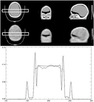
Figure 3. CT and scaled attenuation map from transmission from Lu-176 with 1 h acquisition (top) of a striatal brain phantom. Profiles (bottom) from the attenuation map created by the CT (-) and from Lu-176 transmission (◊) are compared.
Download figure:
Standard image High-resolution image2.2. MLACF reconstruction algorithm
After the initial estimation of the attenuation map from LSO background transmission imaging, attenuation is refined in simultaneous attenuation and activity reconstruction. In this work we used the MLACF algorithm presented in (Panin et al 2012) which extends the algorithm (Defrise et al 2014) for the case on non-zero background events. The scatter component is supposed to be known (since it cannot be updated without the attenuation map reconstruction) and the scaling parameter is defined by the initial estimate of the activity image. In the presence of a background the maximum likelihood estimate of the attenuation at fixed activity has no closed form expression. Therefore the algorithm approximates the attenuation by the maximizer of the non-TOF likelihood of the TOF summed data yi. This approximate ML estimate of the attenuation factor is equal to the ratio between the background corrected measured data, and the current modeled projection data (equal to the forward projection of the current activity image). Inserting this ratio into the original TOF Poisson likelihood eliminates the attenuation unknown so that the cost function becomes a function of the activity only. Optimization of that function is done using a monotone iterative algorithm with complexity similar to the commonly-used MLEM.
The attenuation of lines-of-response, passing outside the support of the activity image cannot be recovered in MLACF. For such LORs, MLACF uses known attenuation from transmission scan.
TOF prompt data y (511 keV window) with spatial projection (LOR) index i and TOF bin index t can be modeled by combining the modeled projection  from the emission object f, corrected for scanner efficiency by a normalization array N and for attenuation a. The background events have a known mean
  , equal to the sum of the estimated efficiency corrected scatter and of the estimated randoms. The Poisson Likelihood objective function has the following form:
where cit,j is the TOF system matrix. In the following, quantities without index t denote TOF summed quantities, e.g.

The attenuation factors that maximize the non-TOF likelihood of the TOF summed data yi at given activity are given by:
Here prime spatial projection indices denote LORs that have known attenuation. Substituting (6) into (4) leads to an objective function (the reduced log- likelihood as similarly defined in Defrise et al 2014) that can be maximized by the following iterative algorithm:
Here n is iteration number. We initialize the MLACF iteration (7) with the activity image reconstructed with one OSEM iteration using an initial estimate of the attenuation from LSO background transmission
3. Results
3.1. Rebinning of emission and transmission data
A phantom study was performed to demonstrate the ability to separate the emission and transmission data. A uniform phantom (20 cm diameter × 26 cm in height) with ~1 mCi of activity was placed on the bed next to a cold CT calibration phantom. Figure 4 shows the sinograms acquired simultaneously. The emission sinogram (bottom left) shows a 10 min acquisition and clearly shows the emission events with the shadowing of the cold CT phantom. The transmission sinogram (right figures) shows the collected data also for 10 min and separated by the gamma energies. In both transmission sinograms, both phantoms in the field of view are visible as well as the bed that the phantoms are placed on. All sinograms in the figures are displayed with the same polarity of greyscale.
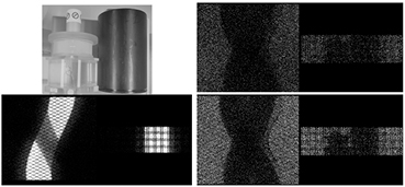
Figure 4. Photograph of the experimental setup with hot uniform phantom and cold CT calibration phantom with the corresponding emission sinogram (bottom left) and transmission sinograms of 202 keV gammas (top right) and 307 keV gammas (bottom right).
Download figure:
Standard image High-resolution image3.2. Contamination of transmission data from emission signal
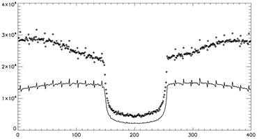
From figure 4, one can observe a noisier 202 keV sinogram when compared to the 307 keV sinogram. A study was performed to see if the transmission data was contaminated by the emission data and if the contamination is a function of emission source activity. 3 uniform phantoms (20 cm diameter × 26 cm in height) with varying activity from no activity to 0.5 mCi and 2.2 mCi were placed in the geometric center of the PET field of view. These phantoms were measured for 1 h and rebinned into the 2 transmission trues sinograms (prompts – delays). A profile across all the sinogram elements with summing over 100 angles and summing of all axial planes are shown in figure 5 for 202 and 307 keV transmission sinograms.
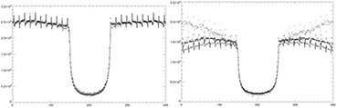
Figure 5. Profiles of the 307 keV (left) and the 202 keV sinograms. Profile is across all elements and sum of 100 angles and sum of all axial planes. No activity (-), 0.5 mCi (*) and 2.2 mCi (◊).
Download figure:
Standard image High-resolution imageThere is some contamination in the 307 keV transmission data around the edge of the object which can be seen as a small mismatch between the profiles. The 202 keV transmission data has more visible contamination from emission data. The tails of the sinogram increases in events further away from the center of the field of view. This may be a result of when the backscattering angle approaches 90° and the energies are close to equal to each other and both events fall into the 202 keV window. The change of the profiles in the region outside the objects boundaries in the cold phantom when compared to the region outside the object in the 307 keV profiles could be a result of the 307 keV photons scattering in the object into the 202 keV energy window.
3.3. Reconstructions of cold human volunteers
A study of human subjects was performed in order to observe how well the method performs for the complex structure of the human body. The scan duration times were set to 10 min to simulate fairly realistic scan times and minimize movement from the volunteers. Each volunteer was placed on the bed and inserted into the PET field of view with no activity in or around the PET scanner. A corresponding blank was acquired for 36 h and used for reconstructions of the attenuation maps. The reconstruction algorithm parameters used were 10 iterations with 24 subsets with some regularization for all human volunteer studies. No corrections were performed to the data that corrects for object originating physical effects to the transmission gamma such as scatter or attenuation.
Figure 6 shows two volunteer scans of the head with a carbon fiber head holder in the field of view. From the figure the sinus are visible and the head holder and outline of the head are well defined. Some high density regions are also visible such as parts of the skull and teeth.
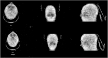
Figure 6. Reconstructed transmission image of volunteer's head with head holder. Acquisition performed for 10 min.
Download figure:
Standard image High-resolution imageFigure 7 are reconstructed images of the torso regions of males with weights of ~70 kg. The study of the torso region was performed with both arms up and arms down in a relaxed position. Arms are usually up in a clinical scan unless it is not practical. The arms down case can suffer from truncation of the CT. Using transmission data from Lu-176, the field of view for the attenuation maps are matched to the PET field of view. From both studies, body outline is resolved and internal details such as lungs and the heart are visible. The two studies also differ as the arms down case had the volunteer laying directly on the carbon fiber bed and the arms up case had the volunteer laying on a foam mat between the body and the bed. The bed is easily seen in both images but only having the whole bed visible when the volunteer is lying on a foam mat that separates the body from the bed. The patient's arms up while lying on the foam mat is the typical clinical procedure for imaging in the torso region.
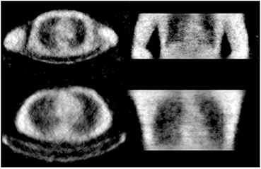
Figure 7. Reconstructed transmission images of volunteer's torsos. Studies were performed with both cases of arms down (top) and arms up (bottom) with acquisition time of 10 min.
Download figure:
Standard image High-resolution imageFigure 8 shows a larger volunteer of weight of ~ 180 kg that would experience truncation within the CT FOV. This study was performed with arms down and 10 min. The circle illustrates the CT's 50 cm FOV and demonstrates even if this study was performed with arms extended overhead, truncation would still occur to this volunteer. It is observed that the body contour is still resolved and some internal structures are visible such as the lungs and heart, but not as clear as the smaller volunteers' case.
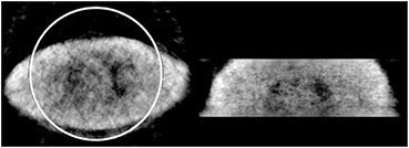
Figure 8. Reconstructed transmission image of large human volunteer. Circle illustrates the CT's FOV.
Download figure:
Standard image High-resolution image3.4. Reconstruction of emission data with Lu-176 attenuation maps
Work was performed to show the PET reconstructed images if the attenuation maps from the simultaneous transmission scan were used for the corrections to the PET emission data. The first case was a striatal head phantom with a fillable water cavity for addition of activity to the phantom. The phantom was filled with 4 mCi of F-18 and placed in a carbon fiber head holder. The phantom was scanned using a standard head-neck protocol for duration of 10 min. A corresponding CT was performed before the PET scan was acquired. The PET scan was the same for all three cases where the emission data was rebinned for 10 min into time of flight sinograms. Transmission based attenuation maps were reconstructed with a blank scan with duration of 36 h and the same reconstruction protocol used in the cold human studies above. Figure 9 shows three cases of interest, CT corrected, 1 h Lu-176 transmission and 10 min of Lu-176 transmission data. The 1 h collect of Lu-176 data was performed to show the quality of the method with higher statistics and compare it to a more reasonable time for patient studies. The attenuation correction and scatter corrections were performed using the associated attenuation map and the PET emission reconstruction performed was OP-OSEM with time of flight using 2 iterations and 24 subsets.

Figure 9. Attenuation maps derived from CT (top left), 1 h of Lu-176 transmission data (middle left) and 10 min of Lu-176 transmission data (bottom left). Images on the right show the PET emission reconstruction of 10 min of emission data from 4 mCi of F-18 (image positions correspond with attenuation maps used during corrections and reconstruction).
Download figure:
Standard image High-resolution imageThe PET emission data shows little difference between all three cases. Uniformity in all three cases also shows little differences demonstrating that the attenuation maps of this simulated brain scan are good enough to perform the corrections to the emission data even with 10 min of data.
An image quality phantom was scanned to extend the study to a torso sized object. The phantom was filled with Ge-68 in an epoxy matrix and had an activity approximately 2 mCi at the time of the measurement. The phantom has 6 spheres with 4 hot (4x activity concentration from background) and 2 cold spheres with a cold Styrofoam filled cylinder in the center of the phantom. The phantom was placed in the centered to the bore and set on top of the bed in a foam holder for this particular phantom. A CT was performed before the phantom was moved into the PET field of view. The listmode acquisition was performed for 30 min. The emission data was rebinned for 10 min acquisition time and all 30 min of transmission data for the 307 keV photons were rebinned for transmission data. The longer transmission scan was performed to account for the exclusion of 202 keV transmission data due to observed contamination of the 202 keV transmission data from the emission data.
Figure 10 shows the derived attenuation maps from the CT scan and from 30 min of transmission data from Lu-176. From the attenuation maps, it is observed that the cold cylinder in the Lu-176 transmission image is not well resolved. The corresponding PET emission images show some artifacts that come from having residual values in the cylinder that should be empty. This problem is not seen in the cold spheres because the spheres are filled with epoxy. The cross talk between the emission data and the attenuation map puts activity in the region where there should be air and no activity.
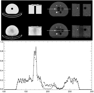
Figure 10. Attenuation maps derived from CT (top left) and from Lu-176 (bottom left). Images on the right are PET emission data reconstructed with 10 min of emission data from ~2 mCi of Ge-68. Lower plot is of the profile across the images shown by the white line in the above images using attenuation maps from CT (-) and Lu-176 (◊).
Download figure:
Standard image High-resolution image3.5. Reconstruction of emission data with Lu-176 transmission data and MLACF
The attenuation map created using the Lu-176 decays have some inaccuracies but are still useful for larger objects. These attenuation maps generally define the boundaries of the object being scanned fairly well. Using the Lu-176 attenuation maps, the scatter correction can be performed on the object and the resulting scatter correction sinogram is inputted to the MLACF algorithm. The Lu-176 attenuation map can also be used as a starting image for the attenuation estimate of MLACF. The image quality phantom's data from the previous section was reconstructed using the MLACF algorithm with 5 iterations and 24. The resulting emission and attenuation maps are shown in figure 11.
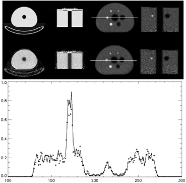
Figure 11. Attenuation maps derived for CT (top right) and estimated with MLACF (bottom right). Right images are the corresponding PET emission reconstructions. Lower plot is of the profile across the images shown by the white line in the above images using attenuation maps from CT (-) and Lu-176 with the MLACF algorithm (◊).
Download figure:
Standard image High-resolution imageThe attenuation map shown in figure 11 is an estimate from MLACF and shows that the internal structures are well defined with respect to the attenuation map derived from just Lu-176 data (figure 10). There is some disadvantage to the MLACF attenuation map in that there is no estimation for the line of responses that have no emission data. The bed and the shell of the phantom are not recovered but do not seem to vary much from the starting image. The center hole is recovered and the emission reconstruction now has no emission contamination in the center cold region of the phantom as seen in figure 10. Although the images are similar, the comparison is challenging as the two emission images are reconstructed using different algorithms with different objective functions and convergence rates. An observation is that the uniform regions do appear uniform with no visible artifacts. The sphere recovery is similar between the two cases and the iterations were selected to try to achieve similar noise structure between the two cases.
4. Discussion
The method of using the LSO background activity with time of flight information was demonstrated as a viable solution for attenuation correction of PET emission data. The method using direct attenuation maps scaled from Lu-176 transmission data is not likely to be used in the state demonstrated here for most typical scan protocols. It was shown that use of the technique as demonstrated may be feasible for brain studies. Since brain scan protocols are generally 10 min or more, the current technique could be implemented without much modification. The quality of the attenuation maps obtained from this technique is dependent on scan time and object size. As was demonstrated in the cold human studies, 10 min was enough time to obtain adequate attenuation maps, but was done so without the presence of emission radiation. If the contamination of the 202 keV energy window is corrected then 10 min should produce usable attenuation maps for patients. In this body of work, any addition of emission activity limited the data that could be used. Future work is planned to improve the current technique toward a more robust and consistent method. As demonstrated in this body of work, there are issues such as the contamination of the 202 keV transmission energy windowed data. This contamination occurred even with the condition to discriminate against backscattering events by using energy windows (section 2.1). Within this work, the issue was avoided by not using the 202 keV transmission data, but practically it is usable data if the contamination from backscattering 511 keV photons and 307 keV scattered photons are properly accounted for.
A thought to make the 202 keV data usable is to model the 511 keV backscatter events and correct for these events in the collected data or add information to the 202 keV blank collection sinogram. This would recover the events that are discarded when emission activity is present in the scanner's field of view. It also creates a new transmission type flux that adds to the Lu-176 flux that's presented here. The model would require some information on the emission flux and the emission volume's attenuation information. Both of these pieces of information are available from the current technique using only the 307 keV transmission data. Since it was shown that the 307 keV transmission data is mostly uncontaminated by emission data, the attenuation maps produced from this data can be used for the initial emission reconstruction. Using the emission distribution, a model of the backscattering of 511 keV photons can be performed to correct for the increase of counts not accounted for in the blank scan. This would allow for the removal of the condition where if the first event is in the 202 keV energy window, the second event cannot be in the 307 keV window. Figure 12 illustrates the additional information that can be acquired by not applying the backscatter condition to the 202 keV transmission data. The figure is a re-plot of figure 5 with 2.2 uCi and a cold 20 cm uniform phantom in the center of the field of view. It is seen that the addition of the backscattered events almost doubles the amount of events in the 202 keV transmission data. This increase of information is dependent on the amount of activity that illuminates the detectors.
Figure 12. Profile of 202 keV sinograms plotted the same as figure 5. The sinograms of the cold phantom (–) and the 2.2 mCi phantom (◊) were acquired and rebinned without the discrimination of backscattered events.
Download figure:
Standard image High-resolution image
Visible artifacts within the reconstructed transmission images can be observed that disturbs well defined boundaries especially in locations surrounded by some attenuating material such as the lungs or the empty region between the body and arms. This is attributed to object scatter of a transmission photon that still retains enough energy to be energy qualified. Using the attenuation maps as derived from the reconstructed transmission data results in emission reconstruction artifacts from attenuation-emission crosstalk as well as small errors in scatter correction using these attenuation maps. For the cases of the cold human volunteers, these scattered events may be more visible as the reconstruction used both transmission data sets. When using both energies of transmission data, the initial 307 keV photon can scatter into the 202 keV window resulting in a higher angle accepted scatter event. This would result in more scatter error if compared to using just the 307 keV windowed transmission data.
To correct for the scattered photons, a modeling of the 307 keV transmission data can be performed (Watson 2000, Vandervoort and Sossi 2008) with modification to the initial energy of the photon. The model of the 307 keV photons can also be performed with the scattering angles that fall within the 202 keV energy range. The 202 keV transmission data would also be scattered corrected and the result could be combined with the result of the scatter model of the 307 keV photons into the 202 keV energy window to create a complete scatter correction.
With all the fore mentioned improvements in the technique, the combination of the Lu-176 transmission data and the MLACF algorithm should also improve. In the current state the combination performs fairly well with respect to CT corrected PET images (figure 11), but the demonstration was with 30 min of transmission data. The improvements should enable for shorter overall scan times to obtain enough transmission events to perform good scatter correction to the emission data as well as a more refined starting image for the MLACF which will increases the algorithms convergence rate and proper scaling parameters.
5. Conclusions
Work was performed to demonstrate the feasibility of a transmission source that is already in all Lutetium based scanner. The technology that makes this work is the capability to measure time of flight of events detected by the PET scanner. With time of flight and some firmware modifications, simultaneous transmission and emission data can be collected. For some cases the transmission data acquired from the Lu-176 activity is enough to perform PET emission reconstructions. This method also can provide an attenuation solution to time of flight Lutetium based scanners that do not have or require a coupled CT scanner, such as MR-PET machines or dedicated PET machines with specific uses such as a brain machine. This work can be improved with more work to better refine the 202 keV events where emission contamination occurs. There may also be a way to use the backscatter events from the emission 511 keV gammas that could boost the signal even higher. In this work there was no work performed to improve the transmission images by making corrections to the transmission data such as scatter correction.
It was shown that the transmission images acquired simultaneously could be used to assist the MLACF algorithms to produce PET emission images close to CT corrected PET emission images. The attenuation maps from Lu-176 events were also of enough quality to produce a scatter estimate that was necessary as an input for MLACF. Combining the two techniques yields a solution for PET imaging without the need of an external imaging modality to assist with the collection of attenuation information. With the addition of corrections to the transmission data, the image quality of the PET images should approach the image quality of current PET/CT images.