
Abstract
An optimal experiment design methodology was developed to select the framing schedule to be used in dynamic positron emission tomography (PET) for estimation of myocardial blood flow using 82Rb. A compartment model and an arterial input function based on measured data were used to calculate a D-optimality criterion for a wide range of candidate framing schedules. To validate the optimality calculation, noisy time-activity curves were simulated, from which parameter values were estimated using an efficient and robust decomposition of the estimation problem. D-optimized schedules improved estimate precision compared to non-optimized schedules, including previously published schedules. To assess robustness, a range of physiologic conditions were simulated. Schedules that were optimal for one condition were nearly-optimal for others. The effect of infusion duration was investigated. Optimality was better for shorter than for longer tracer infusion durations, with the optimal schedule for the shortest infusion duration being nearly optimal for other durations. Together this suggests that a framing schedule optimized for one set of conditions will also work well for others and it is not necessary to use different schedules for different infusion durations or for rest and stress studies. The method for optimizing schedules is general and could be applied in other dynamic PET imaging studies.
Export citation and abstract BibTeX RIS
General scientific summary In the design of positron emission tomography (PET) experiments, parameters such as the amount of radioactivity, the speed of the radiotracer infusion and acquisition duration are chosen. In this work, we applied an optimal experiment design methodology to determine the sampling schedule of a time series of images that maximizes the precision of myocardial blood flow estimated using PET with 82Rb. This optimization is challenging because of the large parameter space, and we address the challenge using an exhaustive search of schedules which is made feasible and efficient by novel parameterization of the search space. We used Monte Carol simulation to validate the use of the D-optimality criterion for experiment design. Further, we made the experiment design robust by repeating the optimization over a range of infusion speeds, acquisition durations and physiologic conditions. The methods we developed could be applied to other applications of dynamic PET.
1. Introduction
Quantification of myocardial blood flow (MBF) using positron emission tomography (PET) has potential clinical application in detecting, monitoring, and evaluating the treatment of coronary artery disease (Ziadi and Beanlands 2010, Al-Mallah et al 2010, Camici and Rimoldi 2009, Kaufmann and Camici 2005). Compared to qualitative imaging, MBF may improve the detection accuracy of multivessel disease, improve the interpretation of subtle irregularities, and provide information regarding microvascular function (Yoshinaga et al 2003, Parkash et al 2004). MBF quantification uses a physiologic model to interpret dynamic cardiac PET data and produce flow estimates. A simplified, one-tissue-compartment physiologic model is favoured for MBF estimation as the data are typically noisy and the primary interest is in the transfer of radiotracer from blood to myocardial tissue over a time period of a few minutes (Klein et al 2010a, Choi et al 1999). The physiologic model equations are solved for presumed sets of parameter values, including an influx parameter K1 from which blood flow is calculated, to produce predicted time courses of myocardial radioactivity concentration. The flow value is determined as that of the model-predicted time course that best matches a measured time-activity curve (TAC) obtained from a dynamic sequence of PET images. To achieve the most precise and accurate blood flow estimates, optimizations of various aspects of the experiment design have been considered, including optimizing both the amount of activity and time course of radiotracer administration (deKemp et al 2006), reconstruction methods (Efseaff et al 2012), and the classification of image regions according to tissue type (El Fakhri et al 2005). In this work we consider the spacing in time of the frames in the dynamic PET series and, therefore, the spacing of samples in the TAC.
In optimal experiment design, data collection methods are designed in order to optimize some quantifiable measure. Herein, we maximize the precision (or, equivalently, minimize the variance) of the parameter estimates. Optimal experiment design has been used to refine PET experiments for estimation of physiologic parameters for application in receptor concentration (Delforge et al 1989, Muzic et al 1996) and glucose metabolism (Li et al 1996, Mazoyer et al 1986). Ho-Shon et al (1996) optimized the sampling schedule for whole-body FDG PET using multiple bed positions. Li et al (2000) studied the optimization of sampling schedules for cardiac FDG PET, using a glucose metabolism model with simultaneous estimation of the input function and tissue parameters. Their study concluded that a six-frame optimized sampling schedule performed as well as a conventional 19-frame schedule, confirming the value of an optimal experiment design approach to frame scheduling for PET-based parameter estimation. These successes of optimal experiment design motivated us to assess the value of optimizing the framing schedule for 82Rb-PET-based MBF estimation.
In this study, we optimized the time-framing schedule for MBF estimation, specifically using 82Rb-PET. Despite its known challenges, MBF with 82Rb is practical for clinical usage as 82Rb is generator-produced, has a short half-life, and a small radiation burden (Senthamizhchelvan et al 2010). Moreover, because 82Rb is retained in the myocardium, there is the potential that a qualitative perfusion image and MBF estimates can be obtained from a single infusion and acquisition. This capability is supported by on-going technologic improvements. The availability of list-mode data, which constitutes the emerging clinical standard, provides flexibility in time-binning. The availability of a PET scanner that couples high count-rate capability with time-of-flight information enables the high-activity bolus to be accurately captured as it flows through the heart while achieving effective sensitivity that allows the myocardial radioactivity concentration to be measured with reasonable precision multiple half-lives later. As such, the technology is ready to support the clinical use of 82Rb-PET to measure MBF, which is facilitated by using the optimized framing schedule that we describe herein.
A novel aspect of our work is the way we parameterize the space of possible framing schedules. Specifically, we consider framing schedules of the form, n contiguous frames of duration X, followed by m frames of duration Y, etc, which we denote as (n × X) + (m × Y) + ⋅⋅⋅ which allows us to efficiently do an exhaustive search of the space of possible framing schedules. Prior studies generally allowed the durations of all frames to be independently selected. While this greater flexibility has the possibility of yielding an even better protocol than ours, our approach is aligned with the way researchers conventionally define framing schedules and is, therefore, more practical to implement using software common on clinical scanners.
2. Methods
In determining the best acquisition duration and reconstruction frame schedule, our general approach is to use mathematical modelling and simulation to optimize and then validate the experiment design. The performance of different framing schedules is compared using calculated optimality criteria and simulation over a range of data representing different physiologic parameters, as well as infusion and acquisition duration. To ensure clinical applicability, the input functions, curve shapes, parameter values and noise model used in analysis and simulation are based on published and measured data. We combine all of these elements to establish a clinically relevant method for experiment design that is robustly optimal over a range of conditions. Details for each of these steps follow.
Human subjects data are used as the basis for modelling realistic input functions. Approval for this study was obtained from our institutional review board, and written informed consent was obtained.
2.1. Simulation of input function
We specify the input function in terms of a gamma variate function, which is capable of accurately reproducing TACs in the cavity of the left ventricle (LV) following a bolus injection. For convenience in estimating the input function model parameters, we describe the gamma variate Γ(t) in terms of parameters (Cmax, tmax) corresponding to the peak's amplitude and time, α for shape and t0 for time delay (Madsen 1992).

and where Γ(t) = 0 for t ⩽ t0. Whereas Γ(t) models in part the arterial activity concentration time course following a perfect bolus injection, we are interested in describing the arterial activity following 82Rb administered using an 82Sr/82Rb generator infusion system (Bracco Diagnostics Inc., Princeton, NJ), which typically delivers rubidium chloride over 5 to 25 s. To account for this, we convolve Γ(t) with a rectangular infusion pulse with unit area and duration tInf. We also add a rising asymptotic term, which represents a combination of equilibrium activity in the blood and spillover from the myocardial uptake due to partial volume and limited spatial resolution (Golish et al 2001), in order to obtain input function Ca(t) representing the time course of radioactivity concentration in arterial blood

where rect(t/tInf) equals 1/tInf on the interval t ∈ [0, tinf] and 0 otherwise, C0 is the steady-state value of the measured blood activity, and Ca(t) = 0 for t ⩽ t0. In clinical practice, we estimate Ca(t) from a TAC for a volume drawn in the LV cavity. The model-predicted PET measurement for arterial radioactivity concentration in the jth frame MCa, j is determined as the value of Ca(t) averaged over the duration of frame j, which spans the time interval from tj to tj+1.

To achieve clinically realistic input functions, we determined the values of parameters Cmax, tmax, C0, α, β, t0 and tinf by fitting (3) to the data obtained from five human, resting 82Rb scans. In these scans, PET data were acquired in list-mode on a Gemini TF-16 PET/CT (Philips Healthcare, Cleveland, OH, USA) (Surti et al 2007). The acquisitions began concurrently with infusion of 307 ± 60 MBq of 82Rb in 6 ± 2 mL of saline. At the peak count rate of each scan, we estimate that no more than 30% of the events were lost to system dead time and that with dead time correction the bias in the values was less than 5% of the true value.
Starting at the time at which activity arrived in the field of view, as judged by the singles rate exceeding 5% of background, PET data were binned into a dynamic time series with 20 frames each of 1 s duration (abbreviated 20 × 1 s), followed by 8 × 5 s, 17 × 15 s, and 2 × 30 s. The frames were individually reconstructed using a blob-based, list-mode OSEM algorithm (Popescu et al 2004) with correction for attenuation, scatter, randoms, dead time and radioactive decay. TACs for the LV cavity were generated from the data by taking the mean activity concentration over a 0.22 mL volume of interest drawn at the base of the heart in a short-axis view. To fit the TACs using (3), first values for Cmax, tmax and C0 were calculated from a fit to the peak and tail of the measured data, and then α, β, t0 and tinf were iteratively estimated using lsqcurvefit in MATLAB (Optimization Toolbox 6.2.1; The Mathworks, Inc., Natick, MA, USA). The means of estimated parameter values were used to construct the input function shape for subsequent simulation of tissue TACs; the variety of LV cavity TAC shapes among clinical patients was therefore not simulated.
2.2. Simulation of PET time-activity curves
To create simulated data for MBF estimation, we used the one-tissue-compartment physiologic model described by Hutchins et al (1990), who used ammonia as the radiotracer, and later applied to 82Rb by Coxson et al (1995). With noisy data, this model is a good choice as it facilitates a more reliable fit than multiple-compartment models (Coxson et al 1997). The model equation representing the activity concentration contributing to the myocardial PET signal is

where Ca(t) is the activity concentration in the blood and the convolution term represents the accumulated radioactivity concentration in the myocardium. The measured tissue activity was modelled as a function of parameters for uptake K1, washout k2, and a third parameter fv that accounts for both the vascular fraction and spillover from the LV cavity to the myocardium tissue region. The model-predicted activity in the jth contiguous image frame is calculated as the activity concentration time-averaged over the frame interval,

The integrals in (3)–(5) were numerically evaluated using CVODES (Serban and Hindmarsh 2005) as implemented in COMKAT (Muzic and Cornelius 2001, Fang et al 2010). Noise Σj was then added to the noise-free, model-predicted tissue concentration Mj to generate a simulated data value Dj. The noise in each frame was calculated by sampling from the standard normal distribution and scaling to achieve the specified standard deviation (SD; σ).

In our noise model, variance  was proportional to the number of counts contributing to that frame, which is calculated from the frame duration and a decay term (tH = 1.273 min) as the PET data were decay-corrected during image reconstruction.

The value of proportionality constant ξ was determined such that the average SD matches a value specified (e.g. 10% of Mj) for each set of simulated TAC.
To determine what noise level appropriately models that of clinical imaging, we scanned a torso phantom filled with 7.2 kBq mL−1 of 18F containing a cardiac insert filled with 100 kBq mL−1 (Data Spectrum, Hillsborough, NC, USA). Statistical replicate images, each with approximately the same number of counts as one frame of a human study, were created by splitting list-mode data into 1 ms intervals and dealing successive intervals into 20 data files to create 20 independent datasets with, on average, the desired number of counts. Each replicate data file was reconstructed, a volume of interest was drawn in the myocardium insert, and the SD among the replicate images of the volume's mean was calculated. Simulations were then focused on these clinically relevant noise levels.
2.3. Parameter estimation from simulated TAC
Values for the three parameters, K1, k2, and fv, of the physiologic model were estimated by minimizing a weighted least-squares (WLS) objective function:

where Mj and Dj are the values of the model output and measured (or simulated) data at frame j of the number nf of total frames and wj are weights, specified as reciprocals of the variance (Muzic and Christian 2006) and estimated from the number of counts in the frame, i.e. ξ2/σ2 in (7). For experiments in which parameter estimation is performed infrequently and the quality of the estimate can be verified by careful inspection, the WLS objective function can be minimized using nonlinear optimization. A more automated, efficient and robust method is desired for routine clinical use. Accordingly, we implemented a means to minimize the WLS objective function that takes advantage of certain properties of the model formulation. In particular, in the PET model equation, i.e. combining (4) and (5),

K1 can be factored outside the integral and it becomes evident that the equation is nonlinear in only the k2 parameter. In considering the values of functions time-averaged over each frame, we can write this as a vector-matrix operation,
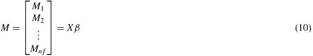
with
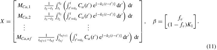
Given a specified arterial input function and value of k2, β was determined from the measured data by solving, in a least-squares sense,

where W is a diagonal matrix holding the weights wj for each frame. Indeed, the value of β that minimizes OWLS is available in closed form as

Therefore, for a given value of k2, fv = β1 and K1 = β2/(1 − β1) could be determined. This calculation was repeated for a list, i.e. a one-dimensional grid, of k2 values for each of which the value of OWLS was calculated. The value of k2 that gave the lowest value of the WLS objective function, as well as its corresponding K1 and fv, were taken as the optimal estimate of the parameter vector. This method of estimating the parameter values is similar to the linearized least squares approach (Koeppe et al 1985), which was extended to include a spillover term in studying blood flow in tumours (Lodge et al 2000). To simulate the use of an image-derived input function, we modelled the PET measurement of the input function for each framing schedule using (3), and then applied linear interpolation of the frame values as the 'measured' input function for parameter estimation.
2.4. Optimal experiment design
The goal of optimal experiment design is to maximize the sensitivity of the data to the parameters of interest in order to maximize the precision of the parameter estimates. Various metrics have been applied to quantify this sensitivity. We used a common one called the D-optimal criterion which entails maximizing the determinant of the Hessian (H), the matrix of second derivatives of the objective function with respect to the parameter values (Muzic et al 1996). The Hessian provides a measure of the steepness with which the objective function increases as one moves away from its minimum value with greater steepness yielding better precision of the parameter estimates. Maximizing the determinant of the Hessian corresponds to minimizing the volume of the confidence region. As the Hessian depends on the values of the parameters, to evaluate it we assumed representative values for the physiologic parameters, i.e. [K1, k2 and fv] = [1.0 mL g−1 min−1, 0.3 min−1, 0.3 (unitless)], and adjusted the values of the experiment design parameters, such as the infusion duration or framing schedule, as to maximize the determinant of the Hessian of the WLS objective function. We then tested such designs using Monte Carlo simulations wherein K1, k2 and fv values are estimated for a large set of simulated TACs.
The Hessian of the WLS objective function can be approximated in terms of the model sensitivity functions and weighting matrix W (Bard 1974).


where θ = [K1, k2, fv]' is the parameter vector. We maximized det(H) using two approaches. In the first, the schedule was parameterized as a list of independent frame durations with no gaps or overlaps between frames, and the optimal schedule was determined by minimizing  using an active-set algorithm available in MATLAB (fmincon, Optimization Toolbox 6.2.1; The Mathworks, Inc., Natick, MA, USA). We observed that when the sensitivity functions change only slightly between frames, the optimization methods had difficulty. As the results were sensitive to initial guesses and converged to local minima, we tried a second approach, an exhaustive search in which the frame durations were parameterized in clusters and also constrained to integer numbers of seconds. Three different frame durations were allowed in a framing design we denote as (n × X) + (m × Y) + (p × Z) + (1 × R), where n, m and p are the numbers of frames of respective durations X, Y, and Z seconds. A final frame of the remaining duration R was included to achieve a fixed, 6 min acquisition length. Naturally, n, m and p must be integers, and we restricted them to be values from 0 to 20, based on a cursory analysis showing diminishing returns with more than 60 total frames. While frame durations could be real numbers, in practice we considered integer values from 0 to 30 and also constrained Z ⩾ Y ⩾ X. Given the discrete problem, we calculated det(H) for each possible schedule in the search space. To gauge the potential of our approach for improving current practice, we evaluated published experimental protocols for MBF estimation (Lortie et al 2007, El Fakhri et al 2009, Raylman et al 1993, Sherif et al 2011). In the published schedules, we extended the final frame or removed frames as needed in order to match a fixed 6 min total acquisition duration. We then calculated det(H) for the published sampling schedules and for a schedule with the same number of frames, that had we optimized.
2.5. Robust experiment design
In the previous section, the framing schedule was optimized for a particular input function and assumed values of blood flow and other model parameters. In contrast, a clinical population represents a range of parameter values and an experiment design that works well in patients with normal physiologic function might work poorly in pathologic conditions. We addressed this by expanding the approach described in the previous section by considering four sets of physiologic parameter values denoted by A, B, C and D in table 1. Simulated subjects A and B were based on fits to stress and rest data obtained from healthy volunteers (Lortie et al 2007). Simulated subject C was based on fits to a canine model of ischemia under pharmacologic stress (Herrero et al 1992), and subject D was based on fits to the rest data described in section 2.1. The different spillover fractions likely reflect the variation in heart size, scanner resolution, motion, and image reconstruction methods. A 10% noise SD was used, as calculated from the phantom study described in section 2.2.
Table 1. Parameter values considered in calculating the robust design.
| Simulated subject | K1 (mL g−1 min−1) | k2 (min−1) | fv |
|---|---|---|---|
| A | 1.08 | 0.21 | 0.5 |
| B | 0.47 | 0.12 | 0.5 |
| C | 2.07 | 0.51 | 0.3 |
| D | 0.80 | 0.25 | 0.2 |
Using a minimax optimization, robustness is achieved by determining the schedule where the minimum objective function value is maximized—that is, minimax optimization identifies the schedule with the best worst-case performance, in our case according to the D-optimal criterion (Salinas et al 2007). As in the previous section, we calculated det(H) using an exhaustive search: for each framing schedule in the search space, we computed the determinant of the Hessian for each simulated subject. For each schedule, we identified the minimum value of det(H) using that schedule among the subjects; the schedule with the highest minimum det(H), or equivalently the lowest, maximum value of the objective function, was the most robust.
2.6. Infusion and acquisition durations
For 82Rb-PET, a slow infusion has been proposed as an alternative to a bolus-like infusion, in order to minimize both the scanner's dead time (deKemp et al 2008) and the temporal sampling requirements needed to capture the rapid dynamics (Raylman et al 1993). We modelled the duration of the tracer infusion by changing tInf in (2), covering a range of durations suggested in the literature, from a bolus (El Fakhri et al 2009) to a 4 min infusion (deKemp et al 2006) while holding the total injected activity constant. The D-optimality criterion was calculated for each duration, and Monte Carlo simulations were performed for selected durations to measure the precision of the parameter estimates. In this way we quantitatively evaluated the anticipated benefit of a rapid infusion. Infusion duration was studied at a fixed, 6 min acquisition.
We also studied the effect of modifying the duration of PET data acquisition in order to select a study duration that achieves high precision without excessively extending the scan duration into a region of diminishing returns. Using a fixed, 10 s infusion, the D-optimality criterion was calculated for data durations ranging from 0.5 to 20 min, using an optimized framing schedule for each duration. Selected durations were examined using Monte Carlo simulation, and the bias and precision of parameter estimates were calculated.
3. Results
3.1. Input function parameterization
The input function model was applied to TACs from the LV cavity seen in five human scans in order to obtain a typical curve shape. Table S1 (available from stacks.iop.org/PMB/58/5783/mmedia) shows the range of parameters describing the curves derived from the five images; figure S1 (available from stacks.iop.org/PMB/58/5783/mmedia) shows the model fit for the first subject. The normalized root-mean-square of the residual differences between the fits and data for the five subjects ranged from 6%–14%, suggesting that the input function model approximates the data well. The infusion durations estimated from the input function, i.e. 0.11–0.38 min, fell in the range typically reported by the infusion system. Based on the quality of these fits, we concluded that the mean curve, labelled 'Model' in table S1 (available from stacks.iop.org/PMB/58/5783/mmedia), was a plausible representation of a human measurement, and we used it as the input function for subsequent simulations. For simulating arterial input functions, we fixed the delay parameter at 3 s and the infusion length at zero to initially study a bolus-like infusion.
3.2. D-optimal criterion and simulations
The model sensitivity functions Ji, j and the D-optimal criterion  were first calculated for nominal values for the physiological parameter values, [K1, k2 and fv] = [1.0 mL g−1 min−1, 0.3 min−1, 0.3 (unitless)]. As expected, the sensitivity functions had the greatest amplitudes at early times and had distinct shapes, thus suggesting linear independence hence good local identifiability. The sensitivities are shown together and scaled to facilitate visual comparison of their shapes in figure 1(a). The D-optimal criterion was calculated from the sensitivity functions, for sampling schedules with uniform frame durations ranging from 0.5 to 15 s (720 to 24 equally-spaced frames), figure 1(b). As expected, more frequent sampling leads to an increased value of det(H) with very small improvements beyond approximately 180 frames, which corresponds to frame durations of 2 s.

Figure 1. Dynamic sensitivity functions (a) and D-optimal criterion (b) for the one-tissue-compartment model.
Download figure:
Standard image High-resolution imageNoise-free and noisy TACs were then simulated with uniformly spaced frames of 5 s duration. Noise was added according to (6) with a specified average SD ranging from 1% to 50%. Estimates for the physiologic model parameters were calculated as described in section 2.3 using a uniformly-spaced grid of 200 k2 values ranging from 0 to 1 min−1. Parameter estimation for 12 noise levels, each with 30,000 TACs, took 14 min on a standard desktop PC (running on four cores at 2.80 GHz). Using this number of TACs and 0.5% resolution in k2 was deemed to be more than sufficient to estimate the mean and SD of parameter estimates on the basis of cursory studies comparing 106 and progressively fewer TACs at high and low noise levels.
As shown in figure 2, the parameter estimates had low biases, i.e. bars are centred near zero error, and variances, i.e. the widths of the bars, decrease with noise level. The bias of K1, was less than 1% of the true value with noise levels up to 20% SD. The bias at the highest noise level (50% SD) was (3.4 ± 0.4)% of the true value (99% CI). This indicated that our noisy simulations and parameter estimates behaved as expected and that there was no evidence of programming errors.
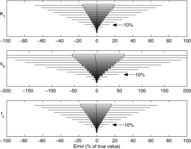
Figure 2. Distribution of errors in the estimated parameter value at 12 noise levels and simulated using uniform, 5 s frames. The noise levels are, from top to bottom, 50%, 45%, 40%, 35%, 40%, 25%, 20%, 15%, 10%, 5%, 2% and 1%. A noise level of 10%, noted with arrows, is typically observed in clinical data. Filled boxes: interquartile range (IQR); whiskers: ±1.5 · IQR; vertical hash: mean; outliers not shown.
Download figure:
Standard image High-resolution imageTo determine an appropriate noise level for subsequent simulations, we analysed the cardiac phantom data described in section 2.2. Volumes of interest were drawn in the cardiac insert portion of the phantom, corresponding to single image voxels (0.01 mL), and small, average and large segments (1.7, 3.5 and 5.0 mL) in a standard 17-segment cardiac model (Cerqueira 2002), as well as the entire LV myocardium (64 mL). As expected, image noise decreased smoothly with an increase in the number of coincidences or region size, figure S2 (available from stacks.iop.org/PMB/58/5783/mmedia). For subsequent simulations, we chose a noise level ξ = 0.1 which, when applied following (7), gave simulated TACs with a frame SD in the range of 4% (for a 15 s frame at 120 s) to 15% (for a 1 s early frame or a 15 s frame at 6 min).
3.3. Optimization of the framing schedule
In the first optimization method, the schedule was parameterized as a list of 13 contiguous frame durations. The quantity ![$\left[ {\det ( H )} \right]^{ - 1}$](https://content.cld.iop.org/journals/0031-9155/58/16/5783/revision1/pmb463817ieqn4.gif) was used as the objective function and was minimized using MATLAB's fmincon with an initial guess of uniform (18 s) frames (figure 3(a)) and constrained such that the sum of all frames equalled the 6 min study duration. As expected, the iterative optimization preferred numerous short-duration frames early after the arrival of activity and longer duration frames later, when the curve shape was not changing as rapidly (figure 3(b)). Iterative optimization was feasible with up to 13 frames with careful attention given to initial guesses, tolerances, and other optimization algorithm parameters in order to avoid local minima. Next, we exhaustively searched 13-frame designs following the parameterization method described in section 2.4. The optimal 13-frame schedule from the exhaustive search is shown in figure 3(c); its corresponding det(H) 8.71×10¹², slightly lower than the iteratively optimized 13-frame schedule (det(H) = 9.61×10¹²) shown in figure 3(b). The slightly higher value with iterative optimization is due to the iterative method having access to parameter values between those on the exhaustive method's grid. As expected, both optimization approaches yielded higher values for the objective function, and are therefore expected to provide better estimate precision, than the initial condition (figure 3(a)) with uniform frame durations (det(H) = 2.95×10¹²).
was used as the objective function and was minimized using MATLAB's fmincon with an initial guess of uniform (18 s) frames (figure 3(a)) and constrained such that the sum of all frames equalled the 6 min study duration. As expected, the iterative optimization preferred numerous short-duration frames early after the arrival of activity and longer duration frames later, when the curve shape was not changing as rapidly (figure 3(b)). Iterative optimization was feasible with up to 13 frames with careful attention given to initial guesses, tolerances, and other optimization algorithm parameters in order to avoid local minima. Next, we exhaustively searched 13-frame designs following the parameterization method described in section 2.4. The optimal 13-frame schedule from the exhaustive search is shown in figure 3(c); its corresponding det(H) 8.71×10¹², slightly lower than the iteratively optimized 13-frame schedule (det(H) = 9.61×10¹²) shown in figure 3(b). The slightly higher value with iterative optimization is due to the iterative method having access to parameter values between those on the exhaustive method's grid. As expected, both optimization approaches yielded higher values for the objective function, and are therefore expected to provide better estimate precision, than the initial condition (figure 3(a)) with uniform frame durations (det(H) = 2.95×10¹²).
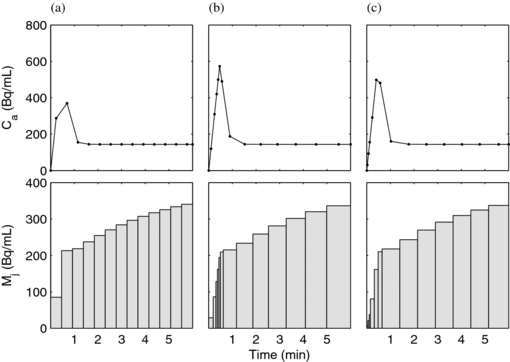
Figure 3. PET TACs with the same parameters shown with 13 frames following uniform spacing (a), optimized iteratively (b) and optimized in an exhaustive search (c). The top row shows the input functions, calculated as a linear interpolation of the PET-sampled LV cavity measurement as would be done with experimental data. The bottom row shows the noise-free PET TACs representing the myocardium region.
Download figure:
Standard image High-resolution imageThe experiment design in figure 3(c) is one of many considered in the exhaustive search process. Figure 4 shows the det(H) calculated for the range of the exhaustive search. Among each column of points, which represents a fixed number of frames, the top-most point has the highest det(H) and is the optimal design for that number of frames. We found that for any number of frames, the optimal schedule gave a higher det(H) than any optimal schedule with fewer frames. The more-optimal schedules tend to have several short frames clustered early, when the signal is changing rapidly and near the sensitivity functions' maxima, and longer frames at later times, following the overall pattern seen in figures 3(b) and (c). As examples, the optimal schedules for 5, 10, 20 and 50 total frames are noted in figure 4 by stars. Those schedules are
.
| 5 frames: | 1 × 5s | + | 1 × 20s | + | 2 × 60s | + | 1 × 215s |
| 10 frames: | 2 × 3s | + | 3 × 10s | + | 4 × 60s | + | 1 × 84s |
| 20 frames: | 4 × 2s | + | 6 × 5s | + | 9 × 30s | + | 1 × 52s |
| 50 frames: | 20 × 1s | + | 14 × 2s | + | 15 × 20s | + | 1 × 12s |
We then compared det(H) for our optimized schedules to experiment schedules described in literature. The schedules described in literature are described in table 2 and indicated in figure 4 by triangles. In all cases our design optimization was able to determine sampling schedules that improved the previously published schedules.
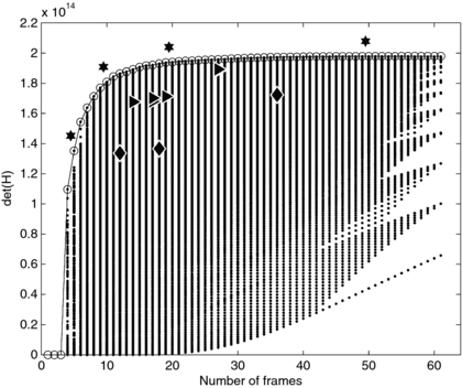
Figure 4. Values of the D-optimal criterion calculated using the exhaustive search method. The optimal schedule with each number of frames, at the top of each column of points, is circled. The schedules marked with stars are enumerated in the text. Diamonds mark examples of uniform sampling with 12, 18 and 36 frames. Triangles denote literature-derived scanning designs as detailed in table 2.
Download figure:
Standard image High-resolution imageTable 2. D-optimality calculated for various schedules described in literature and used for PET MBF estimation, with values for the optimal schedules with the same numbers of frames.
| Reference | Schedule | det(H) (1014) | Frames | Optimized det(H) (1014) |
|---|---|---|---|---|
| Lortie et al (2007) | 12×10 + 2×30 + 1×60 + 1×120 | 1.679 | 16 | 1.920 |
| Sherif et al (2011) | 12×10 + 6×30 + 1×60 | 1.713 | 19 | 1.937 |
| El Fakhri et al (2009) | 14×5 + 6×10 + 6×20 + 1×110 | 1.886 | 27 | 1.958 |
| Raylman et al (1993) | 10×10 + 3×20 + 3×60 + 1×20 | 1.702 | 17 | 1.920 |
| Raylman et al (1993) | 20×5 + 3×20 + 3×60 + 1×20 | 1.892 | 27 | 1.958 |
| Klein et al (2010b) | 9×10 + 3×30 + 1×60 + 1×240 | 1.677 | 14 | 1.892 |
To investigate the correspondence of det(H) and the precision of the flow estimate, MC simulation was performed for the a subset of the most promising schedules. Figure 5(a) shows that the optimal five-frame schedule performed poorly, thus resulting in a wide and non-normal distribution of parameter estimates, and that the optimal 10, 20 and 50 frame schedules performed progressively better, with estimates clustered closer to the true parameter values with a larger number of frames. We expanded the analysis using a larger number of schedules, selected the 44 schedules with the highest det(H) for each total number of frames from 17 to 60, and constructed a scatter plot of the precision of the K1 estimate versus det(H) (figure 5(b)). This demonstrated that the standard deviation of K1 estimates decreased with increasing det(H) and thus provided evidence that det(H) is a valid predictor of estimate precision and appropriate for use in experiment design.
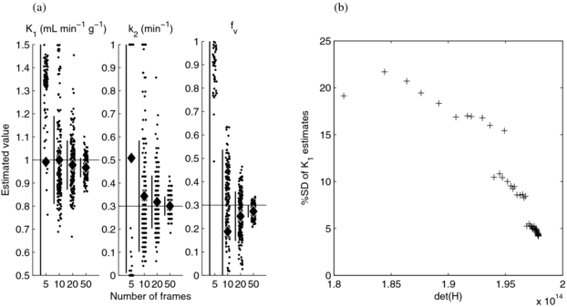
Figure 5. Simulation results for the D-optimal schedules. Parameter estimates using 5, 10, 20 and 50 frame schedules (a). Each column shows individual results as points (for visual clarity, a randomly selected subset is shown), the estimates' mean (diamond) and ±SD (vertical bar); the horizontal lines show the true parameter values. Standard deviation of the K1 estimates versus det(H) for 44 schedules (b).
Download figure:
Standard image High-resolution image3.4. Robust design
We calculated det(H) and performed Monte Carlo simulations for a range of schedules, infusion lengths and physiologic parameters, with the goal of determining a single schedule applicable to the patient population. We examined the 30-frame schedules in our exhaustive search parameterization, having observed that much of the available det(H) in the entire grid is reached with 30 frames (figure 4) and that 30-frame images are manageable in research and clinical use. Figure 6 shows schedules, ordered in descending values of det(H) for subject C since this had the poorest det(H) therefore is the controlling subject for the robust design. The first schedule thus is the minimax or optimum for the robust design and consists of 29 1 s frames followed by a single, 331 s frame (29×1 + 1×331). In comparing two schedules, generally one which performed poorer for subject C also performed poorer for the other subjects although there are exceptions to this as indicated by jumps in the det(H) curve such that it is not monotonically decreasing. However, focusing on the first 1000 schedules, figure 6(b), reveals that the rank-ordering of the best-performing schedules shows similarities across subjects. That is, many of the best schedules for subject C were also among the best for A, B, and D.
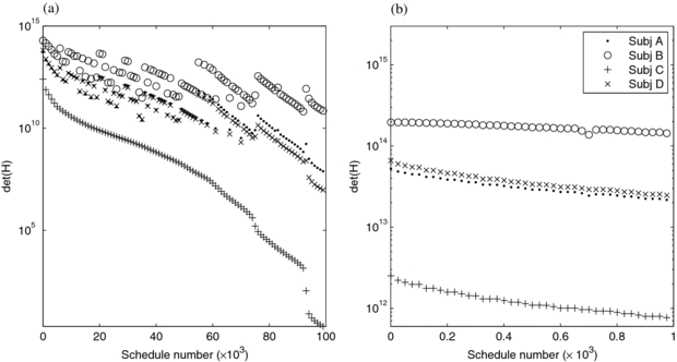
Figure 6. det(H) for the 30-frame schedules, for four simulated subjects are plotted versus schedule number. Schedules are numbered in terms of descending values of det(H) for subject C, so the curves for C descend monotonically while those for the other subjects have jumps. In (a) the top 100 000 schedules are shown. (b) shows a zoomed view of the top 1000. Every 1000th (a) and 25th (b) schedule is shown, for visual clarity.
Download figure:
Standard image High-resolution image3.5. Infusion and acquisition durations
Up to this point we considered an infusion of minimal duration (tinf = 0) because we expected short infusions to require the most demanding framing schedule and because requiring a different framing schedule for each infusion duration might not be practical for clinical use. We explored the validity of this approach by evaluating the effect of infusion length, determined by calculating det(H) for a range of values of tInf in (2). The D-optimal criterion was first calculated using fine, i.e. uniform 1 s, frame sampling to ensure that there was sufficient time resolution in order to capture the dynamics and decouple the problem of optimizing the infusion length from the problem of optimizing the framing schedule. As expected, the optimality was highest for the shortest infusion duration (figure 7), although infusions shorter than 3 s offered only slight additional benefit, i.e. an infusion of 3 s achieves 98% of the maximum det(H) of a 0.25 s infusion. This result suggests that a short, 3 s infusion is nearly as effective as a bolus injection. Next, the det(H) calculation was repeated with 1, 5, 15, 30 and 60 s infusion lengths, with a range of schedules in order to determine a robust schedule for use with different infusion durations. Subject A's physiologic parameters were used. For the 1 s infusion, a schedule with rapid initial sampling was optimal, i.e. (20×1 + 20×2 + 20×10 + 1×100). Schedules with slightly longer initial frames were optimal for slower infusions; for the 60 s infusion, the optimal schedule was (40×3 + 20×10 + 1×40). As with the physiologic parameter results, the rank order of schedules for each infusion duration was similar, and many similar schedules gave similar det(H) values for a given infusion duration. As shown in figure 7, the five schedules that are optimum for each of the five infusion durations are nearly optimal when applied to data simulated with each of the other infusion durations. Applying the optimal schedule for a 60 s duration to all infusion durations, in order to maximize the minimum det(H), still gives at worst 98.5% of the optimal det(H) and an increase in K1 SD from 3.5% to 3.6% of the its true value. Bias was examined using simulation and was not significantly affected by the infusion duration; this is consistent with our choice of 1 s time sampling for this part of the study.

Figure 7. D-optimality decreases with increases in infusion duration (a). The four most-optimal schedules in the search space perform well for all four infusion durations. Although their rank order differs as seen in the zoomed views (b), the det(H) values are quite similar.
Download figure:
Standard image High-resolution image
The preceding simulations were performed using a fixed, 6 min acquisition duration. We studied the effect of acquisition duration by simulating acquisition durations ranging from 30 s to 20 min, using 10% noise, uniform 1 s frame durations, and a clinically realistic, 10 s infusion duration,. Acquisitions of 4 and 6 min' duration achieved 95% and 99%, respectively, of the maximum det(H) of the longest (20 min) acquisition. The standard deviation of the estimated K1 and k2 values from simulated data followed a similar pattern, with little change between the 6 min and 20 min acquisitions. Bias was detected in K1 and k2, although it remained less than 1.5% of the true parameter values.
4. Discussion
Although optimizations of various aspects of experiment design have been considered for MBF determination, the framing schedule of the dynamic PET series used in parameter estimation had not been previously studied. Therefore, we sought to determine sampling schedules that would give the best data for precise estimation of blood flow as well as study their robustness over a range of anticipated physiologic parameter values as we are interested in clinical applicability.
We implemented a method of parameter estimation in which the model equation is factored such that some of the model parameters can be calculated analytically, while gridding over values for the remaining parameter. This method avoids two limitations of iterative estimation, i.e. the need to specify initial conditions and possible convergence to local minima. A potential disadvantage of our approach is that precision in k2 is dependent on the spacing of the pre-defined list of values, although this can be mitigated by setting the grid spacing to be finer than the estimate precision achievable in actual clinical practice. Decomposing a model in this way, for computational efficiency and robustness, has recently been discussed (Kolthammer and Muzic 2011, Oktay and Kadrmas 2012). For estimating the flow from a large number of data TAC that share a common input, we found that this parameter estimation method was computationally efficient. This was the case in this work in which ∼105 noisy TACs were analysed for each protocol as well as in our experience with human data when used to generate a parametric image with ∼103 voxels.
Optimization of the framing schedule in which frame durations varied independently, was challenging. Initially, we used an iterative algorithm to optimize the nonlinear det(H) objective function. We concluded that an exhaustive search, made feasible by describing the schedule in terms of a special parameterization, improved the reliability of the experiment design optimization. Although in practice list-mode PET data give us the flexibility to define finer frame intervals or to use unique durations for all frames, there is little to be gained by considering more complex framing schedules, as demonstrated by the similarity in det(H) among closely-related schedules, figures 3 and 4. We confirmed that the experiment designs used for PET-based MBF in the published literature perform better than uniform frame durations, although further improvement is available by choosing a schedule that maximizes the D-optimal criterion (triangles in figure 4). Of course, available framing rates, infusion speeds, count-rate performance, and other local factors play a role in selecting a schedule. Although our results indicate only an incremental benefit in the precision of flow estimation by extending the duration from four to 6 min, we primarily used a 6 min acquisition duration in order to also support generation of clinical, qualitative 82Rb myocardial perfusion images from the same injection (Dilsizian et al 2009). Our conclusions are therefore applicable to a protocol in which the same data acquisition is used for both modelling and also perfusion imaging. Indeed, Efseaff et al (2012) concluded that extending the study from 6 to 10 min was not helpful.
As expected, the optimal schedules have short initial frames and longer later frames, consistent with common practice and our analysis of the model sensitivities (figure 1). Furthermore, rapid early sampling aids in accurate derivation of the input function from the image-sampled blood activity, which was not considered by the D-Optimality calculation but was considered in our simulation. When comparing the results for 5 through 50-frame schedules, an increase in the number of frames resulted in improved precision following a pattern of diminishing returns (figure 4). Monte Carlo simulation showed expected distributions of parameter estimates, including discretized values for k2 aligned to the specified grid (figure 5(a)). Although det(H) increased smoothly across the optimal schedules for each total number of frames, the precision of the K1 estimate jumped downward in two regions (figure 5(b)). These regions were found to correspond to the locations where the optimal design switched from 3 to 2 s initial frames, and then from 2 to 1 s initial frames; they are thus an artefact of the schedule parameterization. Repeating the analysis for four simulated subjects, representing a range of rest and stress-like physiologic conditions, we found that with 30 frames the optimal schedule for the most challenging subject provided higher det(H) values for the other subjects, and thus making it the robust choice overall. This result suggested that there may be little to be gained from modifying the framing schedule based on anticipated parameter values or from using a different schedule for rest and stress scans.
Studying infusion duration is of particular interest because clinical studies typically specify activity and this necessitates lengthening the infusion as the 82Sr parent of 82Rb decays over the clinically useful lifespan of a 82Sr/82Rb generator. Despite this 82Sr decay issue, we found shorter infusion durations to be preferable, although some previous publications have proposed extending the infusion under some circumstances. In particular, Raylman et al (1993) recommended a 30 s infusion in order to avoid biased flow estimates caused by limitations in the framing rate. Efseaff et al (2012) also used a 30 s infusion so as to avoid excessive scanner dead time, and deKemp et al (2006) proposed using up to 4 min to allow an increase in administered activity. We found that 2 s initial frames were sufficient (in that no bias was detected) for use with a 5 s infusion of 82Rb from our generator system and yielded approximately a 10 s pulse width in the LV cavity. Therefore, we conclude that when framing rates and scanner dead time are not limiting, a short, tight bolus of very high activity concentration would offer the most precise flow estimates.
This study is predicated on a workflow in which images are reconstructed in a dynamic sequence, and then TACs are derived from the images. Reconstructing the physiologic parameter values directly from the PET data (Tsoumpas et al 2008) is a promising, alternative approach but is not yet commonly available in the clinic. We identified a framing schedule optimized for 82Rb-PET, but which may not be optimal for use with other perfusion tracers such as [13N]NH3 or newer, 18F-based agents (Berman et al 2013) which have different half-lives and noise characteristics. Nevertheless, the methods we developed could be applied in order to optimize the framing schedule for these tracers and even for other study types.
In this study, we focused on the estimation of all compartment model parameters, although it is MBF that is of particular clinical interest. An alternative approach suitable for future studies might be to apply a nuisance parameter factorization of the D-optimal criterion in order to focus solely on flow (Morris et al 1991). As MBF is typically modelled as a nonlinear but single-valued function of the K1 parameter (Lortie et al 2007), the ranking of schedules by MBF and K1 is equivalent, although imprecision in the flow estimate is magnified compared to that in K1 due to partial extraction, such as is the case with 82Rb at high flow. In this study we assumed the radioactivity measurements provided by PET imaging followed a particular noise model: variance is given as in (7) and the mean noise is zero. Future work could expand the analyses to explicitly account for noise and bias specific for a particular image reconstruction method. For example, iterative reconstruction methods may exhibit bias when there are low counts per frame. A Monte Carlo simulation approach could be employed to assess the impact of physical factors such as positron range and scanner dead time, could better account for real-world limitations. Although we simulated only four sets of physiologic parameter values, as there were many robust schedules, i.e. schedules that were optimal for one set of parameters were also highly ranked for the other sets, we anticipate that their robustness will be sufficient for clinical use. Furthermore, the differences in det(H) and the precision of the simulated parameter estimates were much less than other clinical sources of imprecision, such as same-subject repeatability (Manabe et al 2009, El Fakhri et al 2009, Efseaff et al 2012).
5. Conclusions
The influence of the framing schedule on myocardial blood flow estimation has been investigated for 82Rb-PET. We used an optimal experiment design approach, in which the D-optimal criterion was calculated for a wide range of possible schedules, after which simulation was used to validate the experiment design. Physiologic parameter values, input function shape and the simulation noise model were based on measured data. Efficient and robust parameter estimation for many simulated TACs was performed by factoring and analytically solving the estimation problem. The optimization methods offered improvements to previously used experiment schedules, and the results showed that optimal schedules were robust over a range of simulated physiologic conditions. The methods and structure of our study could be applied to other tracers and dynamic PET imaging studies.
Acknowledgments
We would like to thank James K O'Donnell, MD and Patrick Wojtylak, CNMT for their assistance in obtaining human data, Anu Grover, MS for phantom measurements, and Bonnie Hami, MA for editorial assistance in the preparation of this manuscript. This work was supported in part by an Ohio Third Frontier Medical Imaging Program grant (TECH 11-046) from the State of Ohio Department of Development.