

Abstract
Gravity racing can be studied using numerical solutions to the equations of motion derived from Newton's second law. This allows students to explore the physics of gravity racing and to understand how design and course selection influences vehicle speed. Using Euler's method, we have developed a spreadsheet application that can be used to predict the speed of a gravity powered vehicle. The application includes the effects of air and rolling resistance. Examples of the use of the application for designing a gravity racer are presented and discussed. Predicted speeds are compared to the results of an official world record attempt.
Export citation and abstract BibTeX RIS
Introduction
Gravity racers are one of the simplest designs of a vehicle relying only on gravitational force to derive forward motion. Known as soapboxes or downhill go-karts, the vehicle class of gravity racers are fitted with a four-wheeled chassis. Aside from recreational use, gravity racers are often raced competitively down defined runs, with time to complete being the performance criteria. The first All-American soapbox derby was held in 1924 [1] and design guidelines for competitors were provided in a series of articles published in Popular Mechanics [2]. Although the traditional format of gravity racing still exists today, there are a number of other events that allow for more advanced and creative designs of racers in competition; for example, Goodwood Festival of Speed, Red Bull Soapbox Challenge and the Xtreme Gravity Racing Series. With the absence of a motor, ease of construction and relatively low costs, gravity racing is a readily accessible sport to the public and ideal for school or youth organisation projects.
Although simple in concept, the design of a gravity racer requires an understanding of a number of physics and engineering topics. As well as providing students with a practical engineering challenge, a gravity racer project can also make an excellent physics case study for investigating Newton's second law. In this paper, it is shown how a Newtonian model, formulated and solved in Microsoft Excel™, can be used to predict the speed of a gravity racer.
Spreadsheet software such as Microsoft Excel™ are readily available, accessible to students at most schools, and popular for the demonstration and instruction of simple mathematical concepts and scripting in academia. They have been used extensively in the demonstration of projectile trajectories by solving Newton's equations of linear motion [3–5], and in the prediction of the speed of a track cyclist [6]. The application present here is a variant of these, and begins by resolving the forces acting on a gravity racer when rolling down an inclined slope. The purpose of the application is not only to provide students with a tool that aides understanding of how the design parameters effect the speed of the racer, but also to demonstrate how easily a student can script, modify and solve the equations using a spreadsheet. With experience, the application can be extended to include the effect of other parameters such as deceleration for cornering or influence of cross winds. Readers are referred to CartieSim (a race prediction tool developed by the Scottish Cartie Association [7]) for examples of how the application presented in this paper could be developed further.
Theory
A gravity racer travelling down an inclined slope will be subject to the forces shown in the free-body diagram, figure 1. Three main forces act in the direction of motion of the vehicle; (i) force due to gravity (FW), (ii) air resistance during motion (drag) (FD) and (iii) frictional force between the vehicle and the surface (FR). Using Newton's second law, we can determine the acceleration of the vehicle, a by resolving the forces acting upon it (equation (1)).

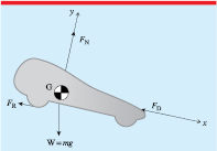
Figure 1. Free-body diagram.
Download figure:
Standard image High-resolution imageWhen moving down a slope of angle θ, the force due to gravity can be written as

where m is the mass of the vehicle.
The net aerodynamic force, FD acting against the moving vehicle is a property of the speed of the vehicle (v), the density of the air (ρ) and two design parameters: drag coefficient (CD) and the frontal area of the vehicle (A). The magnitude of the force can be calculated from
Considering a wheeled vehicle, the second resistive force is known as rolling resistance, FR. Rolling resistance is a measure of the force required to overcome the friction between the tyres and the road surface. This varies according to the normal contact force (FN) and is influenced by a number of different variables such as: tyre pressure, temperature, surface roughness and wheel diameter. Here, we have grouped the combined effect of these into a constant known as the coefficient of rolling resistance, μR and thereby simplifying our rolling resistance equation to

By substituting the resolved forces (equations (2)–(4)) into Newton's second law (equation (1)) we obtain
Rearranging equation (5) gives the equation of motion describing the acceleration of the vehicle, a
The solution to equation (6) allows the speed of the vehicle to be predicted at any given point on a potential course. This can be determined by considering that the velocity of the vehicle is the derivative of the displacement with respect to time, and the acceleration of the vehicle is the derivative of the velocity with respect to time (or second derivate of displacement). This expresses the equation as an ordinary differential equation (ODE), and for a given a time-step (Δt) the solution can be attained using the Euler method in which


where xn is the displacement at time t; and xn+1 is the displacement at time t + Δt; similarly for velocity and acceleration.
Spreadsheet application
The equation of motion can be solved iteratively using the Euler approach within a spreadsheet application such as Microsoft Excel™. Our application is shown in figure 2. Input variables are presented in cells A7:C16 and the solution shown as a line graph of displacement against velocity over 2000 m. The forces are calculated in range columns H to J using equations (2)–(4) and the resultant acceleration in column L using equation (6). Displacement and velocity are calculated in columns F and G respectively, using equations (7) and (8). The cell formulas are shown in table 1. Equations can be expanded down to as many cells as necessary to achieve the required distance. A time-step of 0.05 s was used for this simulation. The time-step influences the numerical error resulting from the Euler method. When a constant gradient slope is modelled, larger time-steps (such as 0.5 s) can be used without affecting the predicted speed. When changes of gradient are introduced, the model becomes more sensitive to the distance calculation and as such requires smaller a time-step to eliminate the propagation of error.
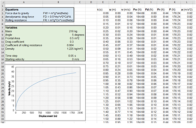
Figure 2. Screenshot of spreadsheet application (Microsoft Excel™).
Download figure:
Standard image High-resolution imageTable 1. Spreadsheet formulas used in the application.
| Measure | Cell | Formula |
|---|---|---|
| Time, t | E4 | =E3 + 0.05 |
| Distance, x | F4 | =F3 + G3 * 0.05 |
Speed,  |
G4 | =G3 + L3 * 0.05 |
| Force due to gravity, FW | H4 | =$B$8 * 9.81 * SIN($B$9*PI()/180) |
| Drag force, FD | I4 | =0.5 * $B$13 * G4^2 * $B$11 * $B$10 |
| Rolling resistance, FR | J4 | =$B$8 * 9.81 * $B$12 * COS($B$9 * PI()/180) |
| Total accelerating force, FA | K4 | =H4-I4-J4 |
Acceleration, a or  |
L4 | =K4/$B$8 |
The Microsoft Excel™ function VLOOKUP can be used to quickly obtain the speed of the racer at any given distance (equation (9)).

Utilisation in gravity racer design
Design analysis
The variables in the equation of motion (equation (6)), as listed in figure 2, are either: a factor of design, or a result of venue choice; all of these in theory can be controlled by the designers. However, scenarios often exist where it may not be possible to optimise all the variables in question. As such, it is important to be able to understand the influence choices in shape, mass and slope angle may have on the maximum speed of the vehicle.
A one-way sensitivity analysis was performed using the spreadsheet application to determine the percentage difference in velocity (figure 3). This was based on a theoretical run length of 2000 m when each independent variable was increased or decreased by 20% from an initial baseline. Baseline values were set using figures obtained from preliminary research of existing gravity vehicle designs; the 20% range limit was based upon realistically achievable improvements or compromises that could be made to racer design or venue.
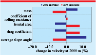
Figure 3. One-way sensitivity analysis of design parameters effecting final speed of the gravity vehicle (baseline values, m = 180 kg, μR = 0.004, A = 0.5 m2, CD = 0.3 and θ = 5°).
Download figure:
Standard image High-resolution imageThe analysis showed that venue selection was an important consideration for achieving the highest velocity, with a 1° increase in slope angle affecting the velocity by 14%. When competing in a gravity racer event, the course is defined and slope angle is not a factor that can be influenced by the competitors. However, if wanting to obtain the maximum possible speed a hill that has a large change in elevation over its distance (and hence large slope angle) would be advantageous.
When considering the design of the vehicle, the mass, drag coefficient and frontal area could increase or decrease the velocity from 5 to 8%. The drag coefficient and frontal area elicit the same percentage change in velocity due to their equivalent weighting in the drag force equation (equation (3)). It is possible for objects to have the same frontal area but differing drag coefficients due to variations in shape [8]. As such, it is important that both are considered in the design stage. Over this range, the rolling resistance had minimal effect, but it is worth noting that a simplified formula for rolling resistance was used in our application. Students may wish to investigate a more complex measure of rolling resistance based on experimental results [9].
Simulation of variable slope angles
The application presented solves for slopes of constant gradient (fixed slope angle, θ). In reality, it is uncommon for gravity race events to be held at venues with a constant gradient; it is necessary therefore to be able to include a variable slope angle in the above application. This can be achieved by the inclusion of an additional column (M) in which θ is defined. The force due to gravity, FW (column H, equation (10)) and rolling resistance, FR (column J) are then calculated using this value of θ rather than that originally defined in the input variables.

In many cases, θ may be determined by the distance along the course. In these instances, a series of IF statements can be used to define θ. For example, if slope angle changes as detailed in table 2:
Table 2. Variation in slope angle over a course distance of 2000 m.
| Distance | θ |
|---|---|
| 0–500 m | 5° |
| 500–1000 m | 10° |
| 1000–2000 m | 7° |
the formula in cell M4 can be written as:
Additional IF statements can be included in equation (11) to reflect the number of slope changes during the course.
Prediction of speed
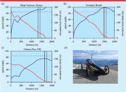
The presented spreadsheet application was developed as part of a project to design and build a gravity racer intended for use in setting an official World Record speed [10]. The final design parameters of our gravity racer (table 3) were used in the application to assess whether a record speed was achievable at a number of potential venues: Mont Ventoux in France, Teutonia in Brazil and Crimea Pass in Wales. Slope angle was updated using a variant of equation (11), determined from the elevation and distance profile of the courses obtained from free to use mapping software [11]. The elevation data was available approximately every 150 m along the course. Between data points, a constant gradient was assumed; in some instances, this can lead to uneven velocity profiles as shown in figure 4. Guinness World Records, the official record adjudicators, set a target value of 84.4 mph (a speed unofficially recorded by an American racer, Bodrodz Atomic Splinter in September 2012 [12]) which needed to be surpassed for the record to qualify. The frontal area and drag coefficient values were obtain from a computer aided design (CAD) model and computational fluid dynamics (CFD) simulation undertaken during the design stage of the project.
Table 3. Final design parameters of gravity racer developed for World Record challenge.
| Design parameter | Value | Design parameter | Value |
|---|---|---|---|
| Mass, m | 200 kg | Drag coefficient, CD | 0.26 |
| Slope angle, θ | Variable | Coefficient of rolling resistance, μR [13] | 0.004 |
| Frontal area, A | 0.42 m2 | ||
| Air density, ρ | 1.225 kg m−3 |
Figure 4. Predicted top speed of the racer design at three potential venues (a) Mont Ventoux (91.0 mph), (b) Teutonia (98.5 mph) and (c) Crimea Pass (76.4 mph), (d) final build of the racer at the summit of Mont Ventoux. Red line = elevation profile, black line = predicted speed, dashed horizontal line = target record speed, solid vertical lines = final speed measurement distance.
Download figure:
Standard image High-resolution image
The model predicted that it was possible to break the record at Mont Ventoux and Teutonia, but that insufficient speed would be achieved on the Crimea Pass course (figure 4). Although potentially not as fast as Teutonia, Mont Ventoux was chosen as the final destination based on safety concerns; Mont Ventoux has a superior road surface and a wider track allowing for the positioning of safety crash barriers. A further consideration was travel logistics; Mont Ventoux was both easier and more cost efficient to access from our location in the UK.
At Mont Ventoux, the model predicted that for a combined driver and vehicle mass of 200 kg our racer was capable of reaching a speed of 91.0 mph (40.7 ms−1) over the final 100 m of the course prior to the braking zone. The record-breaking attempt took place in October 2014 over a period of two days. After a number of test runs, and fine-tuning of the racer set-up, a new world record of 85.6 mph (38.3 ms−1) was achieved. The application had over predicted the top speed of the racer by 5.4 mph (6.3%). Considering assumptions made, and the fact that the application does not take into account driver influence or environmental factors, this level of accuracy is considered appropriate for assessing the suitability of racer designs or course locations.
Conclusion
A simple application in which the speed of a gravity racer can be predicted by the input of design and course variables has been presented. The application can be used within both a classroom setting to demonstrate Newton's second law and Euler's method to solve ODEs, and to provide an assessment tool in the practical design and build of a gravity racer project.
The application is an estimation, with environmental factors such as wind velocity and the condition of the road surface not considered. Future developments could be made to the application akin to CartieSim [7], however, care must be taken that the complexity does not become such that the basic understanding of the theory is lost. It may also be interesting to compare actual race speeds from GPS information to the predicted data, in line with the analysis presented by Hare [14]. This paper focussed on the vehicle class of gravity racing; other types such as bicycles, skateboards, luges and snow sleds are also raced competitively. The top speed of these racers could similarly predicted by modifying the frictional forces in the application presented [15]. Our application was modelled using spreadsheet software; other ODE solvers such as MATLAB™ could also be used, enabling the concept to be introduced in a more advanced teaching setting.
This gravity racer project formed part of a British television series in which speed based challenges were used to explain scientific concepts to non-technical audiences [10]. Following the broadcast of the programme in November 2014, the authors received a number of messages from schools and youth associations. These highlighted the inspirational results of the programme and the increase of interest from their students in STEM subjects. It is hoped that the application presented in this paper can therefore be further used alongside the programme to deliver both an entertaining, yet educational way, of exploring Newton's second law.
Biographies

H F Driscoll is a lecturer in mechanical engineering at Manchester Metropolitan University. Her research background is in sports engineering and she is currently the president of the International Sports Engineering Association.