

Abstract
We consider a generalized nonlinear Schrödinger equation describing the propagation of ultrashort pulses in metamaterials (MMs) and present three new types of exact bright, dark, bright-grey quasi-solitons with a free constant associated with their amplitudes, pulse widths and formation conditions. Based on the Drude model, we analyze the existence regions and characteristics of these quasi-solitons in MMs. The results show that these bright and dark (grey) quasi-solitons can exist in wider regions of MMs and their intensities and pulse widths can be adjusted by choosing a suitable free constant. Furthermore, we take the third type of quasi-soliton solution as an example to numerically discuss the stabilities under slight perturbations of the frequency and the initial pulse width. The obtained results are helpful in exploring more solitary waves in MMs and providing a new reference for experimental verification.
Export citation and abstract BibTeX RIS
1. Introduction
It is well known that nonlinear Schrödinger-like equations (NLSEs) are important physical models to describe many nonlinear phenomena and dynamic processes in the branches of physics such as nonlinear optics, Bose–Einstein condensates and plasma physics. The best known solutions for NLSEs are various types of bright and dark solitons, multipole solitons, soliton-like or quasi-solitons and so on [1–12]. Among these solutions, the quasi-soliton, which is a soliton-like nonlinear pulse with a stationary structure [5, 6], is very attractive due to its weak interactions, small peak powers and less rigorous formation conditions [5–9]. In optical fibers, some exact quasi-soliton solutions, such as bright and dark quasi-solitons, dark-like-bright solitons and double-kink solitons are presented under different combinations of dispersion and nonlinearity [6–12]. However, to the best of our knowledge, less attention has been paid to the study of quasi-solitons in MMs with dispersive permittivity and dispersive permeability.
During the past several years, artificial metamaterials (MMs) have attracted increasing interest due to their unique electromagnetic characteristics and promising applications [13–16]. The development of nonlinear MMs, especially left-handed MMs, has inspired extensive research on the propagation of pulses and the generation of solitons. So far, theoretical models for ultrashort pulse propagation in MMs have been established [17–20]. Some authors have investigated the modulation instability in MMs closely associated with the existence of solitons or solitary waves [21–23]. Bright and dark solitons, combined solitary waves and periodic waves have been analytically or numerically studied from different viewpoints [24–32]. In order to observe solitons in experiments, left-handed nonlinear transmission lines (NLTL), employed as nonlinear MMs, have been used to investigate the generation of solitons [33–36]. The trains of both bright and dark envelope solitons were observed in the left-handed NLTL MMs [33–35] and stable generation of soliton pulses was experimentally demonstrated in an active NLTL MM composed of a left-handed NLTL inserted into a ring resonator [35], in which the approach can be employed for the other types of active MMs. In addition, dark solitons in a practical left-handed NLTL MMs with series nonlinear capacitance are demonstrated by circuit analysis, which verified analytically that the left-handed NLTL could support dark solitons by tailoring the circuit parameters [36]. These theoretical and experimental studies show that it is practical and significant to search for new and possible solitons in MMs.
In this paper, we present three new types of exact quasi-soliton solutions by ansatz method based on a generalized NLSE describing the propagation of ultrashort pulses in MMs. The formation conditions, the existence regions and the features of the quasi-solitons are analytically investigated and the stabilities are numerically discussed. The significance of the results shown here is twofold. First, these three exact quasi-soliton solutions with an adjustable constant are new in MMs; Second, the obtained results indicate that there may exist abundant soliton solutions in MMs, which is expected to be confirmed in the future.
2. Theoretical model
The propagation of ultrashort pulses in MMs is governed by a generalized NLSE with higher-order effects such as pseudo-quintic nonlinearity and self-steepening (SS) effect [17, 19]:

where  represents the complex envelope of the electric field,
  and
and  are the respective normalized time and propagation distance, where
  is the plasma wavelength.
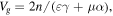
 ![${k}_{2}=\left(1/\beta n\right)\left[1/{V}_{g}^{2}-\alpha \gamma -\beta \left(\varepsilon \gamma \text{'}+\mu \alpha \text{'}\right)/4\pi \right]$](https://content.cld.iop.org/journals/1402-4896/91/2/025201/revision1/psaa0d62ieqn4a.gif) stands for the group-velocity dispersion (GVD). The value
stands for the group-velocity dispersion (GVD). The value  stands for the group-velocity dispersion (GVD), where
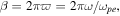
![$\alpha =\partial [\varpi \varepsilon (\varpi )]/\partial \varpi ,$](https://content.cld.iop.org/journals/1402-4896/91/2/025201/revision1/psaa0d62ieqn8.gif)
![$\alpha ^{\prime} ={\partial }^{2}[\varpi \varepsilon (\varpi )]/\partial {\varpi }^{2},$](https://content.cld.iop.org/journals/1402-4896/91/2/025201/revision1/psaa0d62ieqn9.gif)
![$\gamma =\partial [\varpi \mu (\varpi )]/\partial \varpi $](https://content.cld.iop.org/journals/1402-4896/91/2/025201/revision1/psaa0d62ieqn10.gif) and
and ![$\gamma ^{\prime} ={\partial }^{2}[\varpi \mu (\varpi )]/\partial {\varpi }^{2},$](https://content.cld.iop.org/journals/1402-4896/91/2/025201/revision1/psaa0d62ieqn11.gif) respectively. In equation (1),
respectively. In equation (1),  ,
, 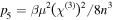 and
and ![${s}_{1}=({\chi }^{(3)}/2n)[\mu /{V}_{g}n-(\mu +\gamma )]$](https://content.cld.iop.org/journals/1402-4896/91/2/025201/revision1/psaa0d62ieqn14.gif) denote the cubic, pseudo-quintic nonlinearity and the SS effect, respectively. It is worth noting that all linear and nonlinear terms in equation (1) are related to the dispersive permeability
denote the cubic, pseudo-quintic nonlinearity and the SS effect, respectively. It is worth noting that all linear and nonlinear terms in equation (1) are related to the dispersive permeability  which is regarded as a constant
  in conventional materials because of weak magnetization [4]. It has been demonstrated that the dispersive permeability
  plays an important role in ultrashort pulse propagation, leading to the difference between MMs and conventional materials [17–19]. Moreover, these coefficients of the terms in equation (1) may be engineered by designing the unit structure of MMs. This implies that there are more possibilities for the existence of solitary waves in MMs [17]. The dispersive dielectric permittivity
  and magnetic permeability
  are described by the lossless Drude model
  and
and 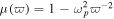 with
with  where
where  and
and  are the electric and magnetic plasma frequencies, respectively [17, 19]. For simplicity, here we neglect the losses since they may be reduced or compensated by introducing the gain and novel fabrication methods [37, 38]. Thus, for the typical value
  the refraction index
 ![$n=\pm {[\varepsilon (\varpi )\mu (\varpi )]}^{1/2}$](https://content.cld.iop.org/journals/1402-4896/91/2/025201/revision1/psaa0d62ieqn26.gif) is negative for
is negative for  and positive for
  According to the expressions of above parameters, for self-focusing nonlinearity,
  and
and  in the negative index region (NIR),
  and
and  in the positive index region (PIR); while for self-defocusing nonlinearity,
  and
and  in the NIR and
  and
and  in the PIR. Moreover, all the model parameters in equation (1) are the function of the normalized frequency
  whose specific dependence curves can be seen in figure 1 of reference [19]. Combined with the characteristics of these parameters, we will demonstrate that three new types of exact quasi-soliton solutions can exist in the anomalous dispersion regime of four regions of self-focusing and self-defocusing MMs. Hence for the convenience of our subsequent discussion, we define these four regions as Region I: in anomalous dispersion regime of self-focusing NIR; Region II: in anomalous dispersion regime of self-focusing PIR; Region III: in anomalous dispersion regime of self-defocusing NIR; Region IV: in anomalous dispersion regime of self-defocusing PIR. In general, equation (1) is not integrable, so we will seek new types of exact quasi-soliton solutions to equation (1) by ansatz method and investigate the formation conditions, the existence regions and the features of these solutions based on the parameter characteristics in MMs.

Figure 1. Distributions of the bright quasi-soliton (2) in (a) Region II (

 with
with 
 (b) Region IV (

 with
with 
 (c) Region III (

 with
with 
 respectively. Here soliton intensities are normalized by
  .
.
Download figure:
Standard image High-resolution image3. Exact quasi-soliton solutions and their characteristics
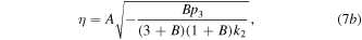
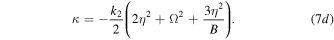
3.1. Bright quasi-soliton solution
Let us construct a bright quasi-soliton solution for equation (1) by assuming an ansatz:
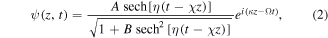
where  is related to the amplitude of quasi-soliton;

 and
and  stand for the inverse pulse, the frequency shift, the inverse group velocity and the wave number, respectively; and
  is a real constant larger than minus one. For
  the solution (2) can be simplified to a standard bright soliton
 ![$\psi (z,t)=A\;\mathrm{sech}[\eta (t-\chi z)]{e}^{i(\kappa z-{\rm{\Omega }}t)},$](https://content.cld.iop.org/journals/1402-4896/91/2/025201/revision1/psaa0d62ieqn64.gif) which has been studied in reference [39]. For
which has been studied in reference [39]. For  equation (2) is the form of a bright quasi-soliton. Substituting equation (2) into (1) and setting the coefficients of independent terms equal to zero, we can obtain five compatible equations. By solving these equations, we find when
  equation (1) admits the quasi-soliton solution in the form of equation (2) with the following parameters:
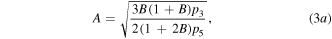


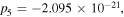
Here the frequency shift  is an arbitrary constant. From the equations (3a) and (3b), it is easy to see that the existence of the bright quasi-soliton (2) requires
 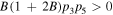 and
and 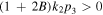 with the primary requirement
  Combined with the condition
  we find the bright quasi-soliton (2) may exist in three regions of self-focusing and defocusing nonlinear MMs, as shown in table 1. Obviously, the constant
  plays an important role in the existence regions of the bright quasi-soliton (2). This implies that the bright quasi-soliton can be formed in such three regions if we choose suitable
  Figures 1(a)–(c) present the distributions of the bright quasi-soliton (2) in the three existence regions, respectively. It is clear that in each existence region, the bright quasi-soliton (2) with different
  possesses different intensities and pulse widths that increase or decrease with the increasing of
  We notice that the quasi-solitons with different
  in each region have the same velocities because of the soliton velocity
  independent of
  In addition, the numerical confirmations of the analytical bright quasi-soliton (2) are depicted by circles, which well coincide with the analytical ones.
Table 1. Existence regions of the bright quasi-soliton (2) in self-focusing and defocusing MMs.
Ranges of 
|
Ranges of  , , and and 
|
Existence regions of bright quasi-soliton (2) |
|---|---|---|

|
  
|
Region II |

|
  
|
Region IV |

|
  
|
Region III |
3.2. Dark quasi-soliton solution
Similarly, we take an ansatz of dark quasi-soliton for equation (1) as follows:
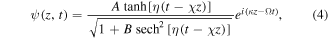
here 


 and
and  stand for the same soliton parameters as in the solution (2), respectively. The value of
  is still a real constant larger than minus one. For the special case
  the ansatz (4) is reduced to a standard dark soliton
 ![$\psi (z,t)=A\;\mathrm{tanh}[\eta (t-\chi z)]{e}^{i(\kappa z-{\rm{\Omega }}t)},$](https://content.cld.iop.org/journals/1402-4896/91/2/025201/revision1/psaa0d62ieqn102.gif) which has been studied in reference [19]; equation (4) with
which has been studied in reference [19]; equation (4) with  is the form of a dark quasi-soliton. Substituting equation (4) into (1) and solving the obtained six compatible equations, we find that when
  equation (1) admits the dark quasi-soliton solution in the form of equation (4) with the corresponding parameters as follows:
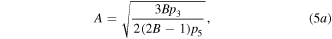


From the expressions of equations (5a) and (5b), it is easy to know that 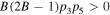 and
and 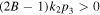 must be satisfied for the existence of the dark quasi-soliton (4). Combined the characteristics of model parameters with these conditions, it is found that the dark quasi-soliton (4) may also exist in three regions of self-focusing and defocusing MMs, as illustrated in table 2. Similar to the bright quasi-soliton (2),
  is an important parameter for the formation of the dark quasi-soliton (4), and has an impact on the intensity and pulse width of the quasi-soliton, while it has nothing to do with its velocity and wave number, which may be seen from equations (5a) and (5b). This means that the dark quasi-solitons with different
  in each existence region can propagate at the same velocities and different pulse widths when their intensities are normalized by
  as shown in figure 2. Furthermore, it is easy to infer that the dark quasi-solitons in different existence regions have different pulse widths and velocities because of different normalized frequencies corresponding to different parameters of dispersion and nonlinearity. Also, the numerical distributions in each existence region are in agreement with the analytical results, which can be seen in the corresponding figures with circles.
Table 2. Existence regions of the dark quasi-soliton (4) in self-focusing and defocusing MMs.
Ranges of 
|
Ranges of  , , and and 
|
Existence regions of dark quasi-soliton (4) |
|---|---|---|

|
  
|
Region II |

|
  
|
Region I |

|
  
|
Region III |

Figure 2. Distributions of the dark quasi-soliton (4) in (a) Region II (

 (b) Region I (

 with
with 
 and (c) Region III (

 Here the parameters in (a) and (c) are the same as those in figures 1(a) and (c) since they are in the same regions, and soliton intensities are normalized by
  .
.
Download figure:
Standard image High-resolution image3.3. Bright-grey quasi-soliton solution
Motivated by above bright and dark quasi-soliton solutions, we take another ansatz for equation (1) as follows:

where 


 and
and  still represent the same soliton parameters as in equations (2) and (4). The free constant
  is also required larger than minus one. For
  in this case, equation (6) is reduced to a plane wave. Different from the bright solution (2) and the dark solution (4), equation (6) may represent a bright quasi-soliton with an intensity
 ![${|\psi |}^{2}={A}^{2}/\{1+B{\mathrm{tanh}}^{2}[\eta (t-\chi z)]\}$](https://content.cld.iop.org/journals/1402-4896/91/2/025201/revision1/psaa0d62ieqn146.gif) for
for  or a grey quasi-soliton with an intensity
 ![${|\psi |}^{2}={A}^{2}/\{1-|B|{\mathrm{tanh}}^{2}[\eta (t-\chi z)]\}$](https://content.cld.iop.org/journals/1402-4896/91/2/025201/revision1/psaa0d62ieqn148.gif) for
for  That is to say, the quasi-soliton (6) is a bright soliton with a platform or a grey soliton with a nonzero dip for the case
  Following a similar solving process, we find that when
  equation (1) admits the quasi-soliton solution (6) with the parameters:

Similarly, the existence of the quasi-soliton (6) requires that  and
and  with
with  simultaneously. Considering the condition
  it is easy to find that the quasi-soliton (6) may exist in two regions and exhibit a bright or grey quasi-soliton form depending on the dispersion or nonlinearity, as well as the values of
  which are shown in table 3. The distributions of the quasi-soliton (6) in each region are presented in figure 3, respectively. Obviously, the bright ones have a platform in figure 3(a) and the grey ones have a nonzero dip in figure 3(b). Also, the quasi-solitons with different
  possess different platforms (backgrounds) and pulse widths for the bright (grey) form when we adopt normalized treatment
  These features can be seen clearly from figure 3. We also perform numerical experiments for the quasi-soliton (6) in each region, as correspondingly shown with circles in figures 3(a) and (b), which are in good agreement with the analytical prediction.
Table 3. Existence regions of the quasi-soliton (6) in self-focusing and defocusing MMs.
Ranges of 
|
Ranges of  , , and and 
|
Existence regions of quasi-soliton (6) | Intensity profiles |
|---|---|---|---|

|
  
|
Region III | Grey quasi-soliton |

|
  
|
Region II | Bright quasi-soliton |

Figure 3. Distributions of the quasi-soliton (6) in (a) Region II (

 and (b) Region III (

 The adopted parameters are the same as those in figures 1(a) and (c), respectively. Here the soliton intensities are normalized by
  .
.
Download figure:
Standard image High-resolution image4. The stability analysis
It should be mentioned that all three types of quasi-soliton solutions are obtained under the condition  corresponding to
  in NIR and
  in PIR for both self-focusing and self-defocusing MMs, respectively. However, the normalized frequency of incident pulses may fluctuate in real communication, resulting in nonzero SS parameter. On the other hand, solitons may be disturbed in the transmission by initial perturbation such as white noise, pulse width, etc. Therefore, it is necessary to investigate the stability of these quasi-solitons under the finite initial perturbation and nonzero SS parameter resulting from frequency fluctuation. Here we take the third type of quasi-soliton (6) as an example to investigate the stability by numerical simulation.
4.1. The stability under nonzero SS parameter
As mentioned above, the constant  is related to the background intensity of the quasi-soliton (6). Here we consider two cases: i) the stability under the same SS parameters and different constant
  as shown in figures 4(a) and (b); ii) the stability under the same constant
  and different SS parameters, as shown in figures 4(c) and (d). By comparing the curves in figure 4(a), we find that under the same SS parameters, the bright quasi-soliton with smaller
  can stably propagate keeping its shape unchanged after propagating 40
  As
As  is increasing, the bright quasi-soliton gradually broadens and then splits into two pulses. For the grey quasi-soliton, similar evolutions can be seen from figure 4(b), namely, with the increase of magnitude of
  it gradually evolves into two dips. In other words, the smaller the magnitude of
  the stabler its propagation. This means that when the SS parameter is nonzero, we can achieve stable bright and grey quasi-solitons by choosing suitable
  So we take
  for the bright form and
  for the grey form to discuss the stability under case ii); these are shown in figures 4(c) and (d), respectively. It can be seen clearly that the intensities of the bright ones are changed slightly under nonzero SS parameters corresponding to the frequency fluctuations
  and
and  and the intensities of the grey ones are affected more than those of the bright ones even if the incident frequency perturbations are small, i.e.
  and
and  This means that the grey quasi-soliton is more sensitive to the frequency fluctuation. So we can conclude that the quasi-soliton (6) may propagate stably by choosing suitable constant
  under nonzero SS parameters originating from the frequency fluctuation of the incident pulse.

Figure 4. Numerical evolutions of the quasi-soliton (6) under nonzero SS parameter. (a) Bright form in Region II with 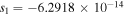 corresponding to
  and (b) grey form in Region III with
 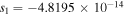 corresponding to
  under different
  Comparisons of the initial, exact and numerical evolutions of the quasi-soliton (6) in (c) bright form with
  and (d) grey form with
  after propagating 40
  under different SS parameters, corresponding to
  and
and  for bright ones and
  and
and  for grey ones, respectively.
Download figure:
Standard image High-resolution image4.2. The stability under pulse width fluctuation
We further investigate the stability of the quasi-soliton (6) under pulse width fluctuation. According to the results presented in figures 4(a) and (b), we still take  for bright form and
  for grey form. Figure 5 displays the numerical evolutions of the quasi-soliton (6) by adding a pulse width fluctuation of
  It can be seen from figures 5(a) and (b) that the features of the bright and grey quasi-solitons remain nearly unchanged after propagating 40
  except for slight changes in the intensities and pulse widths. This indicates that both the bright and the grey quasi-solitons can maintain their shapes unchanged under finite fluctuation of pulse width.

Figure 5. Numerical evolutions of the quasi-soliton (6) in (a) bright form in Region II with  and (b) grey form in Region III with
  under pulse width fluctuation of
  The insets show the comparisons of numerical simulations (red circle) and exact pulses (black solid line) after propagating 40
  Here, the adopted parameters are the same as those in figures 3(a) and (b), respectively.
Download figure:
Standard image High-resolution image
5. Conclusions and discussion
In conclusion, we have considered a generalized NLSE with dispersive permittivity and permeability describing the propagation of ultrashort pulses in MMs, and presented three new types of exact quasi-soliton solutions with a constant B by ansatz method. Based on the Drude model, we have investigated the existence regions and the characteristics of these solutions. It is found that by choosing suitable range of B, these bright and dark (grey) quasi-solitons can exist in wider regions in MMs than those in conventional materials. Also, as the constant B is also associated with the amplitude and the pulse width for each type of quasi-soliton, we may control the intensity and pulse width of the soliton by adjusting B. Such features imply that it is possible to form a quasi-soliton for an incident pulse with variable pulse width and intensity in MMs. As an example, we have numerically investigated the stability of the quasi-soliton (6) and found that the quasi-soliton (6) in both bright form and grey form can stably propagate under slight perturbations of nonzero SS parameter and the finite fluctuation of pulse width by choosing suitable B. The obtained results are important to explore much richer solitary waves in MMs. Finally, two things should be pointed out. i) Although the results we presented here are limited to theoretical analysis, we hope they may provide a theoretical reference for experimental verification in the future in view of the characteristics of artificial MMs, composed of various different unit structures, with tunable linear and nonlinear parameters. Moreover, the experiments and analytical approximation of practical NLTL MMs [33–36, 40] confirm that bright and dark envelope solitons can be observed and formed in the experiments. These results mean that MMs can be utilized to create suitable experimental circumstances for generating solitons [41]. ii) The results presented here are obtained without including the Raman effect. If the Raman effect is considered, there may not exist such exact solutions as presented above, and thus perturbation theory needs to be applied for the dynamics of bright and dark solitons [4, 42]. The characteristics of the above three types of bright and dark quasi-solitons under the perturbation of the Raman effect will be discussed in a separate paper.
Acknowledgments
This work is supported by the National Natural Science Foundation of China (NSFC) (grants 61178013, 61271160), and Selected Project of Overseas Science and Technology Activities of Shanxi Province (grant 201301).