


Abstract
An advanced adaptive control algorithm is used to study the control of external kink modes that are excited in the HBT-EP tokamak and have a natural toroidal rotation frequency near 8 kHz. The controller's system model is parametrized and the parameters are adjusted in real-time to match the measured plasma evolution. Depending upon a programmed phase angle, active feedback control is shown to either suppress or amplify the controlled amplitude by an amount comparable to the variations observed over a variety of plasma discharges. With negative feedback, the maximum amplitude is reduced to 40% of the uncontrolled value. With positive feedback, the amplitude increases to 155%. Intermediate feedback phases lead to an acceleration or deceleration of the mode rotation frequency in addition to changes in mode amplitude. As the feedback gain increases, the level of both mode suppression and mode amplification also increases. However, for sufficiently high gain, kink mode suppression becomes limited by the excitation of an additional, slowly rotating 1.4 kHz mode having the same helical structure as the uncontrolled kink. High gain amplification is limited by disruptive loss of plasma current. Experimental results are compared with numerical simulations based on a single helicity model, and qualitative agreement is found.
Export citation and abstract BibTeX RIS
1. Introduction
The control of magnetohydrodyamic (MHD) instabilities with active feedback is a promising technique for maintaining the plasma confinement in nuclear fusion systems with improved economic viability [1–3]. Development of advanced feedback algorithms has been shown to reduce the number of necessary sensors and actuators, as well as the required control power, without compromising feedback performance [4–9], which translates directly to simpler engineering and increased economic efficiency of any fusion plant.
The HBT-EP tokamak is designed to study the control of 3D MHD instabilities [10, 11]. A fast start-up (∼90 kA ms−1) followed by a current ramp of ∼2.5 kA ms−1 creates strong current gradients near the plasma edge, producing current-driven, external kink modes that are passively stabilized by a 10 × 2 grid of conducting, close-fitting, radially movable shell segments. Each shell segment holds two magnetic sensors and two magnetic control coils mounted over cutouts in the segments. The resulting 10 × 4 grid of sensors and control coil (see figure 1) is used for feedback control of MHD instabilities.

Figure 1. Sensors and control coils of the HBT-EP tokamak used in the presented feedback control experiments. The sensors (green) are mounted on the insides of 20 movable shell segments. Control coils (blue) covering 15° of toroidal angle are mounted on the outside of the segments, but a cutout ensures fast flux penetration.
Download figure:
Standard image High-resolution imageHBT-EP has pioneered the use of active magnetic feedback to control the resistive wall mode [12]. Recently, HBT-EP was equipped with a new control system that employs a graphics processing unit (GPU) for control computations [13]. The high computational resources of the GPU allowed the design of a novel control algorithm [14] that improves upon the previously used Kalman filter [7] by parametrizing the system model and deriving the parameters from the observed plasma evolution at runtime. This allows the control system to dynamically adapt to the stability properties of the evolving plasma equilibrium (which is especially important for a pulsed device like HBT-EP), and enables full compensation for both digital latency and multi-pole response of the analog actuators. The control algorithm, as well as the employed sensors and actuators, are described in more detail in Rath et al [14]. The algorithm tracks four rigidly rotating perturbations with toroidal mode number n = 1 at four different poloidal angles. The perturbations are treated as projections of one helical mode (with unspecified poloidal spectrum) that rotates with a slowly evolving frequency γ, which is a free parameter of the control system's plant model. At runtime, γ is determined by fitting the phase evolution to a constant rotation frequency over a continuously moving time window. By constraining the poloidal spectrum in time (by fitting to a toroidal rotation), but leaving it unconstrained in space, the same feedback algorithm is applicable to plasmas with differently shaped cross sections. The least-squares fit of the model parameters over a sliding window results in a slowly varying system model that is used to filter measurements and drive control coil currents so as to generate an external field with a fixed phase and amplitude relation to the perturbation. Depending on the phase, this results in suppression, excitation, acceleration or deceleration of the tracked perturbation.
This paper presents experimental results obtained with the new system and compares them with the predictions of a single-helicity model [15]. The paper is organized as follows. Section 2 describes the data analysis methods and includes an averaging method used to determine feedback performance over an ensemble of similar discharges. Section 3 presents the experimental results, showing suppression or amplification of the rotating kink mode as well as excitation of an additional low-frequency mode. Section 4 compares the experimental results with the predictions of the single-helicity model. Conclusions are summarized in section 5.
2. Data analysis
2.1. Automated shot selection
Figure 2 shows the typical evolution of an HBT-EP plasma. HBT-EP does not have facilities to dynamically adjust global plasma parameters during a shot. Instead, different kinds of shots are achieved by changing the voltage levels and triggering times of different capacitor banks. For this reason, the evolution of consecutive HBT-EP shots often differs significantly even when no adjustable parameters were changed. Therefore, analysis of feedback effects was carried out statistically by taking ensembles of shots, with the feedback parameters varying between ensembles, but not between individual shots of an ensemble. An automated selection algorithm was then run over the union of all ensembles to get a subset of shots with similar global parameters. After this elimination, the shots were repartitioned into ensembles with different parameters, and comparisons were done between ensemble averaged quantities.

Figure 2. Evolution of plasma parameters in two consecutive HBT-EP shots. Even though no controlled parameters are changed, the shot evolution differs considerably. In the first shot, a tearing mode arises briefly during start-up (2–3 ms), but changes the plasma evolution throughout the rest of the shot.
Download figure:
Standard image High-resolution imageThe selection algorithm works by first identifying the largest window of smooth plasma evolution in every shot, where a smooth evolution is defined by restrictions on the rate of change and value of plasma current, major radius and edge safety factor 'q'. For all further processing, attention is restricted to this window. After this, all shots are time shifted such that the edge safety factor peak (that occurs when the major radius hits 92 cm, see section 2.4) occurs at 5 ms. In the last step, the algorithm iteratively computes the average edge safety factor evolution and then drops the shot with the largest deviation from the average. This procedure is repeated until the standard deviation (averaged over time) of the remaining shots falls under 0.05.
Figures 3 and 4 illustrate the automatic selection procedure. The first figure shows the edge safety factor evolution of all shots taken for a specific set of experiments. All shots have already been time shifted. Since only regions of smooth plasma evolution are considered, the number of shots over which the average is computed changes over time and is indicated on the right axis. Figure 4 shows the subset of shots that are selected for analysis. Evidently, the standard deviation is significantly lower, and the total number of shots has dropped from about 60 to 33.
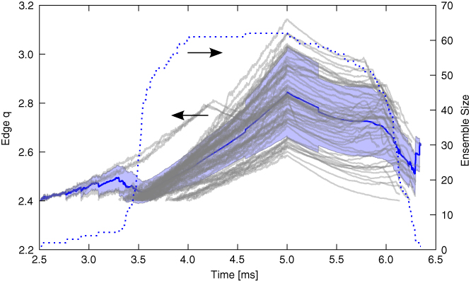
Figure 3. Edge safety factor (q) evolution of all shots taken for an experimental campaign. The blue line is the average, and the shaded region indicates one standard deviation. The dotted line indicates the number of shots that are contributing to the average at a given time.
Download figure:
Standard image High-resolution image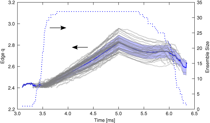
Figure 4. Edge safety factor (q) evolution of the shot subset from figure 3 that was selected for further analysis by the automated selection algorithm. The blue line is the average, and the shaded region indicates one standard deviation. The dotted line indicates the number of shots that are contributing to the average at a given time.
Download figure:
Standard image High-resolution image2.2. Signal separation
In order to analyse the effects of feedback control, sensor signals need to be separated into signals from the formally axisymmetric equilibrium fields and from the perturbations that are to be controlled. In theory, this can be done by reconstructing the axisymmetric equilibrium and then subtracting the sensor signals corresponding to this equilibrium. However, in practice this methods is not feasible due to finite sensor alignment accuracy. Because of the order-of-magnitude differences between the equilibrium and perturbed signals, even a slight misalignment of a sensor can result in some components of the equilibrium field being treated as perturbations of a magnitude that completely shadow the true perturbed signal. Instead, signals have therefore been separated using biorthogonal decomposition (BD) [16, 17].
Consider a set of sensors xi that take measurements at discrete time points tj. Let the measurements carried out by a single sensor at different times be written as a row vector, and the matrix formed by stacking the row vectors of the different sensors be X, so that Xij = xi(tj). While not necessary for the BD in the general case, for the purpose of this paper all measurements were zero centred, so that ∑jxi(tj) = 0. The singular value decomposition (SVD) U. S. V† of X is called a BD, and the columns of U and V (or rows of V†) are called spatial and temporal modes respectively.
The significance of these modes can be understood as follows. By the definition of the SVD, the columns of U are orthonormal and eigenvectors of X.X† with eigenvalues
 . Now consider the elements of the X.X† matrix:

Since ∑jxi(tj) = 0, the elements of X.X† are the correlation coefficients between the different sensors. Consider now a hypothetical second set of sensors yi(tj) where each sensor measures a linear combination of the real sensors:

Since the columns of U are eigenvectors of X.X†, the fictitious sensors yi will be uncorrelated in time. Also, by virtue of being linear combinations of the real sensors, every sensor yi measures a spatially distributed structure that has an amplitude Uji at the position of the real sensor j. In other words, the measurements xi can be understood as being generated by the independent time evolution of different static spatial structures Uji—the spatial modes. The singular value of a mode is proportional to the overall amplitude of the mode and gives a measure of how much a given mode affects the measurements over time.
BD thus decomposes a set of measurements from different points in space and time into a superposition of spatially invariant and temporally uncorrelated modes. This makes the BD well suited to compute the equilibrium components in a set of sensor signals: even if the individual sensors are not perfectly aligned, the equilibrium field must result in highly correlated signals with a distinct, invariant spatial structure. This means that those structures have a very high chance of being isolated as individual modes when performing a BD of measurements over the plasma lifetime. To determine the equilibrium components in a set of sensor measurements, we therefore decompose the measurements into spatial and temporal modes using BD, identify the modes corresponding to equilibrium signals, and then reconstruct the signals from just these modes.
Equilibrium spatial modes are identified by their toroidal variation, which is expected to be due to sensor misalignments only, and thus restricted to a few per cent of the average value. Perturbed modes, on the other hand, may not be axisymmetric and thus have toroidal variations as large as the individual sensor signals. Equilibrium signals also have higher amplitudes, so equilibrium modes are expected to have larger singular values than perturbed modes and the search for equilibrium modes can be stopped as soon as the first perturbed mode is found.
Figure 5 illustrates the toroidal profiles of the first five spatial modes in a sample shot. Here the equilibrium components are isolated in the first four modes (which show toroidal variation only due to different sensor orientations), while the fifth mode is generated by an n = 1 perturbation. The poloidal profiles (not shown) allow further classification of the equilibrium modes into uniform horizontal displacement and vertical stretching/compression.
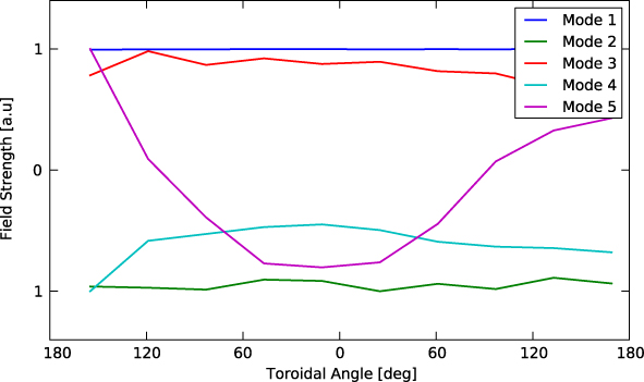
Figure 5. Toroidal profiles of the spatial BD modes in the bottom sensor array. From the relative magnitude of the variation, the first four modes can clearly be identified as equilibrium modes.
Download figure:
Standard image High-resolution imageFigure 6 shows an individual sensor signal and its equilibrium component as determined by BD. When used this way, the BD thus acts similar to a low-pass filter. However, instead of filtering every signal separately, all signals are processed together, taking into account their spatial relations. Figure 7 illustrates the shape of the perturbation that remains after subtraction of the equilibrium fields using a density plot of the magnetic field strength at different times and poloidal positions. As one can see, perturbations take the form of coherent, rotating modes.
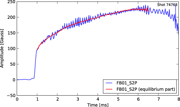
Figure 6. A typical poloidal sensor signal in an HBT-EP discharge and its equilibrium component as determined by BD.
Download figure:
Standard image High-resolution image
Figure 7. Perturbation amplitudes in a poloidal sensor array. The fluctuations are on the order of 12 G. The equilibrium components of the signals are subtracted using BD. Blue dots represent sensor locations
Download figure:
Standard image High-resolution image2.3. Frequency spectra
In HBT-EP, perturbation amplitudes typically fluctuate around a saturated value, resulting in large apparent standard deviations when averaging in the time domain. Effects of the feedback control system are therefore best observed in frequency space. The (complex) spectral amplitude f(ω) of a mode that has measured (real) amplitudes Ac(t) and As(t) for its cosine and sine components, respectively, is defined as

where
 denotes the Fourier transform. With this definition, |f(ω)| gives the amplitude of the mode at frequency ω, and arg(f(ω)) gives a phase offset. Spectral plots in this paper show the shot-averaged |f(ω)| in a solid line, and a shaded band indicates the standard deviation. Spectral amplitudes are plotted in units of tesla and have magnitudes of several kilo-gauss. To prevent confusion with the time domain signal (which is in the order of tens of gauss) frequency domain amplitudes are labelled simply as 'amplitude' without an explicit unit in this paper.
It should be noted that f(ω) ≠ f(−ω)* (with the asterisk indicating complex conjugation), because the input to the Fourier transform is complex. For an idealized mode that rotates at a fixed frequency ω0, f(ω) = δ(ω ± ω0), and the sign distinguishes between the directions of rotation.
2.4. Geometric coupling intervals
An important feature of HBT-EP plasmas is the relationship between plasma major radius and plasma minor radius. As illustrated in figure 8, the upper and lower limiters limit the maximum minor radius of HBT-EP plasmas to 15 cm. However, due to the inner and outer limiters, the maximal minor radius can only be achieved when the plasma centre (major radius) is between 90 and 92 cm. For major radii above 92 cm, the plasma becomes outboard limited, and the minor radius decreases linearly with increasing major radius.

Figure 8. Location of feedback sensors relative to the plasma surface. The control coils are at the same poloidal locations as the sensors but toroidally behind. For plasma major radii above 92 cm, the plasma surface recedes from the lower and upper sensors and coils.
Download figure:
Standard image High-resolution imageTypical HBT-EP plasmas start out outboard limited with a small minor radius, then grow to the maximum of 15 cm, and typically disrupt around the time that the major radius hits 89 cm. This is reflected in the edge safety factor profile of the second shot in figure 2. The edge q starts to rise at 3 ms (because the rising minor radius dominates over the effects of the increasing plasma current), reaches a peak at 6.3 ms (when the minor radius becomes constant) and then falls again (because the plasma current continues to rise).
As can be seen from figure 8, with falling minor radius the plasma couples less to the upper and lower feedback sensors and control coils. The interaction between the plasma and the control system is therefore fundamentally different for major radii above and below 92 cm. The time period between activation of the feedback system and the major radius crossing 92 cm from above will be called the 'weak coupling interval'. The time period between crossing of 92 and 90 cm (or plasma disruption, whatever happens earlier) will be called the 'strong coupling interval'. When analysing data, these periods were treated separately, i.e. frequency spectra were calculated separately for each period of every shot.
3. Experimental results
3.1. Recap of previous results
In order to put the new results of this paper into context, this section briefly reviews the initial findings that were reported in Rath et al [14].
For constant feedback gain, it was found that mode amplitude in the strong coupling interval could be suppressed to 40%, from an uncontrolled amplitude of 0.2 to a controlled amplitude of 0.08. However, at the same time an additional slow −1.4 kHz mode was excited to an amplitude of 0.09. Changing the feedback phase by 180° was expected to amplify the perturbation, but instead resulted only in an increased deviation between shots with no change in the average mode amplitude of 0.2. This is illustrated in figure 9. Intermediate feedback phases resulted in a combination of suppression and acceleration or deceleration of the rotation frequency, as shown in figure 10.
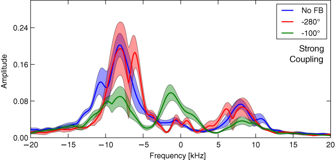
Figure 9. Frequency spectrum of magnetic perturbations without feedback, and with feedback at the −100° and −280° phases in strong coupling interval. At −100°, the amplitude of the −8 kHz mode is suppressed to 40% (from 0.2 to 0.08), but an additional −1.4 kHz mode is excited. At −280°, no significant amplification is observed, but shot-to-shot variability increases by a factor of two and a new mode is excited at −6 kHz. Figure reproduced with permission from Rath et al [14]. © 2013 IOP Publishing.
Download figure:
Standard image High-resolution image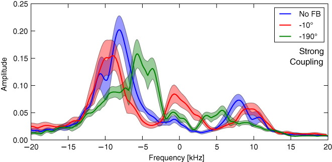
Figure 10. Effects of −10° and −190° phased feedback compared to the no-feedback case in the strong coupling interval. Both phases suppress the dominant −8 kHz mode, but suppression is not as strong as for the −100° feedback shown in figure 9. However, −10° and −190° phasing results in an additional acceleration and deceleration of the mode rotation frequency respectively. Figure reproduced with permission from Rath et al [14]. © 2013 IOP Publishing.
Download figure:
Standard image High-resolution image3.2. Phase dependence with weak coupling
Figure 11 shows the frequency spectrum for different feedback phases calculated over the weak coupling period. In contrast to figure 9, the uncontrolled amplitude of the dominant mode is about 55% lower (0.11 versus 0.20), and the mode rotates slightly faster at −10 kHz. Also, in the weak coupling period, feedback at 280° is able to amplify the dominant mode to 0.17 (with some shots reaching 0.20), i.e. to the uncontrolled amplitude in the strong coupling period. Additionally, the mode rotation is slowed down to −7 kHz. In contrast, attempts to suppress the mode with 100° feedback result in a barely significant reduction from 0.11 to 0.10, i.e. to the same level to which the mode was suppressed in the strong coupling period. In both the strong and weak periods, suppression of the mode is accompanied by excitation of an additional slow mode (with the amplitude of the slow mode coinciding with the maximum amplitude reached by the −8 kHz mode under feedback amplification).
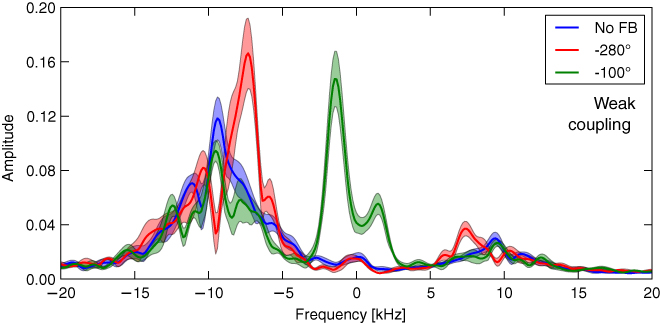
Figure 11. Frequency spectrum of magnetic perturbations without feedback, and with feedback at the −100° and −280° phases in the weak coupling period. At −100°, suppression of the dominant −8 kHz mode is barely significant, but a strong −1.4 kHz mode is excited. At −280°, the amplitude of the dominant is amplified by 55% from 0.11 to 0.17, and rotation frequency reduced from −10 to −7 kHz.
Download figure:
Standard image High-resolution imageIt should be noted that the reduced mode amplitude in the weak coupling period is not a direct consequence of the reduced coupling between upper and lower feedback sensors and the plasma. The direct effects of the reduced coupling can be seen when comparing the mode amplitudes measured using only the upper/lower and only the midplane sensor arrays and is only about 15%. The observed amplitude drop of 55% between the different coupling periods must thus be caused by additional changes in plasma response or saturation mechanism.
3.3. Gain dependence
The feedback experiments shown in figures 9–11 were carried out with a gain arbitrarily chosen to use about 50% of the available control power (corresponding to fields of about 30 G at the plasma surface). To quantify the effect of different gains, a second set of experiments was performed with varying gain and constant, suppressing phase. The results are highlighted in figures 12 and 13. Both figures show the frequency spectrum of the lowest tested gain, the highest gain that could be applied without causing a plasma disruption, and the no-feedback case. Gains are normalized to 20 A of control coil current per tesla of mode amplitude at −8 kHz rotation. The lowest gain of 144 then corresponds to fields of about 5 G at the plasma surface. Figure 12 shows the spectrum for different gains during the strong coupling period, and figure 13 during the weak coupling period.
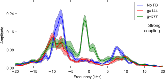
Figure 12. Mode spectrum for different feedback gains in strong coupling period. Reducing the gain from 544 to 144 does not change suppression, but prevents excitation of the slow −1.4 kHz mode. Further reductions in gain reduce suppression as expected.
Download figure:
Standard image High-resolution image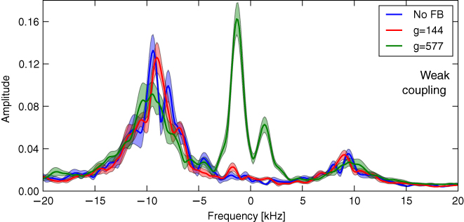
Figure 13. Mode spectrum for different feedback gains in the weak coupling period. Raising the gain excites an additional slow mode, but suppression of the dominant mode is limited to the amplitude that was achieved with strong coupling.
Download figure:
Standard image High-resolution imageAs one can see, in both cases there is a wide range of feedback gains that result in approximately the same suppression. In this range, larger gains only marginally improve suppression, but instead excite an additional slow mode to increasing amplitudes. The excitation is most likely the reason for the lack of further increases in suppression of the dominant mode because it invalidates the control algorithm's assumption of rigid rotation at constant frequency (fast and slow mode have the same spatial structure).
Just as observed in the phase scan, the gain scan indicates that the amplitude of the dominant, rotating mode can be controlled in between a minimum and maximum amplitude. In the weak coupling period, the natural amplitude of 0.13 can be decreased to 0.12 using feedback control (or to 0.09 at the price of exciting an additional mode). In the strong coupling period, the natural amplitude of 0.23 can be suppressed down to 0.09 (without exciting an additional mode). While a gain scan at positive feedback phase has not been performed, it is expected that lower gain will not result in stronger amplification, so figures 9 and 13 establish the upper limit on mode amplitude. In the strong coupling period, mode amplitudes are already saturated at 0.20 and cannot be amplified further, while in the weak coupling period the natural amplitude of 0.12 can be amplified to a saturated amplitude between 0.17 and 0.20 (depending on the shot).
4. Comparison with simulations
4.1. Model
In HBT-EP, single-helicity kink dynamics during active feedback control can be modelled with a formalism that combines Boozer's general prescription for the coupling of currents in external conductors to the plasma [18–20] and the equations for the external kink in the presence of viscous dissipation developed by Fitzpatrick and Aydemir [21, 22]. The use of single-helicity dynamics with relatively high levels of plasma dissipation was described in Mauel et al [15] and was shown to describe the plasma's time-response to the application of 'phase-flip' resonant magnetic perturbations (RMPs) [23, 24].
In this model, kink dynamics are represented by the evolution of the total perturbed flux at the plasma surface, ψa(t) and at the wall, ψw(t). The resonant component of the control–coil flux, ψc(t), is related to the control–coil current by ψc = McIc. The dynamical quantities are complex and can be related to the physical observables by multiplying with the assumed helicity of the mode and taking the real part. The perturbed wall flux at poloidal angle θ and toroidal angle φ, for example, is ℜ{ψw exp[i(mθ − nφ)]}.
In the presence of plasma rotation and high plasma dissipation [15], the combined single-helicity dynamics of the plasma, wall, and control coils are described by a linear system,
An explanation of the various parameters and their values is given in table 1 and in Mauel et al [15]. The plasma–wall coupling parameter, c, and wall eddy current dissipation rate, γw, are computed with the VALEN code [25] using MHD plasma equilibria consistent with experimental measurements. When the current in the external control coils are set to zero, the unforced response of the coupled plasma–wall system is a combination of two normal modes, which differ in the complex ratio, ψa/ψw. When the mode rotation is sufficiently fast compared with the wall time, |Ω| ≫ γw, these modes are called the wall-stabilized kink mode and the slow wall mode. The wall-stabilized kink mode has a complex growth rate
 . The slow wall mode is stabilized by plasma rotation and decays at a rate
![$\gamma \sim \gamma_{\rm w}/(1-c) \times [1/(1- \bar{s} + \rmi\bar{\alpha}) - 1]$](https://content.cld.iop.org/journals/0029-5515/53/7/073052/revision1/nf468405ieqn004.gif) . The relevance of this parametrization of kink dynamics in HBT-EP has been shown previously [23, 24] by fitting values for
. The relevance of this parametrization of kink dynamics in HBT-EP has been shown previously [23, 24] by fitting values for
 to the measured time evolution of the (m, n) = (3, 1) kink mode.
Table 1. Parameters of the (m, n) = (3, 1), single-helicity model used for numerical modelilng of kink mode interactions with resistive wall segments and control coils [23].
| Parameter | Description |
|---|---|
| ψa | Complex amplitude of perturbed poloidal flux at the plasma surface |
| ψw | Perturbed poloidal flux at the wall |
| ψc | Resonant helical flux at the wall due to control coils |
| Ω/2π ≈ −8 kHz | Toroidal mode rotation frequency (in electron drift direction) |
| γr = 22 ms−1 | Growth rate of kink mode with viscous dissipation |
| γw = 3.4 ms−1 | Eddy current decay time of the wall (from VALEN [25]) |
| c = 0.261 | Plasma–wall coupling coefficient (from VALEN [25]) |
| cf = 0.8e−iπ/10 | 'Mode control' coupling parameter for control coils, including phase |
 |
Normalized kink stability parameter,
 corresponds to the ideal wall limit corresponds to the ideal wall limit |
 |
Normalized viscous torque parameter, −Ω/γr |
| Lc = 91 µH | Measured self-inductance of each 12-turn control coil |
| Rc = 1.0 Ω | Measured resistance of each control coil |
| Mc = 2.3 µH | Mutual coupling between control coils and resonant wall flux |
When closed-loop magnetic feedback is applied, the control flux ψc(t) = McIc(t) evolves in time, and equation (4) must be combined with the voltage–current relationship for the control coils. Using measurements of the self-inductance and resistance of the control coils, the control flux evolves in time as

The complex parameter Hc is added to represent relatively small, frequency-dependent shifts in the mutual inductance, Mc, determined by detailed measurements made in situ without plasma.
The results reported here applied a voltage, V(t), in proportion to the product of a complex, linear gain, geiδ, with the helical perturbation of the poloidal field measured just inside the wall segments. The sensors are displaced 18° toroidally from the control coils, and this results in a small phase-shift to the mode-coupling parameter, cf, shown in table 1. The perturbed poloidal field δBp measured by a wall-mounted sensor depends on the perturbed helical flux at both the plasma surface and the wall,

The resulting closed-loop system is third order and is characterized by three roots parametrized by the complex proportional gain, geiδ. Stability occurs when the gain is adjusted so that all three roots have their real parts less than zero, ℜ(γ) < 0. As the magnitude and phase of the gain change, so do the locations of the three linear roots in the complex γ-plane.
Figure 14 shows the three roots of the closed-loop system for a range of proportional gains, geiδ. When the programmed feedback phase is adjusted to stabilize the rotating wall-stabilized kink mode, the mode's damping rate increases with increasing gain. In the limit of the gain g going to zero, the two low-frequency modes decouple into a wall mode (ψw/(ψa + ψc) ≫ 1, γ ≈ γw/(1 − c)), and the control coil mode (ψc/(ψa + ψw) ≫ 1, γ ≈ −Rc/Lc). As the closed-loop gain increases, these modes couple. For sufficiently high gain, g ∼ 500 V/T−1, the low-frequency mode becomes unstable for the same programmed feedback phase that leads to stability for the rotating kink mode.

Figure 14. Loci of the three roots of the closed-loop system model for single-helicity kink modes in HBT-EP. The magnitude of the proportional gain takes values from g = 50, 100, 250 and 500 V/T−1. For each gain magnitude, the feedback phase angle varied from 0 < δ < 2π. The optimum phase angle, δ = −100°, is shown in green.
Download figure:
Standard image High-resolution imageMore realistic modelling of the closed-loop system can be performed by a time-sampled discretization of the third-order closed-loop system. We use a sampling period of 4 µs and a zero-order hold approximation for the voltage applied to the distributed array of control coils, i.e. the discrete system is exact if the voltage updates instantaneously every 4 µs. The control output voltage at the nth sample V[n] is then related to digitized poloidal field δBp[n − 4] 4 samples earlier to take into account 16 µs of processing latency using the feedback law

Simulations of the discretized closed-loop system were performed without artificial noise, so that the growth rates and rotation frequencies for different feedback phases δ and feedback gains g could be computed by eigenvalue analysis. With g and δ fixed, any solution is either exponentially growing or decaying at a fixed rate, and rotating at a fixed frequency. In contrast, the experimentally observed perturbations are fluctuating in time around a saturated amplitude, and rotate at time-varying frequencies. For this reason, the comparison between simulation results and experiments are necessarily qualitative rather than quantitative. In the experiment, we observe changes in the average mode amplitude and fluctuation spectrum upon application of feedback control. In the simulations, we look at changes in the linear growth rate and rotation freqency. Although the physical mechanism responsible for amplitude saturation is not yet fully understood, it is assumed that less stable modes can achieve larger saturated amplitudes, and more stable modes can only reach smaller saturated amplitudes.
4.2. Simulation results
Figures 15, 16 and 17 show the effects of feedback at values of g and δ on the eigenvalues of the closed system including digital latency. The simulations always result in one rapidly rotating mode (≈ − 8 kHz, plotted in green) and two slowly rotating modes (plotted blue and red), which correspond to the slowly rotating wall and control-coil modes coupled by feedback. Dotted lines indicate the growth rates and rotation frequencies in the absence of feedback, g = 0. In figure 15, when g ∼ 100, optimum feedback suppression of the wall-stabilized kink occurs with a feedback phase, δ = −100°. Figure 16 shows the deviation of the frequency from its mean value to make the relative changes in frequency for different feedback phases more clear. Figure 17 shows the growth rates for increasing feedback gain at a feedback phase of −100°.
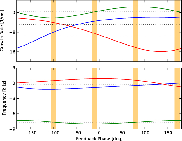
Figure 15. Simulated growth rates (top) and mode rotation frequencies (bottom) for different feedback phases at fixed gain, g = 100. Dotted lines indicate the growth rate and frequency in the absence of feedback. Shaded regions indicate the phases that are tested experimentally.
Download figure:
Standard image High-resolution image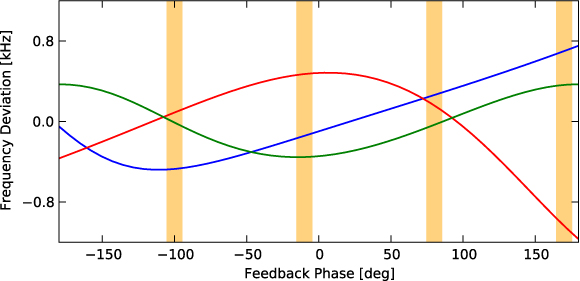
Figure 16. Relative changes in rotation frequency for different feedback phases, compared to the average over all feedback phases. (Simulation results, shaded regions indicate the phases that are tested experimentally.)
Download figure:
Standard image High-resolution image
Figure 17. Simulated growth rates and rotation frequencies with different feedback gains at the −100° phase.
Download figure:
Standard image High-resolution image
From the figures, the following experimental observations are found to be correctly predicted by the model:
- At −100° phase, the fast mode is suppressed and its rotation frequency is unchanged. A slow, co-rotating mode is being amplified without changes in rotation frequency, but with low gain does not cross the threshold to instability.
- At the −280°/80° phase, the fast mode is amplified, and no co-rotating mode is excited.
- At the −10° phase, the fast mode amplitude is in between the −100° and −280° case, and the mode rotation frequency is increased. A slow, co-rotating mode is amplified with a frequency slightly lower than at the −100° phase.
- At the −190°/170° phase, the fast mode amplitude is in between the −100° and −280° case, and the mode rotation frequency is decreased. The co-rotating slow mode is suppressed.
- With increasing feedback gain at the −100° and −10° phases, the fast mode is increasingly suppressed and co-rotating slow modes become increasingly amplified. At some gain threshold, the slow mode becomes unstable and suppression of the fast mode levels out.
The discretized simulation with latency also predicts excitation of a second slow, counter-rotating mode with increasing gain that has not been observed in experiments. This may be a consequence of using a high-pass filter [14] for real-time signal separation in the control system that has not been included in the model. Since the counter-rotating mode has the lowest frequencies, it may be invisible to the control system, and thus never get excited.
It should also be noted that there is one aspect in which the model's predictions do not fully match the experimental observations. At the amplifying (80°/−280°) phase, the model predicts mode amplification at unchanged frequency, but experimental results indicate amplification accompanied by a reduction in frequency. The reason for this effect is not yet clear.
5. Summary and discussion
A new feedback control algorithm was tested experimentally at HBT-EP. The algorithm, presented in more detail in Rath et al [14], continuously updates its system model by least-squares fitting of the measurements over a moving time window.
Without feedback control, plasma behaviour in HBT-EP is dominated by a saturated (m, n) = (3, 1) mode rotating near −8 kHz. The saturated amplitude in the absence of feedback control varies by a factor of two (between 1 and 2 mT peak amplitude), depending on plasma major radius and edge safety factor. With active feedback control, the saturated mode amplitude is consistently amplified to 2 mT or suppressed to 0.8 mT. These upper and lower limits are independent of the uncontrolled amplitude. Positive feedback, when applied at a time where the uncontrolled amplitude has already reached 2 mT will not result in any amplification, but negative feedback at this time always decreases the amplitude by approximately 60%. Similarly, positive feedback at a time where the uncontrolled amplitude is 1 mT amplifies the mode to up to 2 mT, but negative feedback decreases the amplitude only slightly to 0.8 mT.
When feedback gain is further increased after an amplitude limit is reached, the plasma either disrupts (in the case of positive feedback) or forms an additional mode with the same spatial structure that rotates at a significantly lower frequency (∼−1.4 kHz).
The effects of feedback gain and phase on mode amplitude and frequency, and especially also the excitation of an additional slow mode, are well captured by a single-helicity model based on the Fitzpatrick–Aydemir equations in the high plasma dissipation limit [15]. Numerical simulations, including digital latency, qualitatively reproduce the experimental observations, with the only exception being a frequency reduction at the amplifying phase that was observed in experiments but not predicted by theory.
5.1. Implications and future research
It has been reported before [6, 26] that with increasing beta, control of multiple, spatially different modes ('multi-mode control') becomes important. The wider implications of the results presented in this paper are that multi-mode effects may also take the shape of a single spatial perturbation with a non-trivial, multi-frequency time evolution. As we have shown, the presence of such multi-mode phenomena may impair even a control algorithm explicitly designed for multi-mode control (in terms of spatially distinct modes) and thereby establish a lower limit on the amplitude to which a perturbation can be suppressed.
Future research on HBT-EP will extend the control system to simultaneous control of multiple modes differing not in their spatial but temporal profile to evaluate whether this will allow a further decrease in the perturbation amplitude. Theoretical considerations [27] indicate that one way to achieve this may be to combine measurements from both poloidal and radial wall-mounted sensors. Adding additional terms proportional to the perturbed radial field to the control output voltage may enable robust stabilization of both the rapidly rotating wall-stabilized kink and the lower-frequency, rotationally stabilized wall mode at high gain.
The experiments presented in this paper also represent the first successful testing of a GPU-based, microsecond latency control system in the field of plasma physics. The short development cycles, large computational resources and large number of input and output channels of this system have proved to be an ideal platform for developing and running advanced feedback algorithms.
Finally, the use of BD to separate magnetic measurements into perturbed and equilibrium components has been shown to be a valuable analysis tool. In contrast to toroidal averaging or low-pass filtering, the combination of spatial and temporal information in the BD correctly handles both toroidal asymmetries due to sensor alignment errors (which would appear as perturbations when using toroidal averaging), and low-frequency modes (which would appear as equilibrium signals when performing temporal filtering).