

Abstract
Sedimentation of colloids is a common phenomenon in various industrial processes. Aggregation of nanoparticles is expected to occur during the processes. However, previous studies often ignore the important features of aggregates, e.g. porosity and possible seepage, leading to a mathematical description of the sedimentation processes of low reliability. In this study, we successfully elaborated the partial differential equation of the dynamic concentration distribution of regimented colloids based on the Stokes approximation and diffusion along the negative gradient of concentration. The permeability of aggregates was obtained by the finite volume method and the ratios of the velocities of flowing around (uf) to seepage through (us) aggregates over various primary particle sizes and aggregation structures were obtained based on the Darcy equations. After validation of the model, the effects of size and density of the particles and aggregates on the concentration profiles were investigated. Our results indicate that both an increase in size and density of particles and aggregates can accelerate the sedimentation process, and lead to more 'thorough' sedimentation. We mathematically explain why suspensions with high particle concentration are more unstable. What is more, replacing gravity with other volume forces, e.g. centrifugal force and magnetic forces, our model is expected to be applicable to centrifugation or magnetic sedimentation processes.
Export citation and abstract BibTeX RIS
1. Introduction
The aggregation and sedimentation of suspended particles play a major role in the ecology and pollution of environmental systems [1–3]. In particular, for small particle suspensions (diameter < 100 nm), also called colloids, aggregation and sedimentation significantly affect chemical reactions, heat transfer and other industrial processes such as centrifugation or magnetic sedimentation [4–8].
Previous studies on the sedimentation processes of colloids [6, 7] indicate that the sedimentation velocity significantly depends on the size and surface coating of particles. In fact, the sedimentation velocity of particles is affected by settling along gravity, centrifugal forces or magnetic field forces, and diffusion along the negative concentration gradient. The settling of small particles along gravity or other volume forces can be described by Stokes's approximation when Re is much less than 1. Kim et al [8] have investigated in detail the way in which gravity affects the gelation of adhesive colloidal particles. This is an important example that illustrates the competition between Brownian diffusion and phase separation enhanced by gravitational settling in the gelation process of adhesive hard spheres, and they found that both intermolecular forces and gravity force might change the phase behavior of the suspension and lead to aggregation of primary particles. If aggregation occurs, the sedimentation process becomes very complex. Some classical kinetics of colloid theories point out that nanoparticles, due to their large specific surface area, do not subside in the presence of gravity alone due to their random movement driven by Brownian motion [9, 10]. However, lots of experimental results have shown different phenomena. Due to their high speed and random movement, nanoparticles always collide with each other. The collisions will often lead to formation of aggregates or clusters, considering that a large proportion of collisions are inelastic collisions due to Van der Waals forces [1, 11–15]. The fluid dynamics of aggregates has been studied in previous work [16, 17]. Gastaldi et al [16] applied the reflection method to calculate the drag force on each monomer, and they found that the stress state and motion of aggregates are closely related to their structure. Seto et al [17] evaluated the hydrodynamic interaction acting on rigid fractal aggregates in an imposed shear flow using Stokesian dynamics. Their study explained why the stress acting on an aggregate and moments of the forces acting on contact points among particles follow power-law behaviors with the aggregate size. However, rare research has considered the porosity of the aggregate, which is expected to have a significant effect on the motion of the aggregate.
The porosity of the aggregate increases the complexity of its motion in base liquid. Generally, the sedimentation processes of aggregates are very slow, typically only several centimeters after several days. It is thus assumed that base fluid, as shown in figure 1, may both seep (base fluid seeps into the holes in the bottom of aggregates and out of the holes in the top of aggregates, like the seepage in porous media) and flow around (base fluid bypasses aggregates along their surfaces) aggregates in the process of sedimentation. Previous studies [18–20] investigating sedimentation of aggregates have always ignored the porosity and possible seepage of aggregates. In our study, the porosity and the resultant seepage of aggregates have been especially considered.
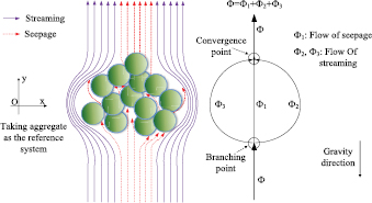
Figure 1. Left: sketches of the flow field of an aggregate in the subsiding process. Because the aggregate is deemed to be a reference system, the sedimentation of an aggregate corresponds to a base fluid seeping through and flowing around the aggregate. Right: separating flow induced by seepage of a porous aggregate.
Download figure:
Standard image High-resolution imageIn order to determine whether seepage exists, the porosity and permeability of aggregates should first be obtained. Many previous studies [21–29] have investigated the permeability of periodic arrays of spheres, cylinders, microchannels, fractured porous media, self-affine aperture fields, etc using the finite element method, the lattice-gas cellular automaton method, or other flow mechanics theories in two or 3D cases. In our study, particles are assumed to be spheres, thus aggregates are arrays of spheres. Unlike common seepage, where base fluid can only seep through a porous media, base fluid can either seep through or flow around the aggregates they encounter. Therefore, another key problem is to find the flow distribution, i.e. the proportions of flows of streaming and seepage.
The theoretical model for our consideration will be given in section 2. In section 2.1, we will build a basic model about the sedimentation of monodispersed and non-osmotic particles in suspension based on gravity setting and concentration diffusion. In section 2.2, we deduce the relation of the velocities of flow around and seeping through an aggregate by analogy with parallel pipes and parallel circuits. In section 3, the results of two models are discussed. What is more, the permeability of aggregates is studied using a finite volume method, and finally the main conclusions are given in section 4.
2. Theoretical models
2.1. Simplified model: sedimentation of monodisperse and non-osmotic particles in suspension
For monodisperse and non-osmotic particles without considering interactions among the particles (including aggregation processes), the primary forces acting on each particle are gravity, buoyancy, resistance and Brownian force. For a typical case that the density of particles is larger than the base fluid, i.e. gravity is larger than buoyancy, particles settle due to gravity. Assuming that suspended particles are very small, the Re (Re = ua/ν, where u is the sedimentation velocity, m s−1, a is the diameter of the particles, and m and ν are the kinematic viscosity, m2 s−1) will be much less than 1, thus Stokes's approximation can be applied as

where ut is the sedimentation velocity at t = ∞, g is gravitational acceleration, m s−2, and μ = νρb is the dynamic viscosity coefficient of the base fluid, kg (m s)−1. In fact, the sedimentation velocity u always reaches ut very quickly (less than 0.01 s), thus we ignore the short-lived unsteady accelerated flow and assume u = ut in the sedimentation process.
On the other hand, the macroscopic effect of the Brownian force is diffusion, i.e. particles directionally move from high to low concentration regions, which can be shown as
where dm is the differential mass of the solute, kg, D the diffusion coefficient, m2 s−1, A the cross sectional area of mass diffusion, m2, c the concentration, kg m−3, x the direction perpendicular to A, m, and dt is the differential time, s. Equation (2) indicates that the migration rate of the particles is proportional to the gradient of concentration and diffusion coefficient D. For spherical and homogeneous particles, the diffusion coefficient can be obtained by
where T is the temperature, K, kB the Boltzmann constant, J K−1, μ the dynamic viscosity coefficient of base fluid, kg (m s)−1, a is the diameter of particles, m. If the particles are not spherical, a can be replaced by the hydrodynamic diameter. Considering both gravity sedimentation and concentration diffusion, the gradient of concentration can be a certain value that satisfies

The right hand side of equation (4) indicates the mass migration of particles induced by gravitational sedimentation. By simplifying, one can find that concentration c is the exponential decay along x and is equal to [Bexp(−utx/D)], where B is a constant that can be determined by the initial conditions. Thus, dc/dx will become complex. With this model, we can conclude that particle sedimentation does not mean complete settlement of all particles. Instead, it keeps a constant concentration gradient along the height direction due to the combined action of gravity and diffusion.
The above equation expresses a balance state of diffusion and gravity settling. However, in many cases, particles disperse well at first, and the evolution of the concentration profile with time is important to a reaction or industrial process. At the start of sedimentation, the concentration c is a function of two variables, time t and position x, i.e. c = c(x,t). Similar to 1D unsteady state heat conduction, the governing equation can be obtained by an infinitesimal method. Figure 2 shows mathematically the concentration migrations driven by gravity setting and diffusion. The governing equation of the sedimentation processes can be expressed as the change rate of concentration being equal to the difference value of rates of motion in and out of the referenced infinitesimal, i.e.

Figure 2. Infinitesimal method of the sedimentation governing equation.
Download figure:
Standard image High-resolution imageBy merging the first two items and last two items of the left hand side and dividing by dx, equation (5) can be written as,
where  has been replaced by
  because dx is a constant. The initial and boundary conditions are: at t = 0, c is identical for all positions, i.e.

where x is from 0 to H, i.e.

The ut and D are constant against position and time, thus partial differential equation (6) with definite condition equation (7) is solvable.
2.2. Comprehensive model: sedimentation of unconsolidated porous particles
The basic model presents the sedimentation process of monodisperse and non-osmotic particles. However, when aggregation occurs, the sedimentation velocity ut and diffusion coefficient D will change due to the change of diameter, density and even structure of aggregates [20]. According to Newton's second law, the kinematic equation of aggregates can be

where aa is the diameter of an aggregate and ρa is the density of an aggregate, which can be defined as

where ρa, ρp and ρb are the densities of the aggregate, primary particle and base fluid, respectively. The porosity ε is defined as the ratio of the void volume (τviod, (l3)) in the aggregate and the apparent volume (τ, (l3)) as shown below.
M' in equation (8) is the added mass due to the disturbance of the base fluid, which is in direct proportion to the density of the base fluid. The left hand side of equation (8) is the product of mass and acceleration, the first item on the right hand side is the difference between gravity and buoyancy, and the second item is the motion resistance of the aggregate. We assume that the aggregates are spherical, thus M' is equal to πa3ρb/12. Added mass may slightly enlarge the time span from u = 0 to ut. However, it cannot change the sedimentation velocity at t = ∞. Velocity u in equation (8) is solvable. When t = ∞, u = ut it will have a similar form to equation (1). In fact, equation (8) corresponds to the case where no base fluid seeps through the aggregate.
However, taking the porous aggregate as a reference system, the case will be like that when the base fluid encounters a porous medium. As shown in figure 1, part of the base fluid separates from the mainstream and passes through the aggregate, which resembles a parallel circuit and can decrease the flow resistance. Seepage of fluid in a porous medium can be described by the Darcy equations [21]:
where k is the permeability tensor of the aggregate, m2, p is local pressure, kg (m s2)−1, and  is the local seepage velocity in the porous medium, m s−1. If we take the negative direction of gravity as the positive direction, representation in components is,
Gradients of pressure and volume forces along the x and z axes are zero, thus the velocity components of the x and z directions are also zero. Due to the complexity of the physical process, three reasonable assumptions have been proposed to simplify our model. (a) Aggregates of particles are spherical or very close to spheres. (b) The porosity of the aggregates has no effect on their diffusion process (Brownian motion). Assumption (a) is employed to meet the requirement of equation (8), which can only be applied to spherical objects. This assumption is reasonable considering that the suffered force and formation process of aggregates is isotropous, so that the aggregates would tend to be spheres. Assumption (b) is an inference basing on assumption (a).
At present, we have established the equations for cases of streaming and seepage. Here, we connect them by their relationship in flow quantity and pressure drop. The flow quantity of streaming and seeping through aggregates is equal to the product of the frontal area and motion distance of the aggregate, as shown in figure 1. Fluid separates at the branching point and converges at the convergence point, thus the pressure drops of the two paths are the same. Here, we assume six parameters, that is, streaming velocity uf (velocity of the fluid flowing around an aggregate), seepage velocity us (velocity of the fluid seeping through an aggregate), total velocity u, volume flow rate of flow around ϕf, volume flow rate of seepage ϕs, and total volume flow rate ϕ, to establish the relationships between the properties of the aggregate and the sedimentation velocity. Obviously, they meet

The above four equations are intrinsic relationships decided by their physical meanings. Now we need two additional equations to determine them completely. Firstly, by analogizing to a parallel circuit where the electric current is the sum of all branches while electric voltages of each branch are the same, the flow around and seeping through aggregates will correspond to the relative motion of the aggregates and base fluid, respectively,
where the left hand side of the equation denotes the difference between the gravity and the buoyancy of the aggregate, the first item of the right hand side of the equation is the resistance of streaming and the second one is the seepage resistance. Secondly, from the relation of pressure drops between streaming and seepage, one can get
where L1 and L2 are the path lengths of streaming and seepage, respectively. L1 = L2 considering their physical origin. Thus, there are six equations (equations (13)–(15)) and six unknown parameters (uf, us, u, ϕf, ϕs, and ϕ), which can be resolved when coefficient k is known. Here, permeability tensor k is isotropous, so its diagonal elements meet k1 = k2 = k3 = k, m2. In equation (15) k is a scalar. Values of the parameters employed in this model are shown in table 1.
Table 1. Values of the parameters employed in this model.
| Dynamic viscosity of water (base fluid), μ | 1.005 × 10⁻³ kg (m S)−1 |
| Density of water (base fluid), ρf | 1000 kg m−3 |
| Boltzmann constant, kB | 1.38 × 10⁻²³ J |
| Height of suspension, H | 0.01–0.2 m |
| Average mass fraction of solid component, c0 | 0.001–0.1 |
| System temperature, T | 300 K |
| Particle diameter, a | 10–40 nm |
| Aggregate diameter, aa | 50–200 nm |
| Particle density, ρp | 2000–8000 kg m−3 |
3. Results and discussion
3.1. Results of the simplified model
As we have noted, our simplified model can only describe a very ideal condition of sedimentation of colloids, without considering the particle shape and interactions among particles. Thus the results are reasonable only when particles are spherical and the suspension is very dilute so that no collision and aggregation occurs. However, we can still obtain some basic information about their concentration distribution.
Figure 3 shows the normalized concentration profiles c/c0 along normalized height x/H, in which figures 3(a)–(d) present the effects of particle size, relative density, suspension height and average concentration on concentration profiles, respectively. As shown in figure 3(a), with the increase of particle size, the concentration distribution becomes more heterogeneous along the height direction and the concentration adjacent the bottom increases quickly. For instance, when the diameter a is equal to 10 nm, the normalized concentrations are almost constant with the changing of position. While for a = 20 nm, the concentration profile exhibits evident variation where the largest concentration is about 1.8 times the average one. When a increases to 30 and 40 nm, the normalized concentration presents logarithmic attenuation with the increase of normalized height and the bottom normalized concentrations are about 4.2 and 9.5, respectively. Other information we can acquire from the inserted picture is that all lines in the log–linear plot become straight lines with negative slopes. It means that the concentration profiles are strictly the exponential function of position x. For the validation of our proposed model, comparison of our predictions with previous theoretical or experimental work is necessary. Unfortunately, no similar data is available. It should be noted, however, that in an experimental study of the concentration distribution of colloid suspension in [3], the exponential decay of the concentration is also found. Despite of the difference in some definitions of parameters and conditions for the two cases, the similar decay characteristics between this work and our prediction can still be a qualitative indication of the validation of our model. Figure 3(b) shows similar characteristics to figure 3(a). With the increase of relative density from 2 to 8, the top normalized concentrations decreases from 0.8 to almost 0 and the bottom normalized concentrations increase from 1.4 to 4.2. Obviously, due to the increase of particle density and the resultant increased gravity, more particles sink from the top to the bottom part of the suspension. By comparing figures 3(a) and (b), one can find that for the concentration profile the effect of changing particle size is more significant than changing the particle density. This result can be rationalized by considering that the sedimentation velocity ut is in direct proportion to particle density but with quadratic change with particle size.

Figure 3. Normalized concentration profiles c/c0 along normalized height x/H with changing (a) particle size a, where ρp/ρf = 3, H = 0.03 m, c0 = 0.4%, (b) density ratio ρp/ρf, where a = 20 nm, H = 0.03 m, c0 = 0.4%, (c) height of suspension H, where ρp/ρf = 3, a = 20 nm, c0 = 0.4%, and (d) average mass fraction c0, where ρp/ρf = 3, a = 20 nm, H = 0.1 m calculated by basic model. Insert: same data in a log–linear plot.
Download figure:
Standard image High-resolution imageFigures 3(c) and (d) show the effects of the suspension height H and average mass concentration c0 on the concentration profile. Actually, H and c0 are easily ignored factors as we normalize the x-axis and y-axis using them. Calculation results show that H has significant effect on concentration profile but c0 has no any effect. The four lines in figure 3(d) have been translated along the x-axis by different numbers n. It is necessary because without translation the four lines of different average concentration will completely coincide and we cannot show their values clearly. Increasing H will enhance the gravitational potential energy of particles in the top half part of the suspension. Correspondingly, the concentration gradient should be increased to keep balance. However it is unreasonable that the value c0 cannot influence the concentration distribution. In reality, increasing c0 would induce drastic sedimentation of the suspension because of the collisions and aggregations of particles. Failng to consider the interactions among particles, the simplified model cannot obtain reliable result of the concentration distribution.
In some cases, such as for slow chemical reactions, there is demand for stable concentrations of reactant and resultant products and the suspensions have to be treated periodically by ultrasonic wave concussion or stirring. Therefore, the changes of concentration profile with time are also important. Figure 4 shows the evolutions of concentration profile with different size and density of particles where the suspension height H = 0.03 m and average concentration c0 = 0.4%. When comparing figures 4(a) and (b), the effect of particle size on concentration evolution can be found. There are two effects of particle size on concentration profile: the evolution speed and final concentration profile. The evolution speed of concentration can be approximately considered as the ratio of variable quantity of concentration to time span. Although the evolution speeds are different at different positions, their tendencies are similar. Thus, we only consider the concentration at x = 0.

Figure 4. Evolutions of concentration profiles with changing time, where H = 0.03 m, c0 = 0.4%, and (a) ρp/ρf = 3, a = 20 nm; (b) ρp/ρf = 3, a = 40 nm; (c) ρp/ρf = 5, a = 20 nm; (d) ρp/ρf = 5, a = 40 nm. Insert: same data in a log–linear plot.
Download figure:
Standard image High-resolution imageFor figure 4(a), the original particle size is 20 nm. When t = 30 d (days), the smallest and largest relative concentrations are about 0.8 and 1.26 at x = H and x = 0, respectively. With the increase in time, the difference between the concentrations in the upper and lower parts of the suspension dramatically increases. In figure 4(b), where the particle size is 40 nm, the relative concentration at x = 0 is about 2.7 at t = 20 d. Obviously, the evolution speed of concentration for particles with a = 40 nm is much larger than particles with a = 20 nm. That is, the increase in original particle size can increase the evolution speed of the concentration. What is more, the particle size can also influence the final concentration profile of suspension. There is a point of intersection for all concentration profile figures and the abscissa value is 1. We can obtain the change in the final concentration profiles by comparing the ordinate values of the intersection points in different figures. The smaller the ordinate value of the intersection point, the more inhomogeneous the final concentration profile will be. For example, the ordinate value of the intersection point in figure 4(a) is about 0.45, while that in figure 4(b) is about 0.25. The significant gap indicates that the increase in particle size can dramatically intensify the inhomogeneity of the final concentration profile.
The effect of particle density on concentration evolution can be found from figures 4(a) and (c) (or figures 4(b) and (d)). On the one hand, figure 4(c) shows that the relative concentration at x = 0 is about 1.45 at t = 20 d. Compared with figure 4(a), in which the relative concentration is 1.26 at t = 30 d, one can find that the evolution speed in the case ρp/ρf = 5 is obviously larger than ρp/ρf = 3. On the other hand, the position of the intersection point for the concentration profile curves in figure 4(c) is about 0.40, smaller than 0.45 in figure 4(a). Therefore, similar to the particle size, the increase in particle density can also lead to more inhomogeneity in the final concentration profile.
As we know, when the effects of gravity settling and diffusion along concentration gradient counteract each other, the concentration profile will reach a steady state. Also, the concentration profile along x satisfies logarithmic decrement in the steady state. The insets in figure 4 show the log–linear plots of the same data. When the curves in the insets evolve to straight lines, the dynamic balance of the concentration profile is reached. Athough the evolution speeds of the concentration profile are different for particles with different size and density, the final concentration profile can be attained at t = 360 d for all the four cases we considered.
3.2. Results of comprehensive model
For cluster or aggregates formed by spherical particles, porosity is almost inevitable. These pores might affect the relative motion of a cluster and base fluid, for instance, fluid seeping through aggregates. The permeability of clusters will be different with for differently assembled particles. Here, we simplify the structures of aggregates into two typical forms: simple cubic (sc) and hexagonal closed packing (hcp), as shown in figures 5(a) and (b). Then the relationships among particle size, apparent velocity, and pressure drop can be obtained by a finite volume method.

Figure 5. Geometry of the nanoparticle distribution and the computing model. (a) and (b) The sc and hcp structures of aggregates and computing elements, (c) and (d) calculating meshes and boundary conditions for sc and hcp structures.
Download figure:
Standard image High-resolution imageIn an sc array, every particle has tangency with other six particles, and the porosity ε is easy to acquire by:  . In an hcp array, there are twelve neighboring particles for each particle when the porosity is 0.2599. Obviously, the hcp array is more compact and so its permeability is smaller than the sc array. By setting symmetric boundary condition, small computing elements are employed to replace the whole aggregates. Figures 5(c) and (d) shows the meshes and boundary conditions of the computing elements for sc and hcp arrays, respectively. Nine layers of particles have been chosen as the referring domain. The reason we choosing so many particles is to avoid the possible inlet and outlet effects. For the inlet velocity of the computational domain, the incoming superficial velocity u is specified. Symmetric boundary conditions are applied to the two sides of the rectangular and triangular prism domains. That is, the velocity components perpendicular to the surfaces and their gradients are assumed to be zero.
The wall boundary condition is set on the particle faces. As we know, the pore size may affect the flow pattern of the fluid. Thus, the Knudsen number (Kn), the ratio of the mean free path length of the molecules of a fluid to a characteristic length, has been employed to determine what wall boundary is correct [30]
where λ is the mean free path, m, L is the length scale, m, Mmol is the molar mass of the liquid, kg mol−1, ρ is the density, kg m−3, and NA is Avogado's number, 6.022 × 10²³. For water, the mean free path λ is about 0.31 nm. Kandlikar et al [31] proposed that for 10−3 < Kn < 10−1, the flow pattern is slip flow near the wall and for Kn < 10−3, it is continuum flow (non-slip flow). If choosing particle diameter a as the length scale, one can find that the non-slip boundary condition is not suitable for particle diameters smaller than 310 nm. Thus, the wall boundary is considered to be non-slip and slip for large (>310 nm) and small (<310 nm) particles, respectively. In our study, the slip velocity is set to be equal to the superficial velocity u.
By trying several mesh densities, we chose 250 000 nodes for the hcp array and 50 000 nodes for the sc array, which can guarantee the independence of simulation results on node numbers. To verify the accuracy of our model, we simulated the permeability of the aggregate with same structures as described in [26, 32] and compared our results with theirs. As shown in table 2, the results of our model are consistent with the reported ones with an error less than 3%.
Table 2. Comparison of permeability results with previous research.
| Volume fraction of solid Ф | k [25] | k [30] | k |
|---|---|---|---|
| 0.343 | 0.039 74 | 0.039 969 | 0.039 72 |
| 0.45 | 0.015 58 | 0.0161 | 0.001 556 |
| 0.5236 | 0.008 210 | 0.008 34 | 0.008 311 |
Figures 6(a) and (b) shows the curves of the product of the dynamic viscosity and superficial velocity μu versus the opposite number of the pressure gradient − for models of the sc array and hcp array, respectively. According to equation (11), the permeability values are the slopes of those curves. The superficial velocity u is an input variable, changing from 10−3 to 10−11 m s−1. The pressure gradient −
 is an output variable, which is equal to the ratio of the pressure drop and flow length. For the sc array in figure 6(a), the permeability of aggregates formed by 2 mm particles, i.e. the curve slope of μu versus −
 , is 2.35 × 10⁻⁸. Similarly, the permeability of aggregates formed by 2 µm particles is 2.48 × 10⁻¹⁴. For 200 nm and 20 nm particles, where the Kn number is (10−3, 10−1), the slip boundary condition must be applied, and the permeabilities are 3.47 × 10⁻¹⁶ and 3.42 × 10⁻¹⁸, respectively. For the hcp array in figure 6(b), the permeabilities of aggregates formed by 2 mm, 2 µm, 200 nm and 20 nm particles are 3.20 × 10⁻⁹, 3.80 × 10⁻¹⁵, 8.84 × 10⁻¹⁷ and 8.65 × 10⁻¹⁹, respectively. For all the above cases, the permeabilities of the sc array are much larger than of the hcp array. It is assumed that the porosity of the hcp array is very small, thus the flow resistance and pressure drop will be relatively large.
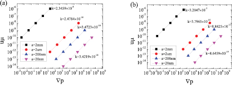
Figure 6. Permeability values for different particle sizes and models (a) for sc, (b) for hcp: the ordinate is the product of dynamic viscosity and apparent velocity, the abscissa is the opposite number of the pressure gradient, and the slope is the permeability.
Download figure:
Standard image High-resolution imageIn a previous study, Koponen et al [24] proposed a simple way of describing the capillary permeability with tortuosity,
where ε is porosity, c is the Kozeny coefficient that depends on the cross section of the capillaries, and τ is introduced to account for the complexity of the actual microscopic flow paths through the substance, which can be defined as the ratio of the (properly weighted) average length of the microscopic flow paths to the length of the system in the direction of the macroscopic flux [25]. S is the specific surface area of the holes, m−1. Generally, the specific surface area has inverse proportion to the size of an object. Considering equation (17), where k ~ 1/S2, k would be proportional to the square of the size of an object (hole or particle). In our simulation result, for both sc and hcp arrays, the ratios of the permeability of aggregates formed by 2 mm and 2 um particles are 2.35 × 10⁻⁸: 2.48 × 10⁻¹⁴ ≈ 1:10−6 and 3.20 × 10⁻⁹: 3.80 × 10⁻¹⁵ ≈ 1:10−6, respectively, in accordance with the proportional relation in equation (17). Due to the different wall boundary conditions, the permeability ratio of small to large particles does not meet the proportional relation. However, for the small particles where the slip boundary condition is applied, the proportional relation still exists, i.e. 3.47 × 10⁻¹⁶: 3.42 × 10⁻¹⁸ ≈ 1:10−2 and 8.84 × 10⁻¹⁷: 8.65 × 10⁻¹⁸ ≈ 1:10−2. Since the proportional relation of permeability and particle size has been found, we can use it for further study. This relation can be written as
where kx and k0 are the permeabilities of aggregates formed by particles with diameters ax and a0, respectively. k0, and a0 are known parameters. Therefore, for a given as ax, kx can be obtained. The relationship shown in equation (18) can dramatically simplify our model for sedimentation velocity. By combining the fluid dynamics property (equation (15)) and aggregate structure property (equation (18)), the direct relation of streaming velocity uf and seepage velocity us can be found,


Equations (19.1)–(19.4) are the relations between uf and us that correspond to the sc array of large particles, the sc array of small particles, the hcp array of large particles, and the hcp array of small particles, respectively. Equation (19) means that for an aggregate of spherical particles, the ratio of uf and us is a constant, having no relation to particle size. Note that other than several reasonable assumptions, there is no any empirical parameter introduced in equation (19).
From the velocities ratio of flowing around (uf) to seepage through (us) an aggregate, one can qualitatively discuss the effect of particle distribution in an aggregate on its sedimentation velocity. On the one hand, a compact distribution can lead to a small porosity (e.g. the porosity of the hcp array is only 0.2599, while the sc array is 0.4764), and small porosity would induce a large density of aggregates (shown in equation (9)). On the other hand, the particle distribution can dramatically affect the seepage velocity. For instance, the seepage velocity us of the hcp array is very small (less than 5% of uf), while that of the sc array is too large to ignore. Generally, for an aggregate with tiny permeability, the seepage velocity is negligible (such as the hcp array), therefore we may consider the aggregate as compact and non-penetrative.
Combining equations (9), (14), (15) and (19), the effects of the aggregate structure on the evolution and final concentration profiles were obtained. Figures 7 and 8 are for the sc and the hcp array, respectively. Figures 7(a) and (b) show the evolution of concentration profiles for the sc array aggregates. In this study, we applied aggregates with diameter aa = 50 nm (a) and 100 nm (b) to compare the effect of aggregate size on sedimentation velocity. Note that for a real suspension, the aggregate size is a distribution, which includes both very small and large aggregates. Relevant research indicates that aggregate size is positively correlated with the concentration of particles in a suspension [12–14]. In this sense, figures 7(a) and (b) can be considered as the evolutions of concentration profile in suspensions with lower and higher concentrations, respectively. On the one hand, for aggregate with smaller size, the final concentration profile is reached at t = 360 d, while for the larger size, it is reached at t = 90 d. This means that the concentration evolution of small aggregates is much slower than that of large aggregates. On the other hand, the sedimentation of large aggregates is more 'thorough' than small ones. This phenomenon can explain why suspensions with high concentration are more unstable than low concentrations.

Figure 7. Evolutions of concentration profiles for sc array aggregates where ρp/ρf = 2.5 and (a) aa = 50 nm, (b) aa = 100 nm with changing time, and final concentration distribution where aa = 50–200 nm and (c) ρp/ρf = 2, (d) ρp/ρf = 3. Insert: same data in a log–linear plot.
Download figure:
Standard image High-resolution image
Figure 8. Evolutions of concentration profiles for hcp array aggregates where ρp/ρf = 2.5 and (a) aa = 50 nm, (b) aa = 100 nm with changing time, and final concentration distribution where aa = 50–200 nm and (c) ρp/ρf = 2, (d) ρp/ρf = 3. Insert: same data in a log–linear plot.
Download figure:
Standard image High-resolution image
The final concentration profiles of the sc array aggregates with aa = 50–200 nm and relative density of primary particle ρp/ρf = 2 and 3 are shown in figures 7(c) and (d). Results indicate that, when the aggregate size aa > 100 nm, the final concentrations are near zero at relative position x/H > 0.1. From the log–linear plots, some detailed data can be acquired. Final concentration profiles dramatically rely on aggregate size. For instance, the relative concentration for aggregates aa = 50 nm in figure 7(c) is about 0.01 at x/H = 1, while for aa = 70 nm the relative concentration is close to 10−6. Similarly, the effect of density is also quite significant. With the increase of the density of primary particles, the degree of sedimentation significantly increases.
The evolutions of concentration profiles for the hcp array aggregates are shown in figures 8(a) and (b). To compare the difference between the sc and hcp arrays, the particle density and aggregate size are the same as that shown in figures 7(a) and (b). The evolution pattern of the hcp array is similar to the sc array, while there are also some differences. For instance, the dimensionless concentration c/c0 at t = 90 d and x/H = 0 is more than 6 in figure 8(a), but is larger than 4.5 for the sc array shown in figure 7(a). This result indicates the sedimentation of hcp array aggregates is faster than sc array ones. A similar result can also be found for 100 nm aggregates. From the log–linear plot in figure 8(b), it can be seen that at t = 30 d and x/H = 0.6, the dimensionless concentration c/c0 is 0.05, while c/c0 for the sc array is about 0.3, 5 times larger than the hcp array. As mentioned, the hcp array can lead to larger density and smaller seepage velocity. The former would increase the sedimentation velocity, and the latter may decrease it (see equations (13) and (14)). Based on these results, one can conclude that larger density can dramatically increase the sedimentation velocity even though the decrease in seepage velocity is against this tendency.
Figures 8(c) and (d), shows the final concentration profiles of hcp array aggregates with aa = 50–200 nm and relative density of primary particle ρp/ρf = 2 and 3. One can note that, with the increase of aggregate size, the concentration profile becomes more heterogeneous. For instance, the dimensionless concentrations c/c0 at x/H = 1 are about 0.01 and 0.02 for the hcp and sc array aggregates with diameter 50 nm and ρp/ρf = 2, respectively. While for aggregates with ρp/ρf = 3, the c/c0 at x/H = 1 are about 10−5 and 10−4. Thus, it can be concluded that the sedimentation of hcp array aggregates is more thorough than that of sc array aggregates.
It is worth noting that aggregates in suspensions always exhibit different sizes and shapes without having high compact structures. This has been defined as a fractal structure and is described by a fractal dimension [16]. Our model is expected to also be applicable to the aggregates of different sizes and structures if the aggregates are still and the permeability of aggregates was given at first. The limitation of the sphere-like shape for the aggregates is a result of the Stokes approximation. The permeability can be obtained by both numerical and experimental methods [21, 28]. Our model is therefore supposed to be suitable for solving the sedimentation problem of more complex suspension systems. In the present study, we chose sc and hcp structures because the permeability of the ordered structure is easier to obtain. Moreover, the porosities of the sc and hcp aggregates are 0.4764 and 0.2599, respectively. The large difference in porosities for sc and hcp aggregates can reflect in a clearer way the sensibility of our model.
4. Conclusion
The sedimentation of spherical particles in suspension was studied for the cases where aggregation of particles occurs or does not occur. Based on the gravity sedimentation and the concentration diffusion, the partial differential equation of concentration c(x,t) was deduced by the infinitesimal method. The finite volume method was employed to obtain the permeability of sc and hcp array aggregates. Based on the results, we successfully attained the ratios of streaming velocity uf and seepage velocity us for both sc and hcp aggregates formed by large or small particles. By investigating the evolution of the concentration profile and the final concentration profiles of particles and aggregates with different size and density, we found that an increment in both their size and density can dramatically increase the sedimentation velocity and degree. What is more, the sedimentation of hcp array aggregates is found to be faster and more thorough than sc array aggregates. Considering that the high concentration can increase the aggregate size, our result mathematically explains why suspensions with high particle concentration are more unstable.
Acknowledgments
The authors gratefully acknowledge the financial support of the National Natural Science Foundation of China (No. 51422604, 21276206) and the National 863 Program of China (No. 2013AA050402). This work was also supported by the China Fundamental Research Funds for the Central Universities. The authors would also like to thank Dr Jiafeng Geng for solving some equations.