

Abstract
Magnetization reversal of perpendicular anisotropy [Co/Au] multilayers patterned into micrometer wide stripes with a coercivity gradient along the stripes was investigated with polar magnetooptical Kerr effect microscopy. 1 mm-long stripes were bombarded with He+ ions of 10 keV energy to induce the gradient. It was shown that short pulses of a magnetic field applied perpendicularly to the sample plane move domain walls between up- and down-magnetized areas in a direction of regions with higher coercivities.
Export citation and abstract BibTeX RIS
1. Introduction
Composite Co based materials with perpendicular magnetic anisotropy (PMA) have an established use in mass data storage devices [1]. Multilayer (ML) films composed of transition ferromagnetic metals (TM) and noble-metal spacers, showing PMA, are intensively investigated because of potential applications in non-volatile random access memories [2]. Physical properties of TM-based ML PMA sytems, like saturation fields or their interlayer coupling, can be tailored [3] by adjusting thicknesses of the constituent layers. Alternatively post-deposition processes like bombardment by light ions [4–6], or annealing [7] may be used. For Au/Co/Au type MLs we have previously shown that a He+ ion bombardment can be used to precisely tailor the effective magnetic anisotropy of the Co layers [8] and that anisotropy gradients produced by continuously increasing/decreasing the ion fluence along one lateral direction can be employed to controllably move a domain wall (DW) by pulses of a homogenous magnetic field applied perpendicularly to the surface of the layers [9]. The possibility to control the DW position promises applications in transport of magnetic beads trapped by magnetostatic fields of DW [10, 11], in fluid mixing by moving particles [11], or in sensors registering maximum values of a field [12]. In homogenous films the position of DW can be changed by the field pulses, too. A significant advantage of layer systems with a lateral gradient of properties is that the direction of a DW propagation is determined by the gradient, that its position can be set, and that a thermally activated propagation is suppressed. All these layer systems need a propagation field that is lower than the field required for DW nucleation [9, 13]. Laterally graded anisotropy/coercivity systems provide an additional parameter to investigate the behavior of DWs in artificial structures [14]. From the practical point of view it is important to know whether the Co/Au systems for the controllable DW placement are scalable to micrometer widths, that are required for applications in lab-on-chip type devices involving magnetic beads [15–17]. In this paper we investigate the magnetization reversal, induced by the magnetic field pulses, in few-micrometer-wide patterned stripes having laterally graded PMA.
2. Experiment
Ti(4 nm)/Au(60 nm)/[Co(0.8 nm)/Au(1 nm)] multilayers, with N = 2 or 3, were deposited at room temperature on naturally oxidized Si(1 0 0) wafers by magnetron sputtering. The thickness of Co layers, sandwiched between Au, ensured PMA [3, 18, 19]. The strong ferromagnetic coupling between neighboring Co layers due to the thin Au spacer layers caused a simultaneous magnetization reversal of all Co layers in the layer system at a common switching field
  (see the discussion in section 2, and in [9]). Topographically elevated stripes of 995
  m length and widths w of 1
  m, 2
m, 2  m, 5
m, 5  m, 10
m, 10  m, and 20
  m, spaced about 100
  m apart, were produced by depositing the layer systems on a patterned lithography mask with subsequent lift-off (figure 1(d)). Patterning was carried out with electron beam lithography using a FEI Nova 6000 SEM microscope equipped with a Raith Elphy Plus system. We used a PMMA 950 resist of roughly 350 nm thickness and a 500
  C cm−2 electron dose at 30 keV energy. The samples were produced in batches of two; one with a continuous layer system used for the hysteresis investigation and the second, patterned one, for observation of the magnetic domains.
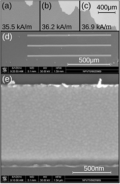
Figure 1. All images show the [Co(0.8 nm)/Au(1 nm)] structure. (a)–(c) P-MOKE images of the domain propagation, in sample that was not patterned, in perpendicularly applied magnetic field, (d) an electron microscopy image of 20
  m wide, and 995
  m long stripes, (e) a close-up image of a 1
  m wide stripe showing the grainy structure of the MLs.
Download figure:
Standard image High-resolution imageTo create the lateral gradient of the magnetic anisotropy the stripes were subject to light-ion bombardment (10 keV He+ ions) with a fluence varying linearly along the longer edges of the stripes from roughly zero (the ion beam extended beyond the  mm2 aperture—see figure 1 in [9]) to approximately 1015 ions cm−2. We made the gradient by placing an edge of the beam at one end of the stripe, so that its whole length was exposed to the ions (the placement precision was about 0.1 mm), and then moving the edge to the other end of the stripe with a constant velocity. In practice several stripes were bombarded at a time.
The samples were investigated with a magnetooptical Kerr effect magnetometer in polar configuration (P-MOKE); the sweep rate was 0.6 (kA m−1) s−1, and the laser spot diameter was about 0.5 mm. The magnetic domain structure of the stripes, and of the continuous layer systems was observed by a magnetooptical Kerr microscope. The following procedure to obtain each image of the domains was used: The samples were first saturated by applying a magnetic field of 80 kA m−1 which was oriented perpendicularly to the plane of the substrates. Then the field was switched off and a greyscale image  (x, y) of the sample with 16 bit greyscale depth, resulting from the averaging over 20 frames, was recorded (Hamamatsu ORCA-05G digital camera,
  pixels,
 m field of view, and a total image acquisition time of approx. 3 s). We applied then a given field, H, of an opposite direction to the previously used and after switching the field off we recorded a second image
  (x, y). An arithmetic difference between these two images
  –
– (x, y) gave us the information about the domains present in the sample [20]. Areas in which magnetic moments reversed their orientation were either brighter or darker than the rest within the difference image (figure 2). For the stripes of 2
  m width we recorded the images slightly out-of-focus because otherwise a mechanical displacement in our system, and 'artificial' dark edges produced by it (see for example the bottom domain in figure 5(a)), made the determination of domain wall positions impossible. We were not able to observe the domains in 1
  m wide stripes.

Figure 2. Sketch of the magnetic configuration of the sample. At first, the sample is saturated with all magnetic moments pointing upwards. (Note that the Co layers in the MLs are strongly coupled so that magnetic moments point approximately in the same direction through the whole film thickness.) After the application of magnetic field of opposite direction some of the moments, those in the areas bombarded with higher fluence, reverse (bright arrows). The difference between the image brightnesses, after and before the change, in the regions where the moments reversed is high—these areas are bright (or dark, depending on which image is a minuend) in the difference MOKE images (compare figure 3).
Download figure:
Standard image High-resolution imageDue to the differences between imaging of the stripes with w = 2  m and the wider ones we used two different procedures to estimate the DW position (or length of the domain):
- (a)For the stripes with
 5 m, using the ImageJ [21] program, we obtained brightness data from the arithmetic difference image (x, y) (figure 3(a)). Then the image was thresholded [22] (figure 3(b)). The resulting binary image was divided into rectangles, with sides parallel to the image edges, so that each such rectangle contained one bright area which we identified with a single domain (figure 3(b)). A linear regression over the individual (x, y) positions of centers of all white pixels within a given rectangle was performed to determine the orientation of the long axis of the domain with respect to the x-axis of the image (see figure 3(c)). Subsequently we binned the pixels within the rectangle with respect to their distance to the regression line (with bin size equal to pixel width, approx. 0.7 m). An exemplary set of pixels belonging to one bin is displayed in figure 3(c) in grey color. Then the number (bin = 1,2,3,...) of bright pixels within each bin (corresponding to a line with defined distance to the regression line) was determined. Averaging over these numbers resulted in . For all bins that contain more than 0.9 pixels we calculated the length L of the bin along the regression line (figure 3(c)). The average over the different Ls (for the different bins) is a measure of the domain length which we use in this paper.
 - (b)For the 2m stripes we manually placed an overlay [21] (a mask of 10 pixels width and length of the stripe within the image, i.e. over 1100 pixels) on the area of the image corresponding to a given stripe. For each measurement with different magnetic field pulse an image intensity profile [] was determined along the long stripe/mask axis by averaging the values over the 10 pixel widths (, where is a pixel count along the width of the area at position x). Due to the still weak contrast in the profile between the areas corresponding to the two magnetization states we averaged the profile with a simple (i.e. not weighted) moving average (of 60 points). The domain wall position was then determined as the pixel position along the averaged profile where the brightness value becomes less than the brightness = . The standard deviation of positions obtained that way, determined from ten consecutive measurements of a single image of an exemplary domain, was 4.5 m. Note that for the 2 m stripes we do not determine the lengths of domains but only the position of the DWs to avoid additional error associated with finding the position of the opposite end of the domain (see figure 7).


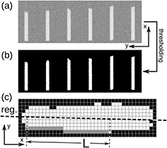
Figure 3. (a) Exemplary difference image  (x, y) (see section 2) of 20
  m wide domains (the same as in figure 5(b) but rotated by 90 degrees), (b) the corresponding binary image obtained with thresholding of
  (x, y). (c) White and grey pixels schematically show one domain (see the description in section 2). Grey squares indicate pixels belonging to one bin. In this example their distance to the regression line (thick dashed line) is more than 3 and less than 4 times the pixel width. L denotes the length of the bin, along the regression line, determined from the orthogonal projection on that line.
Download figure:
Standard image High-resolution imageAll the measurements were performed at room temperature.
3. Discussion
M(H) hysteresis loops of the continuous layer samples have saturation field values close to 40 kA m−1 and their coercivities HC range from 33 to 40 kA m−1 (figure 4). Whereas for N = 2 the hysteresis loop is square and therefore HC is about equal to HS, the saturation is approached more gradually for the N = 3 samples. The gradual approach may be a result of roughness that increases with the total thickness of the film. The roughness in turn produces a magnetostatic contribution [23] that causes an increase of HS [24]. The coercivity of ML with N = 3 is slightly lower than for N = 2. In Co/Au systems the PMA is due primarily to surface contribution which, for  nm, is about
  Jm−3 [25], that is more than twice the effective magnetocrystalline anisotropy contribution (
 Jm−3). We attribute thus the difference in HC to the influence of interface roughness [8]. Hysteresis loops measured for patterned films, i.e. for the stripes (figure 4(b)), show higher coercivities. We think that there are two reasons for this. First, with decreasing the area of the magnetic film by the patterning (a substrate coverage for 2
  m stripes is approx. 2%) the number of nucleation centers decreases, too. Second, the patterning can introduce new pinning centers which delay nucleation. In the quasistatic regime of measurement that we used the magnetization of all Co layers reverses simultaneously. The dynamics of DW motion, however, may be slightly different in each Co layer. Nevertheless, after the removal of the driving field the DWs in neighboring layers relax to each other [20]. We do not observe, as expected [26], stripe domains for small number of repetitions (
 ) of Co layers. The magnetization reversal in the continuous layer takes place by domain propagation, from sparsely placed nucleation centers (figures 1(a)–(c)), in a relatively narrow field range. Because we used short field pulses we were not analyzing the thermal activation of reversal [27, 28] that has decay constants of several seconds if the field is less than the quasi-static value of HC [29].
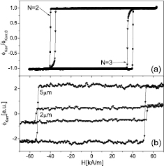
Figure 4. (a) Characteristic P-MOKE hysteresis loops of continuous [Co(0.8 nm)/Au(1 nm)] MLs. (b) The analogous loops for the [Co(0.8 nm)/Au(1 nm)]
 layer patterned into 5 and 2
  m wide stripes.
Download figure:
Standard image High-resolution imageThe morphology of our patterned samples is shown in figures 1(d) and (e). One can see that the stripes are grainy, with in-plane grain sizes in the 50–100 nm range. The grains are larger than in similar evaporated MLs [29], which, however, had a thinner buffer. The columnar structure of the thick Au buffer is responsible for that. We note that a DW width in our Co/Au MLs [26] is close to the grain sizes and the grains may act as pinning centers [27]. The bright spots along the upper edge of the 1  m stripe are remnants of 'rabbit ears' [30] which may result in some additional DW pinning, too (see discussion of figure 5).
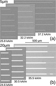
Figure 5. Representative, recorded in zero field (see section 2), MOKE images of the domains in the 5 and 20  m wide stripes, of [Co(0.8 nm)/Au(1 nm)]
 MLs (N = 2 for 20
  m stripes, and N = 3 for 5
  m stripes), with the effective anisotropy/coercivity gradient along their lengths, for different values of the perpendicularly applied magnetic field pulses.
Download figure:
Standard image High-resolution imageRepresentative images of the zero field domain configuration (see section 2), as a function of the strength of the applied field pulses, are shown in figure 5 (note that all stripes in the images were bombarded). The domains nucleated first at the ends of the stripes bombarded by the highest ion fluence (left hand side of the stripes of figure 1(d)). As already shown [8], the bombardment of Au/Co MLs leads to a decrease of the effective PMA, mainly through the lowering of the interface contribution probably due to an increased roughness of interfaces. The lowered anisotropy decreases the energy barrier required for the reversal of magnetic moments [19] and the reversal, although random in nature, starts usually there. The domains begin to appear at  (
( of the continuous ML) which is much more than one would expect knowing that 1015 ions cm−2 fluence reduces
  of 0.6 nm thick Co layers by almost 100% [31]. We attribute this 'delayed' nucleation to a low density of nucleation centers in our MLs, even in the patterned ones. We should note, that in the stripes that were not bombarded there was no visible preference for the nucleation of the domains in any specific area and that the complete reversal took place within approx. 4 kA m−1 field range, while in the bombarded samples the field range of reversal was about 15 kA m−1 (figure 7). With increasing H the domains gradually grew to the right, in the direction opposite to the fluence gradient, as we already demonstrated for the case of centimeter-sized samples [9].
We often observed that a separate domain nucleated to the right of the domain expanding from the left (LD) (see the lowest stripe in figure 5(b) for H = 35.5 kA m−1). This is a consequence of the fact that the right ends of the stripes (not visible in the images) were bombarded with almost zero fluence and the HC is there almost the same as in the as-deposited sample [8]. The domains could therefore nucleate far from the reversal front of the LD and within the approx. 1 s duration of the field pulse did not have enough time to expand to the left to merge with the LD. Such a scenario is more probable in wider stripes that contain more nucleation centers. Four of the six domains shown in figure 5(b) for H = 35.5 kA m−1 have almost the same length. Note, however, that the right end of the longest domain has approx. the same position as the right end of the small domain located in front of the large domain in the lowest stripe of the image. It is thus very likely that the situation observed in the lowest stripe is an intermediate state between what is seen in the other four stripes and in the one with the longest domain. In the widest stripes (w = 20  m) we observed (figure 5(b) for H = 24.6 kA m−1) that the DWs were not always perpendicular to their longer edges. This would be energetically favorable in homogenous layers because a longer DW necessitates more DW energy [32]. Therefore they were probably pinned on some edge defects, like the 'rabbit ears' (figure 1(e)) which may act as sources of pinning fields similar to gate magnets in [33]. The grain boundaries (figure 1(e)), on the other hand, create a random pinning field which determines dynamic properties of the DWs [34] that are not investigated here. The DWs can pin on geometrical defects, like in the case of a constriction in the lowest stripe of figure 5(a) for H = 37.2 kA m−1 (see dependence for first domain in figure 7(b)).
Some features of the DWs behavior seen in figure 5 can be explained by simple phenomenological considerations. As the dependence of Hc, which is an approximate measure for the nucleation field Hn, on the ion fluence can be approximated by an exponential function (figure 3 in [31]) and the fluence as a function of distance from one end of the 1 mm-long stripe (see section 2) is linear we can approximate:  , where x is the position along the stripe. This can be used to estimate the field dependence of the barrier height to nucleation,
  , in the external field H [27]:

where En is the nucleation energy; typically the exponent is taken between 1 and 2 [27]. The magnetization reversal can be activated thermally [27, 28] and its rate, r, or frequency may be described by an Arrhenius type law:
where r0 is some constant, and T is the temperature. The absolute value of r0 is not important for the present estimate, as in the model only relative values give the important information. Inserting (1) into (2) and multiplying this by the time interval  for which the field was applied we obtained an expression proportional to a nucleation probability as a function of the lateral coordinate x and the temperature. In the model we divided the stripe along its length into 1000 parts, and calculated for each of them its nucleation probability P(x) with a constant value of the product of time interval
  and base frequency r0 of 1. We assumed additionally that within the duration of the field pulse each nucleated domain grew by 20
  m in positive and negative x-direction (this extension roughly corresponds to the minimum size of the imaged domains that nucleate to the right of LD). Exemplary results of this qualitative model are shown in figure 6. For each of 1000 parts of the stripe, and for each value of H, a pseudorandom number within the range between 0 and 1 was generated. If this number was less than P(x) of this part of the stripe the domain nucleated there. Similar to the images shown in figure 5 the domains grow with increasing H. For some values of H domains nucleate to the right of the reversal front and in some cases the length of the domain is less for higher H (two bottom domains), as is often observed experimentally (figure 7).

Figure 6. Exemplary simulated magnetic configuration obtained from the phenomenological model described in section 3. The field pulse strength increases from the top to bottom stripe (H = 0.01, 0.05, 0.10, 0.15, 0.2, 0.25, 0.3 [a.u.]). The parameters used in the model are: H0 = 1, En = 1, r0 = 1,  , and T = 0.1.
Download figure:
Standard image High-resolution image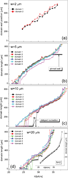
Figure 7. (a) The positions of the moving ends of the domains in the 2  m-wide stripe of [Co(0.8 nm)/Au(1 nm)]
 ML obtained from MOKE images, recorded in zero field (see section 2), as a function of the strength of the perpendicularly applied magnetic field pulses. (b)–(d) Similar dependencies for other widths of the stripes. In the inset of panel (d) the dependencies for N = 2 are also shown. Note that the line protruding to the right in panel (b) corresponds to the DW that was pinned on the defect—the lowest domain seen in figure 5(a) for H = 37.2 kA m−1.
Download figure:
Standard image High-resolution image
The nucleation processes are random in a sense that we cannot predict an exact domain configuration for a given H. The overall trend, however, is clearly visible in figure 7. With increasing H the domains grew in length l for the stripes of all widths in one direction, which is consistent with the gradient of the ion fluence. Depending on the number of nucleation centers the l(H) curve is similar for each stripe of the sample (figures 7(a) and (b)) or differs much if the nucleation center density is low (figure 7(c)). In one stripe a domain nucleated when H exceeded 28 kA m−1 while in other stripes a field of 22.5 kA m−1 was enough to initiate the nucleation. The reproducibility of the DW positions was relatively good: for six 10  m-wide stripes the average standard deviation of their length, for ten consecutive pulses of H = 35 kA m−1, was 10
  m. In the narrower stripes (
 m) the domains appear roughly simultaneously, which may be caused by nucleation at their bombarded ends [35] and not as in wider stripes at random sites within the larger area. When H increases towards the intrinsic Hc the reversed domains expand to the whole stripe. The overall character of magnetization reversal in MLs with N = 2 is similar although the domains in the particular case shown in figure 7 nucleate at lower H.
4. Conclusions
We have investigated domain nucleation and propagation in micrometer-wide stripes of the perpendicular magnetic anisotropy [Co/Au] multilayers with an anisotropy gradient along one lateral coordinate, created by 10 keV He+ ion bombardment with increasing dose along this coordinate. The magnetization reversal was induced by short, one second long, pulses of magnetic field that was perpendicular to the sample plane. The magnetization reversal was observed in remanence by magnetooptical Kerr microscopy. Edge defects introduced by the patterning did not change the character of the reversal as compared to the extended samples that we investigated previously. We showed that the position of the domain walls can be set by the applied field strength with relatively high reproducibility which proves their potential for applications.
Acknowledgment
The work was financed by the National Science Centre Poland under HARMONIA funding scheme for international research projects decision No. DEC-2013/08/M/ST3/00960 and by the German Academic Exchange Service (DAAD).