


ABSTRACT
We study the buoyant rise of magnetic flux tubes embedded in an adiabatic stratification using two-and three-dimensional, magnetohydrodynamic simulations. We analyze the dependence of the tube evolution on the field line twist and on the curvature of the tube axis in different diffusion regimes. To be able to achieve a comparatively high spatial resolution we use the FLASH code, which has a built-in Adaptive Mesh Refinement (AMR) capability. Our 3D experiments reach Reynolds numbers that permit a reasonable comparison of the results with those of previous 2D simulations. When the experiments are run without AMR, hence with a comparatively large diffusivity, the amount of longitudinal magnetic flux retained inside the tube increases with the curvature of the tube axis. However, when a low-diffusion regime is reached by using the AMR algorithms, the magnetic twist is able to prevent the splitting of the magnetic loop into vortex tubes and the loop curvature does not play any significant role. We detect the generation of vorticity in the main body of the tube of opposite sign on the opposite sides of the apex. This is a consequence of the inhomogeneity of the azimuthal component of the field on the flux surfaces. The lift force associated with this global vorticity makes the flanks of the tube move away from their initial vertical plane in an antisymmetric fashion. The trajectories have an oscillatory motion superimposed, due to the shedding of vortex rolls to the wake, which creates a Von Karman street.
Export citation and abstract BibTeX RIS
1. INTRODUCTION
Starting with the seminal paper of Parker (1977), a large body of work along the past four decades has shed light on the key magnetohydrodynamic (MHD) processes that affect the rise of magnetic flux tubes across a stratified medium like the solar convection zone. An approach, not followed in this paper, is to study the large-scale flux tube evolution by way of simple one-dimensional models using the thin magnetic flux tube approximation (Roberts & Webb 1978; Spruit 1981): such models allowed the study of the large-scale motion of flux tubes from the bottom of the convection zone to the near-surface layers (e.g., Moreno-Insertis 1986; D'Silva & Choudhuri 1993; Fan et al. 1993, 1994; Caligari et al. 1995; Weber et al. 2011), including a detailed stratification of the solar interior. In those papers, the moving magnetic tube and the stratified background are assumed to be distinct media, with the latter influencing, but being unperturbed by, the former. The thin flux tube approximation assumes the radius of the flux tube to be much smaller than the other relevant length-scales in the problem (including pressure scale height and radius of curvature of the tube) and does not allow for the study of how the tube cross-section evolves. A new class of models that study the 3D evolution of magnetic tube-like concentrations rising through the depth range of the convection zone has appeared in recent years (Fan 2008; Jouve & Brun 2009; Jouve et al. 2013; Pinto & Brun 2013): in those papers, the anelastic three-dimensional fluid-dynamics equations are solved for a spherical shell with the stratification of the solar convection zone. The last three of those models include self-consistent large-scale convective motions that encompass the whole range of depths of the simulated domain. Those calculations are computationally demanding so they cannot reach high viscous and magnetic Reynolds numbers. On the other hand, it is interesting to note that, in what concerns the motion of the tube-like domains, they recover many of the basic results obtained with the older thin-tube models.
A different approach followed in the past decades, and also in the present paper, is to study the internal dynamics of buoyant magnetic tube-like regions by using two- or three-dimensional models with a simplified, adiabatic and cartesian background stratification. The simulations of Schüssler (1979), Longcope et al. (1996), Moreno-Insertis & Emonet (1996), Emonet & Moreno-Insertis (1998), Fan et al. (1998), Hughes & Falle (1998), Emonet et al. (2001) and Cheung et al. (2006) among others, in 2D, and Dorch & Nordlund (1998), Dorch et al. (1999), Fan et al. (1999) and Abbett et al. (2000), in 3D, examined, in particular, the physical mechanisms whereby the moving magnetic flux tubes can maintain (or otherwise lose) their coherence during the rise. Schüssler (1979) showed that an untwisted, rising horizontal tube splits into counter-rotating vortices after rising a height comparable to the initial tube diameter. Longcope et al. (1996) carried out a similar experiment with higher spatial resolution; they explained the sideways motion of the counter-rotating vortex tubes through the combined action of the buoyancy and lift forces exerted by the surrounding flow. Moreno-Insertis & Emonet (1996) and Emonet & Moreno-Insertis (1998) demonstrated that a sufficient amount of twist of the magnetic field lines can provide the magnetic tension necessary to prevent the splitting of the tube. They obtained a criterion, namely,  with R the tube radius, Hp the pressure scale-height, and Ψ the pitch angle of the field lines in the dynamically relevant part of the tube, for the splitting into sideways expanding vortices to be substantially reduced, with the tube thus retaining a good fraction of its original magnetic flux. Additionally, Emonet & Moreno-Insertis (1998) explained the importance of the magnetic boundary layer at the periphery of the tube as a site of vorticity generation: vorticity-loaded fluid elements sliding along the boundary layer are carried to the wake where they accumulate. This is a process reminiscent of the behavior of flows around rising air bubbles in liquids or past rigid cylindrical rods (e.g., Davies & Taylor 1950; Collins 1965; Parlange 1969; Berger & Wille 1972; Wegener & Parlange 1973; Hnat & Buckmaster 1976; Ryskin & Leal 1984; Christov & Volkov 1985; Williamson 1988a, 1988b, 1996; Norberg 1994; Rast 1998).
The phenomenon of vortex shedding from the wake was analyzed by Fan et al. (1998) and Emonet et al. (2001): the vortex rolls can be ejected alternatively from each side of the main tube creating a trailing Von Kármán vortex street: each emission of a vortex roll leaves the head with an excess vorticity of the same amount and opposite sign. The alternation in the sign of the vorticity of the head entails an oscillating lift force which, when combined with the drag and buoyancy forces, leads in the simplest cases to an oscillatory sideways motion of the tube's head superimposed on its rise. As shown by Emonet et al. (2001), in more complicated situations, when the amount of vorticity in the wake is large, vortex shedding leads to large lift forces in the tube head; when the lift force is dominant, the complication of the trajectory of the tube head can be considerable (see, e.g., their Figure 6). This is probably the reason for the peculiar trajectory resulting from the simulation by Hughes & Falle (1998), who used an adaptive-grid numerical code that allowed them to reach high Reynolds numbers.
The importance of reaching high Reynolds numbers in this kind of experiment was clearly demonstrated in the 2D simulations by Cheung et al. (2006). These authors used the FLASH code (Fryxell et al. 2000), and applied the code's Adaptive Mesh Refinement (AMR) feature to study in detail the dependence of the results on the effective Reynolds number of the flows; the latter was determined by finding the ratio of the actual thickness of the boundary layer measured in the experiment to the tube diameter. When the magnetic Reynolds number (Rem) reaches values around several hundred, the smooth vorticity profile of the wake characteristic of lower-Rem experiments turns into a complicated distribution with a hierarchy of vortices down to very small sizes. Importantly, they also showed that the fraction of magnetic flux retained inside the tube greatly increases when Rem grows from below 100 up to a few hundred; the increase seems to level off when Rem enters the range around a few thousand. In addition, the authors confirmed previous results in that the amount of flux retained in the tube's head decreases with decreasing levels of field line twist around the axis even in the high-resolution, high-Rem regime. They also reproduced the vortex-shedding phenomenon observed in lower-Rem calculations.
There are also a few instances of three-dimensional simulations that study the coherence of magnetic tubes rising in idealized stratifications. Dorch & Nordlund (1998) studied the effect of the transverse component of the magnetic field on the tube's evolution: their tubes with a purely axial (i.e., untwisted) field suffered the splitting into vortex tubes also obtained by the authors reported above. In a few of their experiments, however, they introduced a transverse magnetic field superimposed on the axial component: the transverse field was a mixture of a simple twisted structure (obtained via the curl of a Gaussian-shaped vector potential) and a random component. The resulting strength of the transverse component was high enough for the rising tube to maintain its coherence. In the corresponding figure in their paper one can even see the formation of a vortex street in the wake, but the authors do not mention this fact. Dorch et al. (1999) carried out another 3D experiment, this time simulating the rise of an Ω-loop, and obtained that the apex of the tube behaves as in the simple case of a 2D twisted tube. Abbett et al. (2000), finally, carried out 3D simulations of rising Ω-loops also using the anelastic approximation. Their results concur with those of the 2D simulations of Moreno-Insertis & Emonet (1996) and Emonet & Moreno-Insertis (1998) for tubes with an amount of twist at or above the critical limit obtained by those authors. For subcritical twist, however, Abbett et al. (2000) showed that the fragmentation of the Ω-loop depends on the loop's curvature; the higher the curvature, the smaller the magnetic flux loss from the main body of the rising tube. All these early 3D simulations, however, necessarily had a comparatively reduced number of grid points. Their Reynolds number, therefore, was most likely not very high.
Our aim in the present paper is to study the physics of the rise of a buoyant magnetic flux tube through an adiabatically stratified medium in three spatial dimensions with high spatial resolution of the tube and its boundary layers, thus reaching comparatively high values of the Reynolds number. We try to study in some detail the general features of the rise and also address the question of the fragmentation of the tube and of the amount of magnetic flux retained in its main body when 3D and comparatively high Reynolds number are used. In order to diminish the numerical diffusivity, we performed the simulations using the FLASH code (Fryxell et al. 2000) with its AMR feature. The governing system of equations, the numerical methods and the simulation setup are detailed in Section 2. The global properties of the flux tube evolution are described in Section 3. In Section 4, we study the dependence of the tube fragmentation on the curvature (Sections 4.1) and on the amount of twist (Sections 4.2) for different levels of spatial resolution, or, more precisely, of mesh refinement of the highly structured subdomains. In addition, Section 4.3 describes the differences in the structure and dynamics of the Ω-loop apex for the various simulations. In Section 5, we analyze the global effects of the aerodynamic lift force on the legs of the Ω-loops. Finally, Section 6 contains a discussion and conclusions.
2. SETUP OF THE SIMULATIONS
We carry out a series of simulations for a simple compressible and electrically conducting medium. As equation of state we choose the ideal gas law ( ), with ρ, p and T the mass density, gas pressure, and temperature respectively,
  the universal gas constant and μ the atomic mass per particle. For a fully ionized hydrogen plasma with realistic mass ratios, μ = 0.5. Since we are not concerned with the thermodynamics of the problem, the temperature scale is not important and we use μ = 1. The system is governed by the compressible ideal MHD equations. In conservation form and using MKS units, they are


where ⨂ denotes the tensor product and  ,
,  ,
,  stand for the velocity field, magnetic field and gravitational acceleration, respectively. Cartesian coordinates (x, y, z) are adopted, with z being height, i.e.,
  with g > 0. pT is the total (magnetic + gas) pressure and e is the specific total energy, i.e., the sum of the kinetic and internal energies per unit mass and B2/(2μ0 ρ).
2.1. Numerical Method
The simulations were carried out using the FLASH 2.5 code (Fryxell et al. 2000). This code implements a Riemann solver that is formally second-order accurate in time and space. The advective terms are discretized using a slope limited Total Variation Diminishing (TVD) scheme and the time-stepping is performed using an explicit Hancock-type scheme.
Effects associated with thermal, viscous or ohmic transport phenomena have not been explicitly taken into account in the MHD Equations (1)–(4). Yet, artificial diffusive effects are always present in all simulations as a result of the diffusion inherent in the numerical scheme. In our case numerical diffusion is due to the TVD scheme acting to limit gradients at the level of the numerical grid spacing. In astrophysical problems, the most general situation is to have very large physical viscous and magnetic Reynolds numbers, the solar interior being but one example thereof. To get as close as possible to the astrophysical values in the numerical simulation, one has to diminish the numerical diffusive effects, which requires increasing the spatial resolution of the grid, thus yielding higher effective Reynolds numbers. To that end, we use the AMR capability of FLASH to increase the grid resolution in regions where it is required. Briefly, using AMR, the cartesian domain is divided into adjacent square or cube blocks, each block consisting, by default in the code, of 8 × 8 (2D) or 8 × 8 × 8 (3D) grid cells. All the blocks are checked to determine if they should be redefined within a time interval which must be much smaller than the time that the tube needs to cross one block, i.e., we set to check it every ten timesteps. If the normalized second-order spatial derivative of the absolute field strength exceeds some fixed threshold in any grid cell, the resolution of the corresponding block is doubled using second-order interpolation. Then, the original block is split into four (2D) or eight sub-blocks (3D), increasing the refinement level by one. The reverse process happens when the second order spatial derivative of the absolute field strength is smaller than some threshold for all four (2D) or eight (3D) sub-blocks.
For further details on the FLASH code and its AMR algorithm, the reader is referred to Fryxell et al. (2000) and the PARAMESH website http://www.physics.drexel.edu/~olson/paramesh-doc/Users_manual/amr.html
2.2. Initial and Boundary Conditions
The initial plane-parallel background is an adiabatically stratified polytrope described by the following density, pressure and temperature profiles:


where

ρo, po and To are constant values, zo is a reference height, and n is the polytropic index. The entropy profile for the stratification given through (5)–(7) fulfills the following relation:

with γ the specific heat ratio (chosen here γ = 5/3) and cV the constant specific heat. To prevent the development of convective cells in the experiment we choose an isentropic stratification, i.e., we set n = γ/(γ−1) = 2.5 so that the right-hand side of Equation (8) vanishes.  is the pressure scale-height at z = zo, as follows immediately from Equations (5) and 7. We use
  , ρo, po, and To as units of length, density, pressure, and temperature, respectively. For the velocity, we choose as unit the isothermal sound speed at zo, namely,
  As magnetic field unit we choose
  The non-dimensional units allow to apply these simulations in various problems where the stratification of the atmosphere is close enough to adiabatic. In the Sun, this problem could be implemented everywhere in the convection zone as long as it is not too close to the photosphere. By way of example, for the conversion of variables one could use the following set of values for the units, which are adequate to the deep convection zone:
  km, To = 2.2 106 K, po = 6.5 1013 erg cm−3, ρo = 0.22 g cm−3.
Our aim is to have an initial distribution of magnetic field, pressure and density that leads to the development of a rising Ω-loop. To that end, we follow in the steps of Fan (2001), and Archontis et al. (2004), and many later references that use similar distributions. The initial magnetic flux tube is taken to be axisymmetric with the axis lying along the y-axis at a height z = zo. In cylindrical coordinates (r, ϕ, y) centered on the tube axis, the longitudinal  and azimuthal
  components of the magnetic field have the following form:


where R provides a measure for the radius of the flux tube and Bc is the initial magnetic strength along the tube axis. This prescription leads to twisted magnetic field lines that lie on the cylindrical surfaces r = const. For all simulations in this paper, R = 0.12 and Bc = 0.2, corresponding to a local plasma β = 50. The magnetic field is set to zero beyond r = 2R. At this radius the exponentials in Equations (9) and (10) are already below 0.02; the small resulting tangential discontinuity for the field is dynamically unimportant. λ in Equation (10) is the dimensionless twist parameter. The pitch of the twisted field lines is given by  independently of r. As part of our parameter study, simulations with different values of λ were carried out.
The magnetic field distribution given by Equations (9) and (10) leads to a Lorentz force pointing inward the radial direction. One can easily compensate for it by correcting for the gas pressure, as follows:
with

so, after applying this correction, there is still force equilibrium. Now, in the 3D simulations, we are interested in studying the rise of Ω-loops. To induce their development, we then introduce a density perturbation localized around y = y0 with spatial extent χ:

and add it to the background stratification:

maintaining the pressure as given in Equation (11). Note that the entropy throughout the computational domain is kept unchanged, which is different to Fan (2001) and Archontis et al. (2004). Yet, the results published in this paper are not dependent on the exact nature of this perturbation, whether isentropic or isothermal. For a discussion of these perturbations see Moreno-Insertis (1983). From Equation (12) we see that the tube is neutrally buoyant ( ) for
) for  so at time t = 0 it is in complete force equilibrium there. On the other hand, the perturbation (12) leads to a density deficit of order
  around y = y0, which is adequate to start the dynamical evolution of the tube (see Moreno-Insertis 1983). From the Gaussian shape of the density deficit (Equation (12)), we can estimate the radius of curvature of the resulting Ω-loop as follows: in this paper we are going to pursue the loops until their apex has risen across a distance of a few pressure scale-heights
  . Hence, we expect the radius of curvature of the rising loop to be of order

at its apex. Consequently, we will use χ as the parameter controlling the radius of curvature in the rising loops. When  the initial condition leads to an uniformly buoyant tube that rises maintaining a horizontal shape.
Concerning the simulation domain, the size of the 3D box was either 2.6 × 10.4 × 2.6 or, for some experiments, 2.6 × 15.7 × 2.6. The value 2.6 in the transverse directions x and z provides enough room to accommodate a thin flux tube (R = 0.12) inside it, even after it expands along the rise. In the y direction, we need room to fully include the developing Ω-loop, whose expected radius of curvature is as given in Equation (14). Hence the elongated shape of the box along y and also the larger y-size for the 3D simulations with the highest χ. In the 2D experiments, the box was 2.6 × 2.6 in all cases. The center of the initial tube was always located at z = zo = 11.1, but the distance of that point to the top and bottom lids of the box was varied slightly to accommodate for the needs of each simulation (like the distance descended by the lower segments of the tube). The experiments are finished when the top layers of the tube reached z ≥ 12.3. The pressure contrast between those two levels (z = 11.1 and z = 12.3) is 5.2, which corresponds to 1.6 pressure scale-heights. The density contrast is 2.7.
Table 1 summarizes the different experiments carried out for this paper. The main parameters we vary, following the explanations just given, are χ, i.e., the parameter associated with the radius of curvature (4th column in the table), the twist parameter λ (5th column), and the number of levels of refinement allowed in the AMR algorithm over the basic, non-refined grid (6th column). We label the experiments (first column) using those parameters. For example,  is a simulation with χ = 1.5, λ = 1/8 and (H ) the highest number of refinement levels (in fact, AMR = 2) over the basic grid. Other experiments have a single level of refinement (AMR = 1, indicated with an "M") or no refinement (AMR = 0, indicated with an "L").
  is the tag used for the case when
  in Equation (12); this corresponds to uniform buoyancy along the y-axis which leads to a horizontal rising tube, i.e., a 2D experiment. Further columns in the table contain the box size (2nd column), the number of grid points if the whole box were covered by a grid at the highest level of AMR resolution in that experiment (3rd column) and, by way of results, the amount of flux retained in the tube toward the end of the calculated evolution (9th column) and the effective diameter of the head of the tube at time t ∼ 50 (10th column). The table also contains a representative value of the Reynolds number of each experiment (7th column) which we see varies as a function of the initial parameters, in particular of the number of AMR levels. Given that the viscosity in the model is numerical (the equations solved do not explicitly include a viscous term), one cannot directly compute the Reynolds number from characteristic lengths and flow speeds. We use the procedure described in
Table 1. List of the Simulations Described in the Paper
| Name | Box Size | Grid Points | χ | λ | AMR | Re | ν |
 (%) (%) |
Dhead |
|---|---|---|---|---|---|---|---|---|---|

|
2.6, 2.6 | 512, 512 |

|
0 | 2 | ⋯ | ⋯ | 8 | 0.20 |

|
2.6, 2.6 | 512, 512 |

|
1/16 | 2 | 190 | 3 10−4 | 20 | 0.40 |

|
2.6, 2.6 | 128, 128 |

|
1/8 | 0 | 3.5 | 10−2 | 5 | 0.36 |

|
2.6, 2.6 | 512, 512 |

|
1/8 | 2 | 190 | 3 10−4 | 47 | 0.68 |

|
2.6, 2.6 | 512, 512 |

|
1/4 | 2 | 190 | 4 10−4 | 72 | 0.74 |

|
2.6, 15.7, 2.6 | 512, 3072, 512 | 2.1 | 1/16 | 2 | 290 | 10−4 | 32 | 0.42 |

|
2.6, 15.7, 2.6 | 128, 768, 128 | 2.1 | 1/8 | 0 | 7.5 | 6 10−3 | 20 | 0.46 |

|
2.6, 15.7, 2.6 | 256, 1536, 256 | 2.1 | 1/8 | 1 | 100 | 10−3 | 41 | 0.60 |

|
2.6, 15.7, 2.6 | 512, 3072, 512 | 2.1 | 1/8 | 2 | 290 | 2 10−4 | 48 | 0.54 |

|
2.6, 15.7, 2.6 | 512, 3072, 512 | 2.1 | 1/4 | 2 | 290 | 3 10−4 | 72 | 0.74 |

|
2.6, 10.4, 2.6 | 128, 512, 128 | 1.5 | 0 | 0 | ⋯ | ⋯ | 16 | 0.26 |

|
2.6, 10.4, 2.6 | 512, 2048, 512 | 1.5 | 0 | 2 | ⋯ | ⋯ | 18 | 0.18 |

|
2.6, 10.4, 2.6 | 512, 2048, 512 | 1.5 | 1/16 | 2 | 300 | 2 10−4 | 36 | 0.48 |

|
2.6, 10.4, 2.6 | 128, 512, 128 | 1.5 | 1/8 | 0 | 53 | 10−3 | 50 | 0.72 |

|
2.6, 10.4, 2.6 | 256, 1024, 256 | 1.5 | 1/8 | 1 | 100 | 6 10−4 | 51 | 0.62 |

|
2.6, 10.4, 2.6 | 512, 2048, 512 | 1.5 | 1/8 | 2 | 300 | 2 10−4 | 49 | 0.66 |

|
2.6, 10.4, 2.6 | 512, 2048, 512 | 1.5 | 1/4 | 2 | 300 | 2 10−4 | 72 | 0.68 |

|
2.6, 10.4, 2.6 | 512, 2048, 512 | 1 | 1/16 | 2 | 340 | 10−4 | 38 | 0.50 |

|
2.6, 10.4, 2.6 | 128, 512, 128 | 1 | 1/8 | 0 | 75 | 9 10−4 | 60 | 0.70 |

|
2.6, 10.4, 2.6 | 256, 1024, 256 | 1 | 1/8 | 1 | 100 | 6 10−4 | 58 | 0.62 |

|
2.6, 10.4, 2.6 | 512, 2048, 512 | 1 | 1/8 | 2 | 340 | 2 10−4 | 55 | 0.60 |

|
2.6, 10.4, 2.6 | 512, 2048, 512 | 1 | 1/4 | 2 | 340 | 2 10−4 | 74 | 0.68 |
Note. The columns contain: name of the simulation; size of the box; equivalent number of grid points at the highest resolution level; radius-of-curvature parameter χ; twist parameter λ; AMR levels; estimated Reynolds number (Re) and dimensionless viscosity (ν). In addition the following results are listed for t = 50: percentage of flux retained inside the tube ( ), and effective diameter of the head of the tube.
Download table as: ASCIITypeset image
Concerning boundary conditions, we choose periodicity for all variables on all side boundaries. As for the top and bottom lids, we use open boundary conditions there, i.e., the plasma can go into and out of the box; further, the density is extrapolated across those boundaries and the gas pressure is deduced considering local hydrostatic equilibrium.
3. GENERAL EVOLUTION OF THE 3D TUBE STRUCTURES
We would first of all like to show a number of general features of the 3D evolution of a rising flux tube when using the highest level of AMR. To that end we take experiment  which has an intermediate level of curvature of the resulting Ω-loop (χ = 1.5) and of the field line twist (λ = 1/8), and in which a relatively high Reynolds number, Re ≈ 300, is reached. Figure 1 shows a general 3D view of the system at an intermediate stage of the rise as seen from the top and side boundaries (top and bottom panels, respectively). In the figure, a volume rendering of the magnetic field strength is presented and a number of representative field lines added. A few remarkable features are worth mentioning. In the bottom panel, a seemingly double structure of the tube is apparent: there are two separate arched strands, a green one at the top and a yellow one at the bottom. The actual Ω-loop that contains most of the axial magnetic flux is just the green strand at the top; the yellow lower strand is part of the complicated wake of the tube described below. The roots, in turn, have a twisted appearance, with a clear antisymmetry between the right and left footpoints (see top panel of the figure) that is explored in more detail in Section 5. The expansion following the rise across successive pressure scale-heights is also apparent: the magnetized region at the top is wider than the roots. The field lines drawn in the figure, finally, correspond to a few of the general patterns encountered in the tube: smooth, twisted field lines go through the main body of the tube structure (red lines, visible directly on top of the volume rendering, specially in the upper panel) and through the magnetized region in the wake (white lines). Some of the field lines drawn go through the boundary layer at the periphery of the tube (black lines): the field vector along the stretch of these lines going through the top is essentially transverse, which fits with the fact that the highest level of twist in a rising and expanding tube is always reached toward its top.
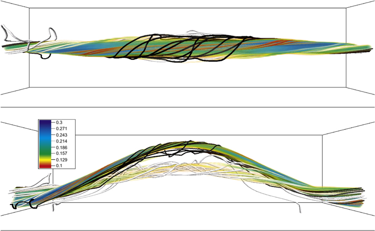
Figure 1. Illustration of the Ω-loop structure. The magnetic field strength is shown in three dimensions with a blue–yellow color scale for simulation  at t = 62 including a top view (upper panel) and a side view (lower panel). Different sets of magnetic field lines are also shown, with colors explained in the text. The accompanying online figure allows 3D navigation: it has two iso-contours, a yellow semitransparent one at
  for better visualization of the tail of the tube, and one at
  to explore the head region and the same set of field lines as the figure.
Download figure:
Standard image High-resolution imageThe 3D view provided in Figure 1 can be completed through the time evolution of the cross section of the same tube presented in Figure 2 for times t = 13, 35, 48 and 62. In the figure, magnetic field strength (top row) and vorticity (bottom row) maps are drawn on a vertical cut that coincides with the midplane of the box perpendicular to the initial axis of the tube. We confirm that most of the magnetic flux is concentrated at the very top of the structure. The general appearance and evolution of the structures shown are strongly reminiscent of those described by Moreno-Insertis & Emonet (1996), Emonet & Moreno-Insertis (1998) and Cheung et al. (2006) using 2D simulations. We recall a few salient features obtained in those papers and reproduced here: in the initial stages (two leftmost panels), the rising portion of the flux tube has a mushroom shape, akin to an air bubble rising in water (e.g., Davies & Taylor 1950; Collins 1965; Parlange 1969; Wegener & Parlange 1973; Hnat & Buckmaster 1976; Ryskin & Leal 1984; Christov & Volkov 1985). Within the ascending portion of the tube, vorticity is generated at the boundary layer between the tube and the ambient flow, in fact with opposite sign on the either side of the head (bottom row in the figure). Magnetic flux is dragged along the sides of the tube into a trailing pair of counter-rotating vortices. Later in time the wake is fragmented into smaller and smaller vortices because the Reynolds number increases in time due to the expansion of the tube (Cheung et al. 2006). The AMR device allows to see this fragmentation in much more detail than could be obtained in the original work of Emonet & Moreno-Insertis (1998). Inside the head of the tube, on the other hand, the plasma and magnetic field are executing a twisting oscillation, with small velocity compared to the global rise speed. This description of the time evolution of the flux tube structure generally applies to other simulations with comparable levels of refinement even when the twist and curvature vary. The cases with untwisted flux tubes, instead, follow a somewhat different pattern and their evolution is described in the following.
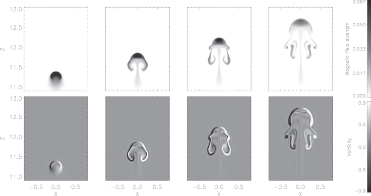
Figure 2. Longitudinal component of the magnetic field (top) and of the vorticity (bottom) are shown in grayscale in a xz section at the apex of the Ω-loop for simulation  at times 13, 35, 48, and 62, from left to right respectively.
Download figure:
Standard image High-resolution imageAn example of a simulation for an initially untwisted Ω-loop with a relatively high Reynolds number is experiment  shown in Figure 3. The appearance of the tube in the early phase (leftmost panel) resembles the 2D simulations by Schüssler (1979) and Longcope et al. (1996). After rising a distance of roughly one to two initial tube diameters, the tube has split into two counter-rotating vortex rolls. As the magnetic structure continues its rise, the top of the structure is pressed by the ambient flow into a horizontal bar shape. Thereafter, the bar is disrupted by an instability producing small vortices, possibly a Rayleigh–Taylor instability as described by Tsinganos (1980). This process spawns a flux tubelet emanating from the top of the tube (3rd and 4th column of the figure). As the tubelet rises above the main portion of the tube, it suffers a similar fate as the original tube, in that it splits into two counter-rotating rolls. In both cases, when a pair of counter-rotating rolls has been created, their sideways separation from each other is due to the action of the aerodynamic lift (Longcope et al. 1996). This whole phenomenon is probably also the reason for the structures shown in the 3D simulation of Dorch & Nordlund (1998, see their Figure 3, middle row), which are reminiscent of what we obtain here.

Figure 3. Longitudinal component of the magnetic field (top row) and of the vorticity (bottom row) are shown in grayscale in a xz section at the apex of the Ω-loop for simulation  at times 18.2, 39.6, 54.5, and 64.6, from left to right respectively. The black contours shown in the top-third panel are the different AMR levels, i.e., where the tube is, the AMR level is the highest, and the outer AMR level is the lowest.
Download figure:
Standard image High-resolution imageThe possible influence of the initial parameters on the bar structure is briefly explored in Figure 4, which compares maps of the longitudinal component of the magnetic field in the vertical midplane of the box for the three experiments carried out for tubes with no initial twist (λ = 0): apart from the Ω-loop experiment just described ( top panel), we present an experiment for a straight horizontal rising tube (
 middle panel) and an experiment like the one at the top but with no AMR (
 bottom panel). In all three experiments, the head of the tube expands, becoming horizontally elongated like a bar. This bar shape is possibly associated both with the larger amount of work needed to expand vertically (due to gravity) and with the lower pressure of the external flow on the sides due to the elementary Bernoulli effect (e.g., Parker 1979). The sideways expansion and deformation is not counteracted by magnetic tension due to the lack of twist in the tube. Within the bar, the motion is negligible except for the slow horizontal expansion of the tube in a similar way as happens in 2D simulations with twist, which have a negligible relative motion inside the head (Emonet & Moreno-Insertis 1998). The corresponding velocity shear between the tube and the outside plasma in the bar yields a vorticity distribution with opposite signs above and below it (as visible in the lower row of Figure 3). In the two cases with higher Reynolds number (top and bottom panels of Figure 4), the bar is later deformed with subsidiary wiggles. In fact the bar shows strong shear and has a density deficit in its interior, so the wiggles are possibly produced by a combination of the Rayleigh–Taylor and Kelvin–Helmholtz instabilities.

Figure 4. Cross-sectional structure of the tube at y = 0 for the three simulations without twist as follows:  at t = 64.6 (top panel),
  at t = 47 (middle panel), and
  at t = 72.7 (bottom panel). The longitudinal component of the magnetic field is shown in grayscale. The red arrows correspond to the projection onto the vertical plane of the relative velocity field with respect to the apex.
Download figure:
Standard image High-resolution image4. THE RETENTION OF MAGNETIC FLUX AS A FUNCTION OF CURVATURE, REYNOLDS NUMBER AND FIELD LINE TWIST
The central aim of this paper is to study which parameters influence the amount of flux lost by the rising Ω-loops using our 3D, high-resolution framework. From the possible parameters we select two which have been shown in previous studies to be particularly important in the process, namely, the field line twist (studied for rising horizontal tubes using 2D simulations by Moreno-Insertis & Emonet 1996; Emonet & Moreno-Insertis 1998), and the curvature of the Ω-loop (studied using low-resolution 3D simulations by Abbett et al. 2000). We then check if that dependence is substantially modified when increasing the spatial resolution (as done in 2D by Cheung et al. 2006).
There are various ways to measure the flux loss and the tube fragmentation. One method was developed by Moreno-Insertis & Emonet (1996) and Emonet & Moreno-Insertis (1998), who measure the amount of flux inside the main body of the tube (i.e., excluding the rolls in the wake and the tail) and compare it with the flux of the initial tube. Longcope et al. (1996) and Abbett et al. (2000), on the other hand, measure the sideways expansion of the vortices resulting from the splitting of the initial tube. We follow the first method and calculate the magnetic flux retained within the head of the tube at the apex of the Ω-loop ( ). To that end, we choose representative snapshots for each experiment and integrate the value of By in the region inside the head of the tube; for this measurement, we define the latter as the region where
  where
where  is the equipartition value with the kinetic energy:

For simulations with low AMR, we use a less strict condition, namely,  since the evolution of the tube leads to large relative kinetic energy with respect to the apex and in some cases, as shown later, the main body of the head of the tube remains together (see Section 4.3 for details). That value is subtracted from the total longitudinal flux in the tube at the initial time and the result is used as an approximation for the flux loss from the tube for the given run.
4.1. Dependence of Flux Retention on Tube Curvature
A particularly interesting dependence to explore is with the curvature of the axis of the rising tube. Abbett et al. (2000) reported that, in the 3D case of rising Ω-loops, the fragmentation of the rising tube was smaller the larger the curvature of the loop axis. Given the early date of all those results, the spatial resolution available to them was quite limited, specially the 3D ones. Our approach with AMR allows for much higher spatial resolution (hence a much larger Reynolds number). In the following we would like to test the flux loss dependence on curvature for different AMR regimes.
Figure 5 (left panel) displays a plot of the flux retained in the head of the tube,  as a function of the curvature parameter χ for simulations with a common value of the field line twist, namely, λ = 1/8. We have linked with lines the experiments with the same AMR level. For the lowest AMR level (dashed line), we find that flux retention increases with curvature, as reported by Abbett et al. (2000). In fact, comparing the cases with the extreme values of curvature (
 i.e., horizontal tube, left end of the curve and
  right end of the curve) we see a difference of close to 60% in the amount of flux retained in the head of the tube. Yet, going to cases with higher levels of AMR we see that the effect of curvature diminishes: the dashed–dotted line (for AMR = 1) shows a much less marked dependence, while the cases with the highest AMR (dotted line) show very little dependence with the curvature parameter. The amount of flux retained in those cases is in the range 40%–60%, which, as we will see in the next subsection, can be taken as representative for the value of twist used in all simulations in this figure.

Figure 5. Left panel:  plotted as a function of the curvature parameter (χ−1) for simulations with AMR = 0 (+ symbols, dashed line), AMR = 1 (
 dotted–dashed line) and AMR = 2 (*, dotted line). The cases with χ−1 = 0 correspond to 2D simulations. All cases considered in this figure have magnetic twist λ = 1/8. Right panel: magnetic flux retained within the head of the tube (
 ) as a function of Reynolds number for the same experiments as on the left panel. Also here, the lines link cases with the same level of AMR (namely, from left to right: AMR = 0, 1, 2).
Download figure:
Standard image High-resolution imageThe same trends as described above for the left panel of Figure 5 are revealed in the right panel which shows the effective Reynolds number against the amount of flux retained (the line style indicates the same values of the AMR used in the left panel). By comparing the two panels we see that, in the low AMR regime, the effective Reynolds number is highly dependent on the curvature. For the high AMR cases, instead, the effective Reynolds number, as well as the flux retained, are only weakly dependent on the curvature. The behavior and properties of the tube for low and high diffusion regimes are clearly different. For AMR = 0, the Reynolds number increases with curvature because of the variation in the size of the tube head. Instead, when using a higher number of AMR levels, the Reynolds number is seen to increase basically through the decrease in the width of the boundary layer.
In summary, we are able to reproduce the dependence of flux retention on curvature as reported by Abbett et al. (2000) only when the system is sufficiently diffusive. When higher AMR is used and sufficiently high-Re is achieved, the dependence of these properties on curvature is substantially diminished. We tentatively conclude that the curvature does not play any major role when the diffusion is low enough.
4.2. Dependence of Flux Retention on Twist
Here we would like to focus on the twist itself. Figure 6 shows  as a function of the field line twist for λ between 0 and 1/4. On the basis of the results of the previous section, we concentrate here on the cases with the highest AMR level (hence, with the highest Reynolds numbers). The lines link cases with the same value of the curvature parameter, namely, from the case with highest curvature (
 triangles, green line) through
  (asterisks, black line) and
  (squares, orange line), down to the cases with horizontal tubes (
 crosses, blue line). For comparison, we are also overplotting the corresponding 2D results of Cheung et al. (2006, their Figure 5), shown here with diamonds linked by a red line: those values were calculated with a much higher level of AMR (hence, of the Reynolds number) as was possible in the 3D calculations of the present paper. We also note that none of our 3D calculations in the figure are started with strongly twisted tubes: taking the highest twist used in the figure, λ = 1/4, and the pitch value given in Section 2.2, we see that the field lines only complete some 3.5 turns in the whole length of the box along the y-direction for the experiments with box size 10.4.

Figure 6.
 as a function of field line twist λ. The cases shown are: 2D experiments, i.e.,
  (+ symbols, blue line); experiments with
  (
( , orange line);
  (*, black line);
  (
( , green line). All the foregoing experiments cases were calculated with the highest AMR level. For comparison, 2D results from Cheung et al. (2006) are also plotted (
 red line).
Download figure:
Standard image High-resolution imageA clear result from Figure 6 is that, for each given fixed curvature,  dramatically increases with increasing magnetic field line twist following a pattern of the general shape obtained by Moreno-Insertis & Emonet (1996, their Figure 3) and Cheung et al. (2006) irrespective of the curvature of the Ω-loop. We note that the results of the 3D experiments for each λ cluster around a single value: the major deviation from this behavior appears for the smallest value of the twist (λ = 1/16), but even there the percentage of flux retained is less than a factor two difference between the different cases. This reinforces the conclusion reached in the last section that above a spatial resolution threshold the curvature of the Ω-loop is not the primary factor determining the amount of magnetic flux retained by the rising tube. The possible variation when going to higher resolution levels can be gauged by comparing the 2D results shown in the figure (crosses, red line) with those of Cheung et al. (2006): for λ = 1/4, for instance, the high-Re results are a factor roughly 1.2 above the moderate-Re ones.
4.3. Multi-parametric Study of the Tube Structures
We study in the following the variation of the cross-sectional structure of the rising magnetized domain when changing the main parameters in the study while keeping the others fixed. We carry out three comparisons: dependence with the twist parameter for an Ω-loop with χ = 1.5 and the highest AMR level (Section 4.3.1); dependence with curvature for the twist parameter fixed at λ = 1/8 for calculations with the highest AMR (Section 4.3.2); and, finally, the same dependence but for calculations with no AMR (Section 4.3.3).
4.3.1. Twist
Figure 7 shows the distribution of the longitudinal magnetic field By in the xz plane at the apex of the rising tubes for various degrees of twist (λ) but fixing the curvature at χ = 1.5 and always using the highest refinement level (AMR = 2). As one would expect from Section 4.2, one sees a reduction in the size of the head of the tube for decreasing twist. Beyond that, however, our high-resolution calculations allow to discern the high level of substructure one obtains when going to less twisted cases. For those cases in which a head is maintained (i.e., the three cases with λ > 0), we see that the shedding of vortices to the wake takes place earlier in the lower-λ cases, with at least a few vortex-shedding instances having taken place in the λ = 1/8 and λ = 1/4 experiments at the apex. Given the absence of net global vorticity in the cross section shown in the figure, the shedding of vortices is symmetric and no classical Von Karman vortex street is formed behind the tube (Emonet et al. 2001), i.e., no instability leading to an alternation in the vortex shedding from either side develops for the duration of the current experiments. On the other hand, one sees that the elaborate structure shown in the bottom right panel here and studied in Section 3 (Figure 4) only develops for untwisted tubes: even the limited level of the transverse field of the case shown in the bottom-left panel is sufficient to suppress the development of the vortex tubelets issued forward from the central bar.
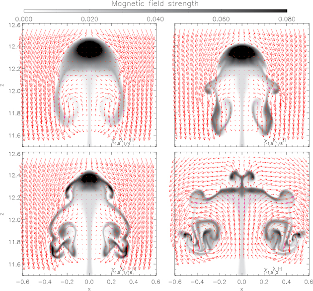
Figure 7. Dependence of the cross-sectional structure of the tube on the level of twist (λ). The layout is the same as in Figure 4. The simulations from left to right and top to bottom are  at t = 59 .2,
  at t = 54.5,
  at t = 59.2, and
  at t = 64.6.
Download figure:
Standard image High-resolution image4.3.2. Curvature—High AMR
In contrast to the strong changes seen when varying λ in Figure 7, the cross-sectional structure of cases with different curvature but constant λ and high AMR is remarkably similar (Figure 8). This property is in agreement with the fact that the amount of magnetic flux inside the tube ( ) varies only little with curvature when the spatial resolution is high enough (Section 4.1). A small difference between the various simulations shown in Figure 8, however, is that the horizontal expansion of the head of the tube is smaller the higher the curvature of the Ω-loop (i.e., the smaller the value of the χ parameter). This seems to be a consequence of the fact that the relative rise of the crest of the Ω-loops compared with their flanks entails a stretching of the tube along the axis which is larger the greater the curvature. This leads to an enhancement of the pressure deficit there which may counteract the tube expansion as it rises, even if to a limited extent.

Figure 8. Dependence of the cross-sectional structure of the tube on the curvature parameter (χ). The layout is the same as in Figure 4. The simulations from left to right and top to bottom are  at t = 62,
  at t = 56.6,
  at t = 54.5, and
  at t = 49.8. Compared to the dependence with twist, the tube structures are less sensitive to tube curvature.
Download figure:
Standard image High-resolution image4.3.3. Curvature—Low AMR
The structures seen in the previous two subsections fit well with the results on the magnetic flux retention by the head of the tube for the high-AMR experiments seen in the previous section (Section 4.2 and Figures 5 and 6). Looking at the dashed line in both panels of Figure 5, however, one wonders what may be causing the sensitive dependence on the curvature in the calculations without AMR. To check for this, we are showing in this section the cross sectional distributions of the longitudinal magnetic field for runs with different values of the curvature parameter χ when switching off the Adaptive Mesh Refinement (AMR = 0, Figure 9). For all experiments, we keep λ = 1/8, as also used for Figure 5.

Figure 9. Dependence of the cross-sectional structure of the tube on the curvature (χ) for simulations without adaptive mesh refinement (AMR = 0). The layout is the same as in Figure 4. The simulations from left to right and top to bottom are  at t = 74,
  at t = 73,
  at t = 55,
  at t = 73. In contrast to the relatively high Re regime, the structure of tube near the loop apex is very sensitive to the tube curvature.
Download figure:
Standard image High-resolution imageFigure 9 shows very different magnetic field distributions depending on the curvature. In this low-AMR regime, magnetic diffusion is sufficiently dominant to significantly debilitate the transverse field and hence the level of magnetic twist, and the ability of the tube to remain coherent. In the 2D case there is a clear separation of the tube into two vortex rolls which drift apart away from the central mid plane. In the 3D cases with high diffusion, instead, the two counterrotating vortices remain near the apex, where they are visible as two roundish dark features. The lift force would make those vortices move away from the central mid plane. However, in the figure we see that they stay nearer the apex the larger the curvature of the rising Ω-loop. This may be due to the fact that the stretching of the matter along the axis of the loop that accompanies the rise is more intense the larger the loop curvature. This leads to a relative gas pressure deficit at the apex which counteracts the motion of the vortices away from the midplane and which is more effective for more strongly curved loops. This helps the head of the tube maintain some identity during the simulated time interval in the low AMR cases with high axis curvature. In the cases with high spatial resolution of the previous section (Section 4.3.2, Figure 8), instead, the tension of the twisted transverse field inhibits any relevant dynamics inside the tube.
5. HORIZONTAL MOTION OF THE LEGS OF THE MAGNETIC LOOP DUE TO AERODYNAMIC LIFT
In the simplified 1D image of a rising Ω-loop as a thin, untwisted magnetic tube, sometimes the motion of the loop can be assumed to be contained in a vertical plane. To be sure, in the absence of effects associated with solar rotation and when the tube does not have any net vorticity anywhere along its length, all forces acting on the magnetized plasma point either in the tangential or normal direction to the tube axis, i.e., they cannot bring the tube out of a vertical plane if at any time it is completely contained in one. In the present paper, however, there may appear vortex forces associated with any net vorticity arising in any stretch of the tube, and they may carry the tube out of the initial vertical plane. In this section we show that this effect indeed takes place, in fact in an antisymmetric fashion for the two legs of the rising loop.
5.1. Preliminary Considerations
To obtain a first impression, we recall that the axis of the initial tube is contained in the vertical yz plane at x = 0; the sideways motion of the axis away from that plane can be studied by pursuing the intersection of the tube axis with the transverse vertical xz plane across either leg of the rising loop midway between the apex and the roots. Figure 10 shows the evolution of the intersection for the planes at y = ±2.7. In order to follow the center of the tube, we first locate it at the apex of the Ω-loop by searching for the minimum transverse magnetic field. Second, we trace the field line going through that point downward along the wings of the tube until they reach the chosen  plane. The figure corresponds to experiment
  in which, as we know from previous sections (e.g., Figure 7, top-left panel), the tube retains most of the flux in the rising body instead of shedding it to the wake. The legs (solid lines in Figure 10) actually move off the initial yz vertical plane in an antisymmetric way, following an inclined path with a superimposed oscillation sideways from it. The antisymmetry is also discernible in the 3D images displayed in Figures 1 and 11. The latter figure shows the y component of the vorticity for simulation
  using three different views. The upper panel shows a top view: we clearly see the flanks of the tube being displaced in opposite directions on either side of the crest. The two side views (middle and bottom panels) show antisymmetries also in the vertical position of the main body of the tube and in the wake.

Figure 10. Black and red solid lines: trajectory of the center of the tube in the vertical xz plane for simulation  at two equidistant positions with respect to the apex (red line at y = −2.7 and black line at y = 2.7). Dashed line: simple trajectory calculated with fixed values of vorticity and buoyancy as determined in the tube averaged within t = [13, 62] (see the text for details).
Download figure:
Standard image High-resolution image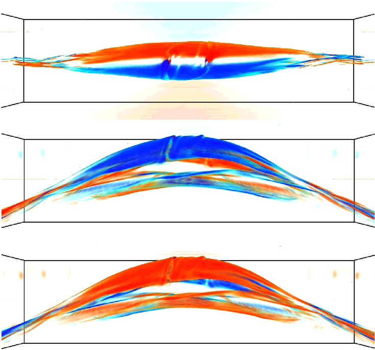
Figure 11. 3D images of the y component of the vorticity for simulation  at t = 65.95 (color-scale) are shown for a x-view (top panel) and the opposite x-view (middle panel) and z-view (bottom panel), where red is negative and blue is positive [−3.607, 3.607]. The wake has an antisymmetric behavior between the left and the right wings.
Download figure:
Standard image High-resolution imageThe basic reason for the right–left antisymmetry is that the legs of the loop carry net vorticity pointing along the tube axis and of opposite sense on either side of the apex. The force associated with a vortex line of strength  along its axis that moves with relative speed
  against the background leads to a lift acceleration given by
  × Γ (e.g., Lamb 1932; Saffman 1995; see also Longcope et al. 1996). Later on in this section we will be discussing why the legs of the tube develop net vorticity, in fact with vorticity vector pointing in opposite senses on either side of the tube head. Given that fact, and noting that the relative flow of the ambient medium seen by the tube points downward, one obtains a vortex force pointing in the x direction and, also here, in opposite senses for each leg of the rising tube.
The motion of the axis off the central yz vertical plane is thus a result of the lift force in combination with the buoyancy and drag forces. That sort of motion is particularly simple in the case of a rectilinear horizontal tube moving under the action of constant buoyancy, lift force and aerodynamic drag (Emonet et al. 2001) for small values of the dimensionless parameter

with CD the aerodynamic drag coefficient (taken CD = 2 below) and G, and R the average buoyancy acceleration, and the radius of the tube cross section, respectively: in that case, the motion of the tube has uniform velocity and the trajectory of its center is a straight line inclined to the vertical by an angle θ given by  Our tube is not horizontal and does not move uniformly; yet, for the sake of the comparison, we have included in Figure 10 (dashed line) such a trajectory for Ψ = 0.1 (correspondingly, θ = 18°), which is the average of Ψ calculated for the tube elements represented in the trajectory of the figure.
We can discern two main reasons for the appearance of net vorticity in the rising tube.
- (i)The action of the Lorentz force components associated with the varying amount of field line twist and cross sectional area one encounters when moving from the crest of the tube to the flanks.
- (ii)
Those two effects are discussed in turn in the following subsections.
5.2. Effect of the Inhomogeneous Distribution of Cross-sectional Radius and Field Line Twist along the Tube
Broadly speaking, twisted tubes tend to equalize twist along their length attempting to reach dynamical equilibrium: non-uniformities of the field line pitch along the axis promote plasma spin-up around the axis, e.g., in the form of a torsional Alfvén wave, that counteracts this lack of uniformity (see, e.g., Longcope & Klapper 1997; Longcope & Welsch 2000; Fan 2009). One can illustrate this process by studying the azimuthal component of the Lorentz force in simplified situations. Longcope & Klapper (1997) studied the equations that govern the evolution of a thin flux tube with twisted field lines and spinning motion around the axis. The thinness of the tube is meant in the sense that only the lowest-order terms need be retained in a radial expansion around the tube axis. Calling A the cross sectional area of the tube, they obtained an equation for the evolution of the angular momentum around the axis as follows:

where ∂ / ∂ l is the derivative along the axis of the tube, ω the spin of the tube around its axis, q the magnetic field torsion defined as  vA an average Alfvén speed in the tube cross section and γ2 a form factor related to the 2nd-order moment of the field distribution across the tube's cross section (see Longcope & Klapper 1997, Equations (33) and (A5)). From Equation (17), if the azimuthal component of the magnetic field varies along the axis in such a way as to make
  then a spin-up of the tube follows that tends to counteract this lack of uniformity.
Another comparatively simple situation is that of an axisymmetric flux tube with straight axis, now without imposing any condition on the size of the tube radius. In this case, one can easily split the azimuthal component of the Lorentz force into two parts.
- (a)The variation of the azimuthal field component as one slides in the axial direction leads to a radial component of the electric current. The latter, when combined with the axial field component, causes a force in the azimuthal direction, i.e., an axial torque. This leads to spin-up (i.e., to change of the axial angular momentum per unit mass) that tries to make the twist uniform.
- (b)For tubes with non-uniform cross section, the radial field component combined with the axial electric current that generally flows in twisted flux tubes leads to another component of the force in the azimuthal direction, i.e., again, to an axial torque and to change of the axial angular momentum.
We further note that the axial angular momentum per unit mass at an arbitrary radius of the simple axisymmetric tube is equal to the integrated amount of vorticity in the circular cross section of that radius.
In our simulations we can use neither one of the simplified avenues just discussed: the magnetic tube is not thin; concerning the second simplified approach, the axis of our tube is not straight and the initial axisymmetry is not strictly conserved along the evolution. However, examining the results of the simulation we can clearly conclude that the expansion experienced by the top part of the tube leads to a local minimum of the azimuthal field component and of the pitch angle at the apex inside of the main body of the tube (as apparent in Figure 1, red field lines ). Also, as expected from ideal MHD considerations, we see that the tube maintains along time the negative helicity configuration of the initial condition. Those facts, combined with the simplified considerations given in (a) above, allow us to expect an azimuthal component of the Lorentz force with positive (negative) sign in the left (right) wing of the tube. The corresponding torque leads to creation of axial vorticity in the tube pointing toward the apex, as measured in the experiment. Similarly, concerning (b) in the list of the previous paragraph, the cross section of the tube is maximum at its apex. One can check that the decrease of the cross section when moving down the flanks of the tube combined with the tube's negative helicity also leads to an axial torque that creates axial vorticity pointing toward the apex. We think that it is the vorticity created through these mechanisms, combined with the downward-pointing relative velocity of the surrounding medium with respect to the tube (as explained in Section 5.1), that results in a vortex force that causes the global sideways displacement in the x-direction shown in Figure 10.
5.3. Formation of a Von Karman Vortex Street
The vorticity changes associated with the shedding of vortex rolls from the wake of the rising tube (item (ii) in the list right before Section 5.2), and the corresponding changes in the lift acceleration also cause discernible perturbations in the motion of the tube. Figure 12 shows the trajectory of the tube axis on the transverse xz plane at fixed distances from the apex for various experiments with the highest AMR levels but with different values of twist and Ω-loop curvature. The time interval shown is t = 0 to t ∼ 70. All trajectories shown in the figure have an oscillating shape: the oscillation corresponds to the shedding of vortex rolls into the Von Karman street. The three solid lines, in particular, correspond to the three cases  (red),
  (blue) and
  (black), with the trajectories calculated on the vertical plane y = 3.1; we have provided velocity and field strength maps at the apex for those cases in Figure 7 (top-left, top-right and bottom-left panels, respectively). The total vorticity of the vortex rolls in the wake of those tubes increases for decreasing twist. Correspondingly, when the wake becomes asymmetric and vortex rolls are alternatively shed from either side of the tube into the Von Karman street, the associated elongation of the oscillations in the solid curves in Figure 12 becomes larger: this effect is quite marked for the low-twist case (black solid line) and marginally apparent for the red and blue curves. The actual asymmetry of the wake for the intermediate-twist case (
 i.e., the case for the blue solid curve in Figure 12) can be seen in Figure 13, with views provided for vertical cuts at the same instant (t = 65.95) and three different distances from the tube apex, namely, y = −0.762, y = −2.25 and y = −3.74; for comparison, one can also check the 3D volume rendering of the vorticity for this tube shown in Figure 11. Another effect apparent in the three solid curves of Figure 12 is that the global inclination of the trajectory is very small for the black curve and larger but rather similar for the red and blue curves. The global inclination of the trajectory is due to the effect discussed in the previous Section 5.2; correspondingly, when the twist is low (as for the case of the black solid curve in the figure) the vorticity generation due to this effect is also less important, and the motion away from the initial vertical plane less marked.
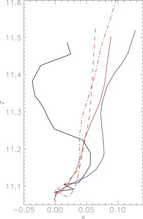
Figure 12. Trajectory of the center of the tube for simulations with twist 1/4 (red), twist 1/8 (blue) and twist 1/16 (black). The solid lines are the trajectories in the vertical plane y = 3.1 for cases with χ = 1.5; the dashed–dotted line is the trajectory in the plane y = 2.6 for the case χ = 1; finally, the dashed line is the trajectory in the plane y = 3.9 for the case χ = 2.1.
Download figure:
Standard image High-resolution image
Figure 13. A series of snapshots of the cross section of the longitudinal magnetic field are shown for the run  at t = 65.95, at y = (−0.762, −2.25, −2.25), from left to right, respectively.
Download figure:
Standard image High-resolution image
Still in Figure 12, we now compare the three curves in red, which explore the dependence with the curvature of the Ω-loop by choosing χ = 2.1 ( dashed line), χ = 1.5 (
 solid) and χ = 1 (
 dashed–dotted) on the planes y = 3.7, y = 3.1, and y = 2, respectively. The choice of different y values for those cases is because of the smaller longitudinal size of the Ω-loop for larger curvature cases. We see that there are only minor differences in the oscillations and global inclination of those curves. This is in line with the results of Sections 4.1 and 4.3.2 where we saw that in the high-AMR experiments the cross sectional structure of the head of the tube and the amount of magnetic flux it retains is similar irrespective of the value of χ. Here we show that also the net vorticity generation and the vorticity loss to the wake do not seem to depend on the curvature to any important extent.
6. DISCUSSION AND CONCLUSIONS
We have carried out a set of 2D and 3D MHD simulations of buoyant magnetic Ω-loops rising through a stratified layer covering a range of values of the loop curvature (as measured through the χ parameter, with ![$\chi \in [1,\infty ]$](https://content.cld.iop.org/journals/0004-637X/814/1/2/revision1/apj519845ieqn122.gif) ), field line twist (
), field line twist (![$\lambda \in [0,1/4]$](https://content.cld.iop.org/journals/0004-637X/814/1/2/revision1/apj519845ieqn123.gif) ) and effective Reynolds number. We have reached comparatively high Reynolds numbers in the 3D experiments by using the AMR algorithm of the Flash code. From the present study, we argue that the evolution of Ω-loops can be quite different when we compare the high-diffusion cases (with Re ≲ O(10), say) to cases with Re ∼ O(100). In the more diffusive cases with up to a moderate level of twist (λ = 1/8), the rising tube does not evolve into the simple configuration of a rising compact head with a trailing wake. In those cases the evolution strongly depends on the curvature of the tube axis; the dependence is substantially diminished in the high-resolution, low-diffusivity cases. A clear example has been shown in the text (Figures 5, 8, and 9). In the low AMR regime (high diffusion, Figure 9) without curvature, the tube's head splits into two big counterrotating vortices which drift apart due to the lift force when the rising tube is horizontal; instead, in the case of an Ω-loop with high enough curvature, the vortices are kept in the neighborhood of the loop axis. This effect comes about through the gas pressure deficit created near the loop apex by the plasma expansion in the direction of the Ω-loop axis whereas the plasma does not expand in that direction when the tube rises keeping a straight, horizontal shape. That there is a large dependence on curvature in those of our experiments without AMR is concomitant with the results of Abbett et al. (2000), who found that a sufficient level of Ω-loop curvature can help maintain the coherence of the tube. In contrast, in the high AMR regime (low diffusion) for the same value of λ (Figure 8), the vorticity is concentrated in a thin boundary layer, no splitting of the tube's head into vortices is seen, and there are no important differences in the results of the experiment in dependence of the loop curvature.
) and effective Reynolds number. We have reached comparatively high Reynolds numbers in the 3D experiments by using the AMR algorithm of the Flash code. From the present study, we argue that the evolution of Ω-loops can be quite different when we compare the high-diffusion cases (with Re ≲ O(10), say) to cases with Re ∼ O(100). In the more diffusive cases with up to a moderate level of twist (λ = 1/8), the rising tube does not evolve into the simple configuration of a rising compact head with a trailing wake. In those cases the evolution strongly depends on the curvature of the tube axis; the dependence is substantially diminished in the high-resolution, low-diffusivity cases. A clear example has been shown in the text (Figures 5, 8, and 9). In the low AMR regime (high diffusion, Figure 9) without curvature, the tube's head splits into two big counterrotating vortices which drift apart due to the lift force when the rising tube is horizontal; instead, in the case of an Ω-loop with high enough curvature, the vortices are kept in the neighborhood of the loop axis. This effect comes about through the gas pressure deficit created near the loop apex by the plasma expansion in the direction of the Ω-loop axis whereas the plasma does not expand in that direction when the tube rises keeping a straight, horizontal shape. That there is a large dependence on curvature in those of our experiments without AMR is concomitant with the results of Abbett et al. (2000), who found that a sufficient level of Ω-loop curvature can help maintain the coherence of the tube. In contrast, in the high AMR regime (low diffusion) for the same value of λ (Figure 8), the vorticity is concentrated in a thin boundary layer, no splitting of the tube's head into vortices is seen, and there are no important differences in the results of the experiment in dependence of the loop curvature.
In parallel to the foregoing, as part of our parametric study we have considered the dependence of the fragmentation of the tube with the magnetic field twist, focusing on cases with high AMR and a fixed curvature value (Figures 6 and 7). The amount of magnetic flux retained in the head of the tube as a function of field line twist in our 3D simulations follows a pattern as reported in 2D studies in the past (Moreno-Insertis & Emonet 1996; Emonet & Moreno-Insertis 1998; Cheung et al. 2006): as the twist increases and as a result of the magnetic field tension, the tube's head is more rounded and loses less magnetic flux to the wake. For λ ≳ 1/8 the head of the tube retains in all cases in excess of ≈50% of the original magnetic flux (more than 70% for λ = 1/4). The cross section of the apex of untwisted tubes, in turn, develops into a bar-shaped structure along the rise. This bar is a result of a horizontal expansion that is not counteracted by magnetic tension and is observed in all simulations without twist regardless of the curvature of the axis and of the Reynolds number.
Another finding of this work concerns the flanks of those Ω-loops with sufficiently twisted field lines to rise keeping a coherent tube-like structure: we see the flanks move away from their initial vertical plane in an antisymmetric fashion. We argue that such antisymmetric horizontal drift comes about because those tubes develop a global vortical motion around the tube axis in each flank, with vorticity pointing toward the apex of the Ω-loop: the ensuing lift force then leads to the antisymmetric motion of the flank away from the initial vertical plane. The vorticity is generated as a result of the inhomogeneous distribution of field line pitch on magnetic flux surfaces as one slides along the loop downward from the apex. This inhomogeneous distribution of field line pitch is directly caused by the expansion of the rising tube segments and leads to an unbalanced Lorentz force in the azimuthal direction around the tube axis, i.e., to a torque that makes the tube rotate around its axis, with associated generation of vorticity. Fan (2008) found that, when seen from above, the head of the rising Ω-loops in her experiment was increasingly tilted with respect to the direction of the tube in its original vertical plane. Considering the Maxwell stresses exerted on the end cross sections of a tube segment, she explained the tilt through the lack of compensation of the torque of those stresses when the segment is at or near the apex of the loop. Instead, no tilt is produced for a straight tube. We believe the physical process leading to the antisymmetric behavior of the flanks in our rising Ω-loop to be different to the one described by Fan (2008). In fact, the mechanism explained in Section 5.2 and summarized just above does operate also for straight tubes with varying cross-sectional radius as one slides along the tube axis. Also, the motion of the flanks in our case is an indirect effect of the Lorentz force: the latter generates vorticity in the tube which then leads, via the lift force, to the motion off the vertical plane.
The motion of the flanks off their initial vertical plane is accompanied by an oscillatory pattern (Figures 10 and 12). The oscillation is due to the shedding of vortex rolls to the wake and the corresponding creation of a Von Karman vortex street. We find that the amplitude of the oscillation increases as one considers less twisted tubes, because the rolls shed to the wake are larger and carry more vorticity the less twisted the initial tube. In contrast, there is no important dependence of the amplitude of oscillation with the curvature of the head of the Ω-loop. In the papers by Emonet et al. (2001), Cheung et al. (2006) the formation of a Von Karman street had been reached by imposing a net vorticity inside the tube at the beginning of the experiments. In the present case, the net vorticity is generated self-consistently through the mechanism indicated in the previous paragraph and in Section 5.2 and the vortex shedding thus follows naturally. The 2D simulations of rising buoyant tubes by Hughes et al. (1998) had an adaptive grid refinement algorithm and reached high Reynolds numbers, like, e.g., 4 103. They showed the trajectory of the axis of the rising tube in a vertical plane and compared it with that obtained in an experiment with a higher level of diffusion: the former showed what can be described as epicycles superimposed on a smooth trajectory (see their Figure 3). From the figures in their paper one gathers that vortex shedding was taking place in their experiment. Emonet et al. (2001) showed that trajectories for tubes with a high level of vorticity (more precisely, for a high value of the ratio defined in Equation (16)) could show epicycles and be far from simple, smooth sinusoidal paths. In three dimensions it is difficult to reach Reynolds numbers of a few thousand. On the other hand, as shown in the present paper, the extrapolation of 2D results to three dimensions is not straightforward since, among other things, the sideways motion of the tube can be countered by the Lorentz force associated with the tension of the longitudinal field component. The final answer to the evolution of 3D tubes must await the use of codes that allow experiments with very low diffusivity.
A natural extension of the current work would be to the case of magnetic ropes rising across a spherical shell mimicking the solar convection zone, i.e., at least using an unperturbed stratification closer to that of the actual solar convection zone and spherical geometry. Attempts in this direction have been made by Fan (2008) or, including self-consistent large-scale convection flows, by Jouve & Brun (2009), Jouve et al. (2013), Pinto & Brun (2013). As numerical methods and computing facilities improve, it will be possible to reach Reynolds numbers in that kind of experiment well above 100, in which the effects shown in this paper should become apparent. In fact, the phenomenon of flux tube splitting, and the influence thereon of the field line twist and curvature of the loop axis, could be preserved also in the presence of convection flows since they are essentially associated with the internal flux tube dynamics (barring effects associated to regions of strong shear in the convective cells). In any case, the dynamics of magnetic tubes moving in 3D environments is complicated enough to have to await the actual numerical experiments to decide on the approximate validity or otherwise of the simplifying assumptions made in this paper.
The authors acknowledge the support by the Spanish Ministry of Economy and Competitiveness through projects AYA2011-24808 and AYA2014-55078-P and by the European Commission through the SOLAIRE Network (MTRN-CT-2006-035484). J.M.S. is supported by NASA grants NNX11AN98G, NNM12AB40P and NASA contracts NNM07AA01C (Hinode), NNG09FA40C (IRIS), and NNX14AI14G (HGCR grant). We gratefully acknowledge the resources, technical expertise and assistance provided at the MareNostrum (BSC/CNS, Spain) and LaPalma (IAC, Spain) supercomputer installations, Notur project, and the Pleiades cluster through the computing project s1061 from the High End Computing (HEC) division of NASA as well as the computer and supercomputer resources of the Research Council of Norway through grant 170935/V30 and through grants of computing time from the Programme for Supercomputing. The FLASH computer code used in this work was in part developed by the DOE-supported ASC/Alliance Center for Astrophysical Thermonuclear Flashes at the University of Chicago. For 3D visualization UCAR's VAPOR package (Clyne et al. 2007;http://www.vapor.ucar.edu) and Tecplot software were used. Thanks are also due to S. Guglielmino for help and discussions during this project and to M. Jin for his help with the 3D visualization of Figure 1 for the online version of the paper.
APPENDIX: THE DETERMINATION OF THE EFFECTIVE REYNOLDS NUMBER
Determining the effective Reynolds number of a simulation is not simple. For multidimensional experiments of rising flux tubes, the problem is alleviated by using the theory of boundary layer formation in flows around straight cylinders, which predicts a layer width of order D Re−1/2, with D the diameter of the cylinder. How well this law applies also to rising magnetic tubes in a stratified medium was studied in some detail by Emonet & Moreno-Insertis (1998). We follow those results in a similar way as Cheung et al. (2006) and assume that

where D here stands for the transverse size of the tube at a given time, Lb for the width of the (magnetic or viscous) boundary layer around it, and K is a calibration factor of order unity introduced in this paper and explained below. In order to calculate D, we first calculate the area A of the tube cross section by determining the domain where  with
with  given through Equation (15), and then specify
  This prescription works well for the simulations with medium and high AMR; for those in the low AMR regime the cross sectional area A is obtained through the condition
  We have chosen this criteria because the main body of the tube for simulations with high diffusion and enough curvature has two vortex rolls with considerably large velocities and still maintains the magnetic structure of the tube's head during their evolution (see Section 4.3.3). The last column in Table 1 shows the diameter calculated in this way for each simulation at time t ∼ 50. The boundary layer width, Lb, can be measured in different ways (Emonet & Moreno-Insertis 1998). In a reference system moving upward with the speed of the center of the tube apex, the external medium is seen flowing downward around the head. The transition between the velocity of the external medium and the tube interior occurs in an abrupt way precisely in the boundary layer. The best determination of the boundary layer width can be done by measuring vx along a vertical axis slightly offset by one grid point from the mid vertical axis of the tube head: Lb is determined as the width of the layer in which vx decreases from the external value to 1/e of it. The value obtained in this way for Lb typically spans about six grid cells for any level of AMR.
The seventh column in Table 1 lists the Reynolds number for each simulation at time t ∼ 50 using Equation (18) with K defined so as to allow comparison with the numbers given by Cheung et al. (2006). To that end, we note that the Reynolds number varies in time mainly because the tube diameter increases along the rise due to the decrease of the external pressure. The simulations by Cheung et al. (2006) reached larger Reynolds numbers than ours for the same spatial resolution because they calculated the Reynolds number at substantially later instants: their 2.5D simulations allowed them to include a domain spanning a larger number of pressure scale-heights than in the present paper. Therefore, in order to facilitate the comparison between the two studies, we decided to calibrate our estimates of Re to the values quoted by Cheung et al. (2006). We choose a 2.5D simulation in our set for which the refinement level is the same in both studies. Comparing the value of Re obtained by us and the number quoted by Cheung et al. (2006) at a later time, we find a factor 1.75 between them. We then multiply the values of Re in our experiments with that factor, i.e., we set K = 1.75 in Equation (18). This recalibration is justified for our horizontal tube (i.e., 2.5D) experiments for the reasons mentioned, but, of course, only leads to a rough estimate of the Reynolds number at later times for the general 3D cases.
In our simulations, the viscous and magnetic boundary layers to have similar thickness, about 6 grid cells, indicating that Re ≈ Rem. This is because the viscous and magnetic diffusion stem from the numerical truncation inherent in the scheme.
While the maximum refinement level has a direct impact on Re, it is not the only relevant factor. Other properties of the tube, for instance, the twist and the curvature, affect the evolution of the tube and thus play indirect roles on the effective Reynolds number achieved by the simulation. In fact, the twist and the curvature can change the size of the tube's head such as is described in more detail in our results (see as well the sixth, seventh and tenth columns in Table 1).