


ABSTRACT
Interstellar dust (ISD) in the solar system was detected in situ for the first time in 1993 by the Ulysses dust detector. The study of ISD is important for understanding its role in star and solar system formation. The goal of this paper is to understand the variability in the ISD observations from the Ulysses mission by using a Monte Carlo simulation of ISD trajectories, with the final aim to constrain the ISD particle properties from simulations and the data. The paper is part of a series of three: Strub et al. describe the variations of the ISD flow from the Ulysses data set, and Krüger et al. focus on its ISD mass distribution. We describe and interpret the simulations of the ISD flow at Ulysses orbit for a wide range of particle properties and discuss four open issues in ISD research: the existence of very big ISD particles, the lack of smaller ISD particles, the shift in dust flow direction in 2005, and particle properties. We conclude that the shift in the dust flow direction in 2005 can best be explained by Lorentz force in the inner heliosphere, but that an extra filtering mechanism is needed to fit the fluxes. A time-dependent filtering in the outer regions of the heliosphere is proposed for this. Also, the high charge-to-mass ratio values found for the heavier particles after 2003 indicate that these particles are lower in density than previously assumed. This method gives new insights into the ISD properties and paves the way toward getting a complete view on the ISD from the local interstellar cloud. We conclude that in combination with the data and simulations, also impact ionization experiments are necessary using low-density dust, in order to constrain the density of the particles.
Export citation and abstract BibTeX RIS
1. INTRODUCTION
The solar system is located in a warm, dense cloud of gas and dust, the local interstellar cloud (LIC), and it travels in the direction of the G cloud (Redfield & Linsky 2008; Frisch et al. 2011). Because of its relative motion, interstellar dust (ISD) enters the solar system at velocities4 of about 26 km s−1. ISD represents typically 0.5%–1% of the mass of the clouds in the Milky Way (Frisch et al. 1999; Krüger et al. 2015). It plays a vital role in the evolution of the galaxy and the formation of planetary systems through cooling of dust clouds, which then collapse to form stellar and planetary systems. Also, ISD allows for formation of complex molecules in interstellar space, or of molecules like H2. Through studying ISD we learn about the history and formation of our own solar system.
1.1. Early Observations
Astronomical observations of the wavelength dependence of the extinction of starlight over kiloparsec distances, polarization and emission in the infrared, and complementary modeling led to several models of the size distribution and composition of ISD (Trumpler 1930; Mathis et al. 1977; Draine & Lee 1984; Weingartner & Draine 2001). These models generally show a power-law distribution with an upper limit on the biggest particles constrained by observational limits and by the abundances of the material in the gas phase (with the solar composition as a reference). From the depletion of elements in the gas phase measured in the absorption spectra of starlight, the ISD must contain mainly C, Mg, Si, Fe, O, and perhaps H (Draine 2004). Since we do not know exactly the local ISD size distribution and composition in the LIC, we take an (extrapolated) ISD distribution modeled by Mathis et al. (1977) as a reference power-law distribution in our studies (Sterken et al. 2013a). This is the so-called MRN distribution from Mathis, Rumpl, and Nordsieck. It is the most commonly used mass distribution, consisting of two particle populations with a power law of −3.5 and an upper limit of 0.25 and 1 μm for silicate and graphite, respectively. One must keep in mind that these models are based on observations over long kiloparsec distances whereas the LIC is very local, only a few parsecs. Thus, the size distribution of ISD in the LIC may look different from these models, and one of our goals is to come closer to a realistic original ISD size distribution in the LIC (Grün & Landgraf 2000).
1.2. ISD in the Solar System
Bertaux & Blamont (1976) predicted that ISD can enter the solar system and calculated the effect of the solar gravity and solar radiation pressure forces on the ISD flux. Levy & Jokipii (1976) predicted that these particles have a net electric charge, and therefore their trajectories would be influenced by the interplanetary magnetic field (IMF) via the Lorentz force. Based on this, they predicted that some of the particles with a high charge-to-mass ratio would be excluded from the solar system. Gustafson & Misconi (1979) and Morfill & Grün (1979) calculated ISD trajectories and concluded that there are phases of focusing and phases of defocusing of dust with respect to the solar equatorial plane. These phases depend on the 22 yr Hale cycle of the Sun.
In 1993, a major milestone in the local ISD research occurred when ISD in the solar system was unambiguously detected by the Ulysses dust experiment (Grün et al. 1993). The Ulysses dust detector is an impact ionization detector that measured the velocity and mass of the impacting particles through the velocity of the ions and electrons and the total impact ionization charge after an impact of a dust particle on the detector (Grün et al. 1992). The distinction between interstellar and interplanetary dust was possible owing to the exceptional orbit geometry of the Ulysses mission—out of the ecliptic plane and almost perpendicular to the incoming stream of ISD. Moreover, during the longest parts of the Ulysses orbit (only except for perihelion), the ISD came from the opposite direction of interplanetary dust, allowing an easier distinction between the two. Today, the Ulysses ISD data set from 1992 until 2008 is the most unique ISD data set, with over 900 detected ISD particles spanning almost a full Hale cycle, and is described in Krüger et al. (2015) for the mass distribution and Strub et al. (2015) for the ISD flux and flow direction. The flow direction is derived from the pointing direction of the instrument at impact.
These Ulysses data from 1993 until 2002 were thoroughly analyzed by Landgraf et al. (2000), and extensive modeling was done by the same author to better understand the data set (Landgraf 2000). Also Galileo—which carried a twin of the Ulysses dust detector—provided ISD data, along with Helios and Cassini (Altobelli 2004). An overview of papers related to in situ ISD observations and their data reduction is presented in Table 1 of Sterken et al. (2012).
1.3. Modeling the ISD Flow in the Heliosphere
From the fit of the modeled flux and the flux from Ulysses and Galileo data from 1992 to 1998, Landgraf et al. (2003) concluded that the bulk of ISD particles have sizes of about 0.3 μm, assuming compact astronomical silicates with density 2.5 × 10³ kg m−3 for the ISD material. Astronomical silicates are hypothetical materials with optical properties corresponding to those as determined from ISD by Draine & Lee (1984). The flux from 1992 until 1998 could be reproduced in simulations for particles with Q/m between 0.5 and 1.4 C kg−1.
Sterken et al. (2012) followed up on this work and did Monte Carlo simulations of the ISD trajectories for a whole range of material properties with a similar model (averaged IMF; see Section 2.2) in order to better understand the general flow and filtering of ISD in the solar system. The IMF was updated to have the heliospheric current sheet (HCS) rotation equal to the observed HCS rotation, but the standard model (sinusoidal HCS rotation) was still used to analyze the flow of ISD. In these studies, especially the Lorentz force leads to unexpected concentrations of dust at certain places in the solar system, depending on time. The updated ISD model was later used as a basis for inclusion in the ESA Interplanetary Meteoroid Environment for eXploration (IMEX) model, which is an engineering model for calculating the time-variable ISD flow and cometary dust streams to prepare future missions (Grün et al. 2013; Sterken et al. 2013b; Strub et al. 2013).
1.4. Influence of the Outer Boundaries of the Heliosphere
The influence of the heliopause (HP) on the ISD flux was calculated by Linde & Gombosi (2000) for the 1996 solar minimum, and they found a strong filtering for ISD smaller than 0.1 μm. Also Slavin et al. (2010) predicted a strong filtering at the HP for an IMF configuration with outward field structure ("positive field") in the northern hemisphere. Slavin et al. (2012) simulated the flow of ISD throughout the heliosphere boundaries and the inner heliosphere for both configurations of the IMF, but the effect of the changing IMF throughout the travel time of the ISD particles in the solar system was not taken into account. They concluded that particles as small as 0.03 μm can cross the HP. Although the results do not reflect the final distribution of ISD in the inner HP because of the lacking time dependence of the IMF, the authors did demonstrate that at the HP also focusing can occur, and that smaller particles can penetrate the HP at favorable configurations of the outer IMF.
1.5. A Shift in the Dust Flow Direction
Krüger et al. (2010) further analyzed the data of Ulysses and discovered an unexpected shift of 30° in the latitudinal direction of the dust away from the ecliptic plane with respect to its initial flow direction in 2005. This initial flow direction is assumed to be co-aligned with the neutral helium gas flow direction, supported by the argument that the overall dust direction from observations was found to be compatible with the helium flow direction (Baguhl et al. 1995; Landgraf 1998; Frisch et al. 1999) and that the main component of the dust velocity is determined by the high relative velocity of the solar system and the LIC. Finally, Strub et al. (2015) and Krüger et al. (2015) analyzed the complete ISD data set of Ulysses from 1992 February until 2007 November. They found that the small particles even have a larger shift in flow direction up to 50° in 2005.
1.6. Other Observations
Four other means of obtaining knowledge on the local ISD in the LIC are observations in the infrared, meteoroid observations, impact signatures picked up by spacecraft antennae, and sample return missions. Grogan et al. (1996a, 1996b) modeled the time-variable thermal emission of ISD with the aim to search for its signature in the Cosmic Background Explorer (COBE) and Infrared Astronomical Satellite (IRAS) data. Rowan-Robinson & May (2013) modeled the IR emission from the zodiacal cloud, including a steady component of the ISD from observations made by IRAS and COBE. They did not include the variations in ISD density in their models and conclude that there is "a need for a ground-based kinematic study of zodiacal dust" to test for this. The Herschel and Planck space telescopes have observed thermal emission and its evolution of dust in nearby molecular clouds, including cold and dense clouds, and the gas. ISD is often used as a tracer of their magnetic fields. Herschel data are also currently used in a survey of dust in different distant galaxies (Boselli et al. 2010). Although this dust is very far away, the link between in situ dust measurements and observations in the LIC, molecular clouds, or even other galaxies is important to get a full picture of the role of the dust in the universe.
Interstellar meteoroids were reported by Taylor et al. (1996), Hajdukova (1994), and Baggaley (2000), but much discussion remained about their true origin, and the results depended very strongly on measurement uncertainty (Hajduková et al. 2014). A maximum of about 20 ISD meteoroids were found in the data of the Japanese multistation video meteor network. These are macroscopic particles, typically larger than a millimeter.
Also radio and plasma wave instruments on STEREO detected ISD impacts (Belheouane et al. 2012): when the particles impact the spacecraft or the antennae, a cloud of plasma is generated from the dust and spacecraft material, which is then detected by the antennae. Calibrations of this mechanism were performed in the lab with different spacecraft materials (Collette et al. 2014). ISD detections using spacecraft antennae were also confirmed with the Wind/WAVES instrument (Malaspina et al. 2014).
In 2006, the Stardust mission returned a collector tray with contemporary ISD particles to Earth and started the "Interstellar Preliminary Examination (ISPE)": an effort to find and extract the first ISD particles, caught more or less intact in the aerogel, and analyze them for their chemical composition, crystallinity, size, and density. Two particles were found at the end of the track in the aerogel, and one track showed particle residues on the track walls but no end particle (Westphal et al. 2014). In the aluminum foils surrounding the aerogel, four craters were found with residues of ISD particles. The particles were diverse in chemical composition and crystallinity, were about 1 or 2 μm in size, and had a surprisingly low density of <0.4 g cm−3 and 0.7 g cm−3, respectively, for two of the particles (Westphal et al. 2014).
1.7. Open Questions
ISD in the LIC is fairly well characterized using the above-mentioned methods. However, still many questions remain open: (1) Why are astronomical observations and models of the dust mass distributions different from mass distributions derived from in situ measurements? (2) How does this comply to the constraints on the total mass of the ISD derived from abundances in the gas phase with respect to the Sun? (3) What causes the shift in dust flow direction in 2005 as reported by Krüger et al. (2010, 2015) and Strub et al. (2015)? (4) What are the characteristics of the ISD from the local interstellar cloud? (5) Can we fit the mass distributions and fluxes from astronomical observations and models, and what would we then learn about the dust particle properties?
In this paper we show and explain the simulated ISD flow for the Ulysses mission using the model of Sterken et al. (2012) and discuss the questions above in the context of the simulations and the Ulysses in situ ISD data. This is part of three related papers that aim at better understanding the complete Ulysses ISD data set, for fluxes, velocities, directions, and mass distributions throughout the whole mission (Krüger et al. 2015; Strub et al. 2015). The simulation program and the ISD flow characteristics are described in detail in Sterken et al. (2012). The filtering or enhancement of the ISD flux and changes in its size distribution throughout time are described for several places in the solar system in Sterken et al. (2013a). Those two papers give the background knowledge that is applied in this paper to understand the predicted fluxes, flow directions, and mass distributions at Ulysses.
We review the dust dynamics and assumptions of the model from Sterken et al. (2012) in Section 2 and then describe briefly the simulation results at the orbit of Ulysses in Section 3. A detailed description of the simulation results is given in Appendix
Throughout the paper we distinguish "big" particles from "small" particles at m ≈ 2 × 10⁻¹⁶ kg following the division in the Ulysses data from Strub et al. (2015). "Very big particles" or "the biggest particles" are generally micron sized and above. Because the density of the ISD particles is not yet constrained, an overview of particle masses with corresponding sizes for different densities is given in Table 1.
Table 1. Overview of Particle Masses (in kg) with Corresponding Radii (in μm) for Different Particle Densities
| Mass (kg) | Radius (μm) | Radius (μm) | Radius (μm) | Radius (μm) | Radius (μm) |
|---|---|---|---|---|---|
| ρ = 3.3 g cm−3 | ρ = 2.5 g cm−3 | ρ = 1.5 g cm−3 | ρ = 0.7 g cm−3 | ρ = 0.3 g cm−3 | |
| 10−13 | 1.93 | 2.12 | 2.52 | 3.24 | 4.30 |
| 10−14 | 0.89 | 0.98 | 1.17 | 1.60 | 2.00 |
| 10−15 | 0.42 | 0.46 | 0.54 | 0.70 | 0.93 |
| 10−16 | 0.19 | 0.21 | 0.25 | 0.32 | 0.43 |
| 10−17 | 0.09 | 0.10 | 0.12 | 0.15 | 0.20 |
| 10−18 | 0.04 | 0.05 | 0.05 | 0.07 | 0.09 |
| 2 × 10⁻¹⁶ | 0.24 | 0.27 | 0.32 | 0.40 | 0.54 |
Download table as: ASCIITypeset image
2. DUST DYNAMICS AND SIMULATION ASSUMPTIONS
2.1. Dust Dynamics
The trajectories of charged ISD particles in the solar system are shaped by solar gravity Fgrav, solar radiation pressure force FSRP, and the Lorentz force FL due to interaction with the IMF. The first two forces cause a steady axisymmetric ISD flow. They both scale with the squared distance to the Sun, and thus their ratio  can be seen as a constant ISD property that depends on particle morphology, density, material composition, and size. ISD particles with β = 1 move on straight lines "undisturbed" through the solar system. Interstellar particles for which the gravity is larger than the solar radiation pressure force (β < 1) move in hyperbolic orbits around the Sun and back into interstellar space, leading to a focusing cone of higher dust densities downstream from the Sun. ISD with β > 1 cannot travel closer to the Sun than a paraboloid-shaped zone owing to the high solar radiation pressure forces. Such particles cannot penetrate this so-called β-cone. Such a cone exists for each β-value, and thus studying the detection of ISD in different regions in the solar system allows us to learn about β and to indirectly constrain the particle properties. Figure 1 shows Ulysses's second polar orbit about the Sun and the approximate positions of these β-cones.

Figure 1. Ulysses's second orbit about the Sun (1998 until 2004) and the approximate positions of the β-cones in the ecliptic frame. The plots are drawn in the "interstellar dust frame," with the Z-axis equal to the solar rotation axis and the XY-plane equal to the solar equatorial plane. The X-axis is perpendicular to the Z-axis, and the XZ-plane is defined by the direction of the velocity vector of the dust. In the XZ-plane, the dust thus flows mainly along the X-axis, with an offset of about 7 5 in the Z-direction. The Y-component of the initial dust velocity vector is zero in this frame (Sterken et al. 2012).
Download figure:
Standard image High-resolution imageThe relationship between β and the particle size is called the "β-curve" and is determined by theoretical computations of scattering of electromagnetic radiation (Mie theory) or by experimental measurements (Gustafson 1994). Some examples of β-curves from Kimura & Mann (1999) and Draine & Lee (1984) are shown in Figure 2.

Figure 2. β-curves for several materials from Kimura & Mann (1999) and (in red) the adapted astrosilicates curve with βmax = 1.6. "Adapted astrosilicates" are the "astrosilicates" from Draine & Lee (1984) multiplied by a factor of 1.2 to have a maximum βmax = 1.6, in agreement with the results from Landgraf et al. (1999). Silicates usually have a β-value below 1, so the "adapted astrosilicates" are most probably silicates with other darker constituents. p is the amount of porosity with 0% for compact particles.
Download figure:
Standard image High-resolution imageThe third force included in the ISD trajectory calculations is the Lorentz force acting on charged particles that move through a magnetic field. The IMF strength, direction, and the particle charge-to-mass ratio Q/m determine the strength of the Lorentz force. In the solar system, the charge-to-mass ratio ranges typically between 0 and 10 C kg−1. Particles with higher charge-to-mass ratio are considered not to be able to penetrate the HP. The Lorentz force thus depends on the 22 yr Hale cycle, resulting in a focusing and defocusing of the ISD with respect to the solar equatorial plane. The flow is not axisymmetric anymore and nonstationary. Numerical models are needed to predict density and velocity.
The general flow characteristics of ISD in the solar system can be summarized as follows.
Very big (compact) particles (m > 5 × 10⁻¹⁵ kg) have low β < 0.5 and a negligible charge-to-mass ratio. They are concentrated near and downstream from the Sun (with respect to the flow direction) by gravitational focusing. Their flow is stationary and axisymmetric.
Small particles (m < 10−18 kg) also have low β-values (β < 0.5, for silicates) but have higher charge-to-mass ratios. The flow of these dust particles is time dependent and focused or defocused at the equatorial plane of the Sun or at higher latitudes depending on the phase of the 22 yr Hale cycle. In this paper, we refer to these two phases as "the focusing phase of the Hale cycle" when the particles are focused near the equatorial plane of the Sun and "the defocusing phase of the Hale cycle" when the particles are concentrated at higher latitudes. Very small particles cannot enter the solar system owing to the Lorentz effects at the HP and heliosheath (see Section 2.2.6).
Intermediate-sized particles can have β-values higher than unity, leading to a β-cone around the Sun in the flow direction where no such particles can enter. Depending on the charge-to-mass ratio of the particle and on the phase in the Hale cycle, this cone is modified in shape. By comparing Ulysses in situ measurements with modeling, the maximum β-value of ISD was determined to be between 1.4 and 1.8 (Landgraf et al. 1999).
Sterken et al. (2012) give a general overview of how the flow is modified and show several plots of the shape modifications of the β-cone and the focusing and defocusing in the solar equatorial plane and at higher latitudes above the equatorial plane.
2.2. Assumptions
Understanding the interaction between the ISD and the heliosphere is a complex problem where several assumptions have to be made. Some of the parameters can be held open and be constrained in an iterative process, while others are taken to be constant. Numerical simulations of the flow of ISD were performed under the following assumptions.
2.2.1. Forces and Simulation Grid
The simulation grid cells are cubes of 1.5 AU in length; the entire simulation volume is a box centered around the Sun of 22 × 22 AU. The velocities, fluxes, and directions are averaged out in one grid cell over the characteristic time for a nominal particle to cross the cell (about 100 days at a velocity of 26 km s−1). We have learned from the simulations of individual trajectories that a small fraction of the particles at the position of a spacecraft can come from a different direction in space than the main stream of the particles, for instance, particles with low β "returning" from their hyperbolic journey around the Sun, or particles with high Q/m that travel back because of high Lorentz force (this is called "mirroring" in Sterken et al. 2012). These fractions are usually small but become more important at the perihelia and downstream from the Sun with respect to the flow direction. It is thus possible that an individual ISD particle arrives from a considerably different direction than predicted here, and future simulations of the ISD flux at Earth shall take the dispersion in direction and velocity into account. Ulysses's orbital plane is almost perpendicular to the ISD flow direction, and the perihelia are removed from the analysis of the ISD data, so Ulysses does not pass through the regions where considerably more dust comes from another direction, and thus for Ulysses this fraction is small.
The forces considered in this work are solar radiation pressure force, solar gravity, and Lorentz force. Gravity of other planets is not taken into account as it only affects a small portion of the ISD trajectories. Other smaller forces than these three are disregarded too. Of these, the Poynting–Robertson drag is the biggest one (Altobelli 2004), but it is only important for particles passing close to the Sun. Particles passing closer than 0.1 AU can be captured by the Sun and become bound on very elongated (but shrinking) elliptic orbits with an aphelion of up to 2 AU for the first orbit (Jackson 2001). They can also be ejected from the solar system by high radiation pressure forces ("β-meteoroids") depending on the β-value they get after initial sublimation. However, since Ulysses flew mostly farther away from the Sun (the closest were the perihelia at 1.4 AU, which were excluded from the data anyway), we also did not take this into account.
2.2.2. Particle Charge
Our model assumes a constant charge for the particles on their path throughout the solar system. The rate of photoemission and the rate of charged particles picked up from the solar wind plasma both depend on the inverse square distance to the Sun, which—owing to secondary electron emission—leads to an equilibrium voltage of about +5 V for particles with radius 1 μm and larger in average solar wind conditions (Mukai 1981; Grün et al. 1994). Particles of radius 0.03 μm have a slightly larger potential, and particles with smaller radii than 0.03 μm decrease in potential with decreasing size (Mukai 1981). Kempf et al. (2004) found from in situ measurements with the Cassini Cosmic Dust Analyser that the charge of interplanetary dust particles near Saturn was about +5 V. The particle charge may fluctuate as a result of changes in temperature and density of the solar wind plasma and velocity. Slavin et al. (2012) simulated the surface potentials for compact silicate particles interacting with the plasma and radiation field thoughout the heliosphere. Inside of the termination shock (TS), near 90 AU and toward the heliosphere nose, the surface potentials of particles with radii 0.1–1 μm were found to be +5 to +9 V; smaller 0.01–0.1 μm particles have potentials of +8 to +15 V. The largest particles, with radii >0.18 μm, achieved their highest potentials in the hot inner heliosheath. All grains have potentials of an order of magnitude higher in the heliosheath when compared to potentials in the interstellar medium. Inside of the TS, grain potentials tend to vary by up to 30% between the heliosheath and inner heliosphere (Slavin et al. 2012, Figure 2). The boundary regions of the heliosphere thus lead to higher charges locally for even the larger particles, as was also calculated by Kimura & Mann (1998), who reported a potential of about +3 V throughout the heliosphere for silicates and carbon and an increase in potential up to +11 V for silicates in the boundary regions of the heliosphere. Ma et al. (2013) studied the equilibrium potential of dust aggregates in the heliosphere and found that particles made of small monomers can have up to twice the charge of compact particles, depending on the amount of monomers and their size. In this work we do not study the heliosphere boundary regions and thus assume a reasonable constant value of +5 V, in agreement with Mukai (1981) and Kempf et al. (2004). The simulations are done for a large range of particle properties (the β-Q/m parameter space), and a lower or higher particle equilibrium potential like in Kimura & Mann (1998) or Slavin et al. (2012) would roughly correspond to simulations for a slightly lower or higher charge-to-mass ratio.
In this paper, particles with a higher Q/m correspond to smaller, porous or fluffy particles. A fluffy particle refers to a particle that has a rough surface, like an aggregate, and thus a high surface-to-mass ratio. Porous particles refer to particles with a lower density but still with a rather smooth surface. Porous particles have a higher Q/m than compact particles because their mass is lower per surface area, but fluffy dust has even higher Q/m because of the small particle effect. Thus, a porous particle has the same surface potential U as a compact particle, but a fluffy particle has a higher surface potential (Ma et al. 2013).
2.2.3. Interplanetary Magnetic Field
The IMF in the simulations is averaged over one solar rotation like in the model of Landgraf (2000). This is a simplified but valid approach for particles not too close to the Sun or for particles that are not too slow, like ISD. Furthermore, a steady sinusoidal change in the tilt angle of the HCS with time is assumed. The model was improved to include the angles of the HCS as given by the Wilcox Solar Observatory (WSO; Hoeksema 2015), and also the nonaveraged magnetic field was implemented, but in this paper we use the simplest model of the IMF for reasons of computation time. The dates of solar maxima and minima for the simplified model and WSO data are summarized in Figure 3. The model where the HCS turns at a steady rate is depicted as a sinusoidal wave (three Hale cycles), and the focusing and defocusing phases of the Hale cycle, as well as the solar maxima and minima, are indicated. The HCS angles (from 0° to 90°) from WSO solar magnetic field observations are shown in the bottom plot of Figure 3. The solid and dotted lines depict two different computation methods from the raw data, where the solid line is the preferred method (see Hoeksema 2015 for details). Solar maxima, minima, and the dust phases (defocusing, focusing) are indicated for comparison with the idealized model used in our simulations.
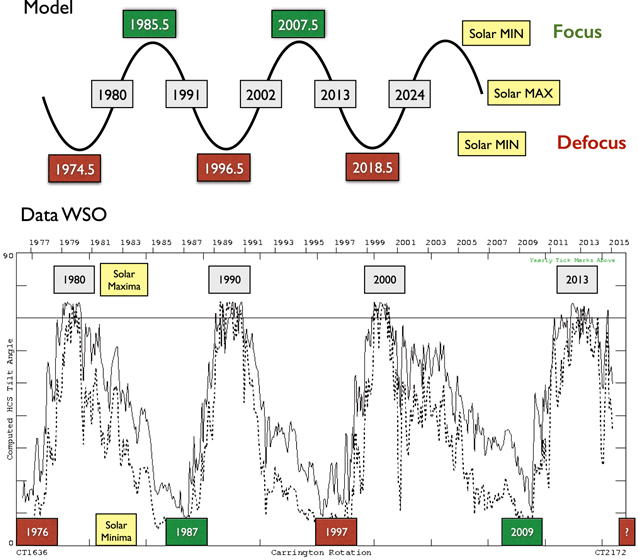
Figure 3. Overview of the dates when the interstellar dust is focused (green) and defocused (red) from the solar equatorial plane in the inner heliosphere, depending on the phase in the Hale cycle, for the model used in this paper (top panel) and as derived from Wilcox Solar Observatory solar magnetic field data (Hoeksema 2015; bottom panel). The bottom panel also shows the tilt angle of the heliospheric current sheet, being close to 0° at the solar minima and almost 90° at the solar maxima.
Download figure:
Standard image High-resolution imageTo illustrate the effect of the IMF model, we show in Figures 4 and 5 the simulations of the Ulysses data from 1992 to 2008 for the main population of ISD according to Landgraf (2000): β = 1.1 and Q/m = 0.6 C kg−1. We do this for the three different models (average Sun, rotating Sun, WSO Sun). The simulations agree well with the Landgraf simulations. Differences between the three models exist, but the influence of a missing HP will most likely be much more significant.
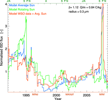
Figure 4. Simulated flux of ISD in the Ulysses frame and normalized to the undisturbed flow for three different models of the interplanetary magnetic field, and for β = 1.12 and Q/m = 0.84 C kg−1 (radius ≈0.3 μm). The three models give similar results. The model of the "Average Sun" uses an effective magnetic field value for calculating the Lorentz force, which is averaged over one solar rotation (25 days). The "Rotating Sun" model calculates the Lorentz force at each time step, so no averaging takes place. Last, the "WSO data + Avg. Sun" model is like the first but uses the data from the Solar Wilcox Observatory (Hoeksema 2015) for determining the rotation angle of the heliospheric current sheet. The first model was used for the simulation database for all β and Q/m values in this work, for reasons of computation time. The zigzag pattern is a result of the changing velocity of Ulysses in the period that it resides in one grid cell. In such a grid cell, there is only one value for the averaged simulated dust flux. The location of Ulysses is indicated on the top axis as "J/A" for Jupiter Aphelion, "S" for South polar pass, "P" for Perihelion, "N" for North polar pass, and "A" for Aphelion. The phase in the modeled Hale cycle is indicated on the bottom axis in red. "MINd" denotes the solar minimum of the defocusing phase, "MAXd/f" denotes the solar maximum between the defocusing and focusing phases, and "MINf" denotes the solar minimum of the focusing phase. The real Hale cycle has a solar maximum of the defocusing-to-focusing phase about 2 yr earlier (year 2000; see Figure 3).
Download figure:
Standard image High-resolution image
Figure 5. Simulated longitude and latitude of ISD flow at Ulysses in the ecliptic frame for the three different models of the interplanetary magnetic field, for β = 1.12 and Q/m = 0.84 C kg−1 (radius ≈ 0.3 μm). The three models give also similar results for the direction. The location of Ulysses and the phase in the modeled Hale cycle are indicated as in Figure 4.
Download figure:
Standard image High-resolution image2.2.4. Dust Properties
In previous studies (Landgraf 2000), ISD was mostly assumed to consist of compact silicates. In this study, we leave the particle properties—thus the relation between β, Q/m, dust mass, and size—open and rather approach the problem from the other side: by fitting the simulations to the data, we aim to constrain these two parameters (β, Q/m), which represent the particle properties: density, surface composition, and morphology (e.g., fluffiness). This paper prepares for this by analyzing first the simulations at Ulysses for all particle properties. For calculating mass distributions, a β-curve is assumed with maximum β of 1.6, since from analyzing the Ulysses data and the position of the β-cones, Landgraf et al. (1999) showed that the maximum β-value of the particles is between 1.4 and 1.8. The assumed density is 2.5 g cm−3, like normal compact silicates (note that the value used in Krüger et al. 2015 is slightly larger). The β-curves used in Section
2.2.5. Undisturbed Flow
The undisturbed initial flow of dust assumed in this study is a monodirectional homogenous flow coming from a direction of 259° ecliptic longitude, 8° ecliptic latitude, and flowing at a speed of 26 km s−1. The assumed direction is in agreement with the determination of the ISD direction from Ulysses dust data (Landgraf 1998; Frisch et al. 1999; Strub et al. 2015). The 1σ deviation of this flow is 259° ± 20° ecliptic latitude and 8° ± 10° ecliptic longitude. The neutral helium flow from the LIC was determined to come from a direction of about 255° ecliptic longitude and 5° ecliptic latitude at a speed of about 26 km s−1 (Witte 2004; McComas et al. 2015). These directions are well within the 1σ deviation of Landgraf (1998) and Frisch et al. (1999). The dust velocity was assumed to be equal to the Helium flow velocity (26 km s−1) because the velocity of detected ISD particles was comparable to this (Grün et al. 1993, 1994).
In 2006, the Stardust spacecraft returned particles captured in space from comet Wild 2, as well as a few particles that are likely to be ISD (Westphal et al. 2014). A preliminary analysis of these particles' trajectories has shown that the direction from which the three so far analyzed ISD particles came would fit better if their initial direction was 274° instead of 259° in longitude (Sterken et al. 2014). This is still within the 1σ uncertainty for the direction found by Landgraf (1998) and Frisch et al. (1999).
The assumed original size distribution of ISD particles entering the heliosphere is the MRN distribution (Mathis et al. 1977; see Section 1), extrapolated to larger and smaller sizes. The exact size distribution and limits in the LIC are unknown and, moreover, may be modified during the ISD propagation through the heliosphere boundary regions. Local variations in the dust size distribution were suggested by Grün & Landgraf (2000) because the big particles couple to the gas on much longer distance scales than the smaller ones.
2.2.6. Boundary of the Heliosphere
The heliospheric boundary regions (HP, heliosheath, TS) have different plasma properties and magnetic fields than the inner heliosphere. Particle charges there increase locally, and small particles may be filtered out at some times at the heliosphere boundaries (see Section 1) owing to the enhanced Lorentz force. The effect of the boundary regions of the heliosphere on the ISD flow is not taken into account in this study, but its possible role for the Ulysses fluxes and directions is discussed in Section 5.3.
3. SIMULATION RESULTS
In this section we summarize the simulation results for as much is needed to understand the discussion in Section 5. The detailed simulation results are described in Appendix
The simulated relative ISD flux at Ulysses is shown in Figure 6 for the biggest particles with radii on the order of a micron and bigger. This flux is normalized to the undisturbed flow, so the actual size distribution is not taken into account. The flux increases at every perihelion by a factor of 2–2.5, mainly as a result of the increased velocity of Ulysses at the perihelia. The fluxes of these big particles do not depend on the Hale cycle because of the low charge-to-mass ratio of the particles, and thus the fluxes are equal at every Ulysses orbit.
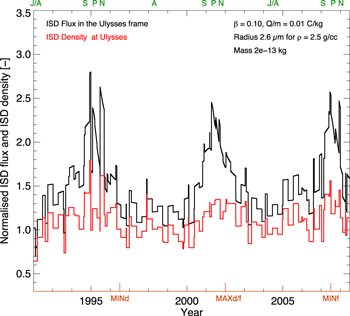
Figure 6. Simulated density and flux (in the Ulysses frame), normalized to the undisturbed flow, for the biggest particles (low β and near-zero Q/m, 2–3 μm radius). The density barely varies up to a factor of 1–1.5 at the perihelia (1.3 AU) owing to gravitational focusing, while the flux increases by a factor of 2 to 2.5 because of the faster velocities of Ulysses at the perihelia (the Ulysses orbit ascending node is approximately −22°, whereas the ISD incoming longitude is 79°). The zigzag pattern in the flux is due to the Ulysses velocity in combination with relatively big simulation grid cells of size 1.5 AU and an average relative error of about 20%. The location of Ulysses and the phase in the modeled Hale cycle are indicated as in Figure 4.
Download figure:
Standard image High-resolution imageFigure 7 shows the relative flux for different particle sizes. The influence of the Lorentz force and thus the Hale cycle becomes more obvious with decreasing particle size: the fluxes at the second perihelion (2001) are reduced in comparison to the other two perihelia (1995 and 2007) because of the defocusing phase of the Hale cycle. The combination of solar radiation pressure force, gravity, Lorentz force, and the Ulysses velocity vector with respect to the ISD velocity vector leads to a difference in flux of up to a factor of 10 between, for instance, 1998 (aphelion + defocusing phase) and 2008 (perihelion + focusing phase). The lowest flux in the simulations is in 1998 for all particle sizes.

Figure 7. Simulated ISD flux (in the Ulysses frame), normalized to the undisturbed flow, for particles with different β-Q/m combinations corresponding roughly to particle radii of 0.7 (purple line), 0.4 (light blue line), 0.3 (green line), and 0.2 (red line) μm assuming a density of ρ = 2.5 g cm−3. The zigzag pattern is due to the Ulysses velocity in combination with relatively big simulation grid cells of size 1.5 AU and an average relative error of about 20%. The location of Ulysses is indicated on the top axis as "J/A" for Jupiter Aphelion, "S" for South polar pass, "P" for Perihelion, "N" for North polar pass, and "A" for Aphelion. The phase in the modeled Hale cycle is indicated on the bottom axis in red. "MINd" denotes the solar minimum of the defocusing phase, "MAXd/f" denotes the solar maximum between the defocusing and focusing phases, and "MINf" denotes the solar minimum of the focusing phase. Note that there is an increase in relative flux in 2005 for the small particles, but not for the big ones, as reported in Strub et al. (2015). However, a similar high flux of small particles before 1994 and in 1996 was not observed.
Download figure:
Standard image High-resolution imageThe β-cone is visible as a "gap" at the perihelia (Figure 7, red curve for β = 1.5 and Q/m = 1.5) because no particles with β = 1.5 can reach Ulysses so close to the Sun. The flux of the particles just before and after the β-cone of 1995 is higher because the dust is diverted toward higher latitudes (almost above the solar poles) through the defocusing mechanism of the Lorentz force. In 2008, there is a single peak in the flux at the perihelion because the dust is focused near the equatorial plane of the Sun (Figure 7, light green curve for β = 1.3 and Q/m = 1 C kg−1).
From these simulations we learn that the fluxes at Ulysses are most influenced by Lorentz force and the Ulysses velocity, except for dust with high β-values when Ulysses moves through the β-cones.
Note the increase in relative particle flux around 2005 for  = 1–3 C kg−1 and the very high fluxes of the same particles before 1995. This is not seen for big particles with very low
  . These fluxes in particular will be discussed in Section 5.3: the discussion on the shift in dust flow direction and the role of the heliosheath therein. Also note that smaller particles are more abundant in the ISM because of the power-law size distribution from astronomical observations. The variability of the small particles should thus significantly have more influence on the total flux at Ulysses than the variability of the largest particles, unless they are partially or largely filtered out at the heliosheath and the power-law size distribution is no longer valid after having passed the TS.
The impact velocities of ISD on Ulysses are mostly between 20 and 50 km s−1 and are shown in Figure 8. These are described in detail in Section

Figure 8. Simulated ISD velocities at Ulysses but in the ecliptic frame for particles with different β-Q/m combinations corresponding roughly to particle radii of 0.7 (purple line), 0.4 (light blue line), 0.3 (green line), and 0.2 (red line) μm (assuming a density of ρ = 2.5 g cm−3). The location of Ulysses is indicated on the top axis as "J/A" for Jupiter Aphelion, "S" for South polar pass, "P" for Perihelion, "N" for North polar pass, and "A" for Aphelion. The phase in the modeled Hale cycle is indicated on the bottom axis in red. "MINd" denotes the solar minimum of the defocusing phase, "MAXd/f" denotes the solar maximum between the defocusing and focusing phases, and "MINf" denotes the solar minimum of the focusing phase. The plot gives an indication of how the ISD velocity differs per location in the solar system, independent of the velocity of Ulysses with respect to the ISD flow. The concentrations of big dust and lack of small dust (red line) around perihelia are visible, which are a consequence of small and large β-values, respectively. Other variations than the cyclic ones (per orbit) are due to the changing interplanetary magnetic field within the 22 yr cycle.
Download figure:
Standard image High-resolution imageSimulated impact directions for the biggest particles (Q/m ≈ 0 C kg−1) are shown in Figure 9. The ISD flow longitudes and latitudes at the position of Ulysses are cyclic and change the most around the perihelia. These latitudes and longitudes do not depend on Ulysses's velocity because they are in the ecliptic frame. Figure 10 shows the ISD flow longitudes and latitudes at the position of Ulysses but for decreasing particle size. The latitudes for β < 1 are opposite in sign to those for β > 1. The Lorentz force causes the latitudes and longitudes not to be cyclic anymore, especially in the period from 2005 until 2008 for the smaller particles.
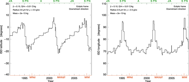
Figure 9. Simulated ISD flow direction latitude (left) and longitude (right) in the ecliptic frame for the biggest ISD particles (low β and near-zero Q/m, radius of 2–3 μm). These particles move on hyperbolic trajectories, and hence their latitude and longitude vary depending on the position of Ulysses. The latitude variations are the highest at the poles of the Sun, whereas the longitude variations are the highest at the perihelia, which is due to gravitational focusing of the flow. The location of Ulysses is indicated on the top axis as "J/A" for Jupiter Aphelion, "S" for South polar pass, "P" for Perihelion, "N" for North polar pass, and "A" for Aphelion. The phase in the modeled Hale cycle is indicated on the bottom axis in red, but the interplanetary magnetic field has no influence because the particles have a very low charge-to-mass ratio.
Download figure:
Standard image High-resolution image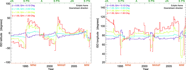
Figure 10. Simulated ISD flow direction latitude (left) and longitude (right) in the ecliptic frame for ISD particles with different β-Q/m combinations corresponding roughly to particle radii of 0.7 (purple line), 0.4 (light blue line), 0.3 (green line), and 0.2 (red line) μm.
Download figure:
Standard image High-resolution imageIn order to compare the simulations to the data of the Ulysses dust instrument in the next section, we need to transform ISD latitude and longitude in the ecliptic frame to directions in the spacecraft reference frame, and finally into the "rotation angle." This is the difference in angle between when a dust impact occurs and when the dust instrument points closest to the ecliptic north pole. The latter corresponds to 0° rotation angle, and a dust detector pointing parallel to the ecliptic plane corresponds to a rotation angle of 90°. A more detailed description of the spacecraft geometry and rotation angle is found in Grün et al. (1993), Landgraf (1998), and Strub et al. (2015).
Figure 11 shows the difference in rotation angle for these simulations with the rotation angle of the reference direction of the dust flow (259° longitude, −8° latitude). For the biggest particles, these differences remain below ~10° and occur mostly at the perihelia owing to their low β-values. For smaller particles, these shifts in rotation angle also occur at the perihelia, but also in some of the periods before or after the perihelia.

Figure 11. Shifts in rotation angle for different β-Q/m combinations corresponding to decreasing radii of particles (roughly 0.7, 0.4, 0.3, and 0.2 μm).
Download figure:
Standard image High-resolution imageThe mass and number distributions are simulated too by assuming the "adapted astrosilicate" β-curve. These are shown in Figure 12 for one day in every year of the Ulysses mission and in Figure 13 for the aphelia and perihelia only. These plots show the filtering of the ISD distribution with respect to an assumed initial power-law MRN distribution, and specifically how this filtering depends on time (Figure 12) and location (Figure 13) in the Hale cycle and solar system.

Figure 12. Simulated mass and number distributions per year for the Ulysses mission, assuming an MRN distribution as the "undisturbed" distribution (dashed line). The left plot shows the mass density per logarithmic mass interval in kg m−3. The middle plot shows the number density per logarithmic mass interval. The right plot shows the factor with which the MRN distribution was multiplied to obtain the distributions. This factor depends on time and place in the solar system.
Download figure:
Standard image High-resolution image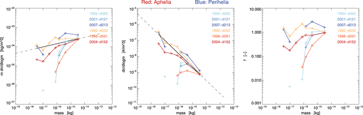
Figure 13. Same as Figure 12, but for the three orbits of Ulysses at the aphelia (red) and perihelia (blue), assuming an MRN distribution as the "undisturbed" distribution (dashed line).
Download figure:
Standard image High-resolution image4. Ulysses ISD DATA
The selection process and the data to which we compare the simulations in this paper are described in detail in Krüger et al. (2015) and Strub et al. (2015). The ISD data obtained from the Ulysses dust experiment are mass, impact velocity, and rotation angle. An ISD mass distribution was reconstructed by Krüger et al. (2015, Figure 5), and the variations of ISD flux and flow direction with time were analyzed in Strub et al. (2015).
For better understanding of the discussion in Section 5, we briefly introduce these data here. Figures 14–16 show the simulated ISD flux and rotation angle (colored lines) and data (bars) from Strub et al. (2015) for "big" and "small" particles, where the division between big and small is made at approximately m = 2 × 10⁻¹⁶ kg (Strub et al. 2015), corresponding to Q/m = 0.7 C kg−1 in our simulations, assuming a particle density of 2.5 g cm−3. In all four panels, the time bins are 30 days, and the bigger the error bars, the fewer particles are available per bin. The gray zones are the times when no data were analyzed because in those periods it is difficult to distinguish between interstellar and interplanetary dust. These periods are the three perihelia, and the smaller periods around 2004–2005, where Ulysses is close to Jupiter, and Jupiter dust streams were seen. These figures are further discussed in Section 5.3.
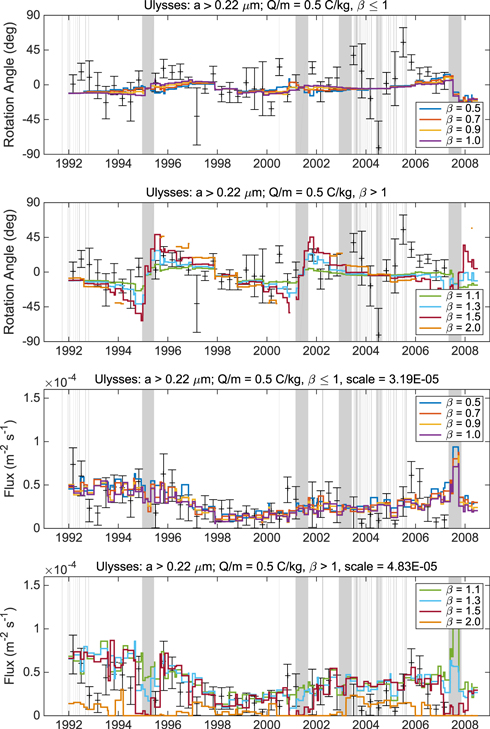
Figure 14. Simulations (colored lines) and data (plus signs with error bars) for the rotation angle (upper two panels) and normalized flux (lower two panels) for the big particles (m > 2 × 10⁻¹⁶ kg), Q/m = 0.5 C kg−1, and a range of β-values. The periods where no data were analyzed are indicated as gray bars at the aphelia of the Ulysses orbit and the Jupiter dust stream periods.
Download figure:
Standard image High-resolution image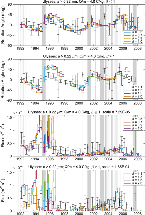
Figure 15. Similar to Figure 14, but for Q/m = 4 C kg−1.
Download figure:
Standard image High-resolution image
Figure 16. Similar to Figures 14 and 15, but for the small particles (m < 2 × 10⁻¹⁶ kg) and Q/m = 4 C kg−1.
Download figure:
Standard image High-resolution imageFigure 17 shows the ISD mass distribution from Krüger et al. (2015, bars) and the simulated mass distributions for different particle properties from this work. This figure is further discussed in Section 5.4.

Figure 17. Simulated mass density (per unit volume) averaged over the whole Ulysses mission (colored lines), and derived mass density from the Ulysses ISD data from Krüger et al. (2015; plus signs with error bars). The black line shows the "adapted astronomical silicates" with a density of 3 g cm−3 and a maximum βMAX = 1.6 (therefore it cannot be a pure silicate, but must contain also darker materials). The blue lines are "fluffy adapted astronomical silicates" using a β-curve that is derived from the "adapted astronomical silicate curve" and the porous silicates from Kimura & Mann (1999). The red curves represent carbon with different fluffiness, using a β-curve from Kimura & Mann (1999). Most of the mass is in the biggest particles. The "fluffy particles" are assumed to have a higher surface potential (Ma et al. 2013). An explanation of the effects of "fluffiness" and porosity on the mass density is given in the text.
Download figure:
Standard image High-resolution image5. DISCUSSION: SIMULATIONS IN THE CONTEXT OF THE OBSERVATIONS
In this section we discuss the simulations in the context of what is currently known about ISD from astronomical observations, in situ measurements, and the Stardust sample return mission. There are four unresolved issues on which we focus: (1) the excess of big ISD particles derived from in situ measurements compared to astronomical observations and constraints from cosmic abundances, (2) the lack of very small particles in the in situ measurements as compared to astronomical observations, (3) the observed shift in dust flow direction of ISD in 2005 as reported by Krüger et al. (2007) and Strub et al. (2015), and finally (4) the unknown particle properties—morphology, material, and density. We discuss each one of them with what can be proven to date, and we propose solutions to these questions from extended modeling and instrument calibrations in Section 6.
5.1. Big Particles
Classical ISD models derived from observations over kiloparsec distances (Mathis et al. 1977; Draine & Lee 1984; Weingartner & Draine 2001) typically have a cutoff in maximum particle size. This is 0.25 μm for silicates and 1 μm for carbon in Mathis et al. (1977). The maximum particle size is determined by observational constraints,5 by constraints in cosmic abundances (material observed in the gas phase cannot be in the dust phase, with the solar abundances taken as a reference), and by timescales of coagulation and shattering due to shock waves. However, single ISD particles with masses above 2 × 10⁻¹³ kg (>5 μm in diameter for compact particles and greater for porous particles) were measured with the Ulysses dust detector in the solar system (Krüger et al. 2015). Also the Helios data showed a large proportion of big interstellar particles (Altobelli et al. 2006). Apart from local variations in the dust size distribution as a proposed cause of these observations (Grün & Landgraf 1997), there is more recent astronomical evidence of micron-sized ISD particles (Gall et al. 2014; Wang et al. 2014, but not yet in the LIC), and also the Stardust mission returned two local ISD candidates with sizes of about a micron. The existence of low-density big particles helps to explain the observations and constraints (Dwek 1997; Li 2005), but it is not sufficient to explain the most massive ISD particles in the Ulysses ISD data set. Understanding the big particles is very important for determining the gas-to-dust mass ratio.
The simulations in this paper suggest that if these big ISD particles indeed exist, there should be an increase in the flux of big ISD particles around the perihelia by a factor of up to 1.5 owing to gravitational focusing (see discussion in Section
The big particles in the excluded data at the perihelia that are consistent with ISD directions and of high speed could possibly be ISD (Krüger et al. 2015; Strub et al. 2015). However, also very slow big particles were found around the perihelia (Strub et al. 2015), which may be caused by an unknown instrumental effect, or it could be cometary stream particles. The ESA-IMEX dust stream model can be used to further explore this topic, which is beyond the scope of this paper. We propose in Section 6.1 another possible explanation for the presence of very big ISD particles in the Ulysses ISD data set, which is based on the calibration of the dust instrument for compact versus fluffy or porous particles.
5.2. Smaller Particles
The mass distribution in Krüger et al. (2015, Figure 4) shows a large discrepancy between the mass densities of the smaller particles in the MRN model and the mass densities measured by Ulysses. This was understood in previous studies as a filtering by the solar radiation pressure force and the Lorentz force in the inner solar system and at the boundary regions of the heliosphere. The filtering in the inner solar system has been well characterized (Landgraf et al. 2000; Sterken et al. 2013a), but for the heliosphere boundary, the time-dependent effect of this filtering still needs to be implemented in studies like the ones by Slavin et al. (2012) and Linde & Gombosi (2000). Czechowski & Mann (2003) did the first such study and concluded that the alternating polarities of the IMF close to the HCS are favorable for particles to pass through the heliosheath.
The Hale cycle dependence of the flux of smaller particles is seen in the simulations and in the measurements and corresponds well to the analysis of Landgraf et al. (2003) if the bulk of the particles have indeed a 0.3 μm radius with β = 1.1 and Q/m = 0.6 C kg−1. Landgraf et al. (2003) concluded on this "bulk" population of 0.3 μm particles with smaller components of 0.4 and 0.2 μm particles by comparing ISD flux simulations with the Ulysses data.6 Only the flux was used for fitting the simulations to the data, and it only covered the period from 1992 until 2002.
Now not only are there three times as much data (1992 until 2008, Krüger et al. 2015), but we also consider the direction of the ISD flow (Strub et al. 2015). The general trend in the Hale cycle is still present in the full Ulysses data set, but the details cannot be fitted yet for the whole data set without additional modeling, as we explain in Sections 5.3 and 5.4. Note that in the data, particles smaller than 10−17 kg are measured before 1995 and after 2003 (Strub et al. 2015). In the simulations, these correspond to Q/m between 5 and 12 C kg−1 and even beyond.
5.3. Shift in Dust Flow Direction in 2005—Does the Heliosheath Play a Role?
In order to understand the shift in dust flow direction measured by Ulysses, we studied the simulations for 2005 in greater detail (see Figure 18). Details of these simulations are described in Section
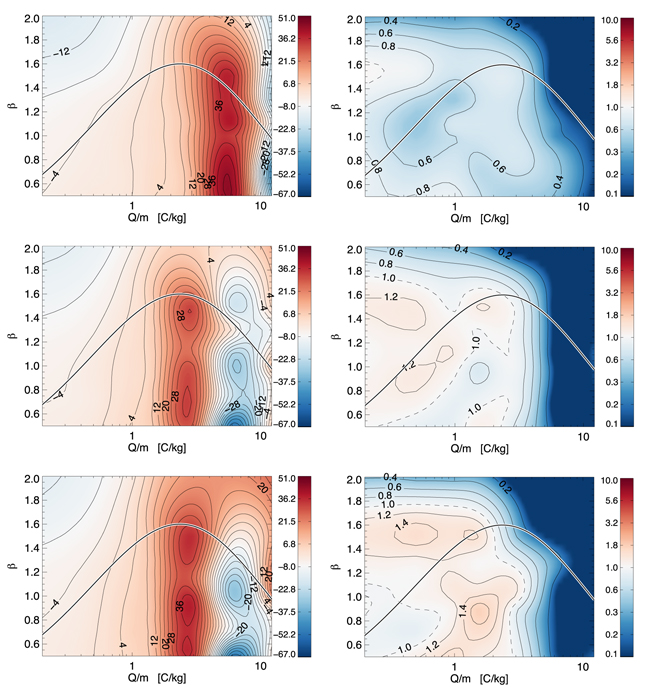
Figure 18. Simulated (downwind) ISD flow latitude in the ecliptic frame (left) and relative flux in the Ulysses frame (right) on 2005 April 1 (top), September 30 (middle), and November 15 (bottom) for all β and Q/m. The color bar on the right represents the simulated ISD flow latitude in degrees, where −8° is the undisturbed (downwind) inflow direction of the ISD. The color bar on the right shows the relative flux, with "1" as the value of the undisturbed inflow ISD flux in white. Red areas indicate a positive shift in dust direction; blue areas indicate a negative shift in dust direction. The line through the plot is the β-curve for the "adapted astronomical silicates," as introduced first in Sterken et al. (2012).
Download figure:
Standard image High-resolution image5.3.1. Shift in Dust Flow Direction of the Big Particles
In Section 4 we briefly introduced the Ulysses ISD data set from Krüger et al. (2015) and Strub et al. (2015). Here we compare the results of the simulations for the flux and rotation angle to the data. The colored lines in Figure 14 are the simulated rotation angles (top) and ISD fluxes (bottom) assuming particles with Q/m = 0.5 C kg−1 and different β-values. The data for big particles with masses m > 2 × 10⁻¹⁶ kg are shown as data points with error bars. These particle masses correspond to charge-to-mass ratios of Q/m ≤ 0.7 C kg−1 if we assume a particle density of 2.5 g cm−3. The rotation angles are in the Ulysses frame and the fluxes are in the ecliptic frame to allow for direct comparison with the data of Strub et al. (2015). The simulated fluxes are scaled to the data by matching their averages, and the scaling factor is indicated in the plot. The flux curves for particles with Q/m = 0.5 C kg−1 seem to fit well to the data indeed—until about 2003—which is in agreement with Landgraf (2000), who has shown that the bulk of the ISD particles have a radius of 0.3 μm with β = 1.1 and Q/m = 0.6 C kg−1. From our simulations, β = 1.3 would fit slightly better to the directions of the dust in the data. In any case, simulations for β < 1 and similar Q/m show too little variability in the rotation angles, and simulations for β > 1 but Q/m = 0.1 C kg−1 show a similar variability in the rotation angle, but too little variability in the flux to match well to the measured fluxes.
However, between 2004 and 2007, there is a clear increase and then a decrease in the flux data, which is not seen in the simulations for Q/m = 0.5 C kg−1. Also the rotation angle simulations do not fit the data in this period. In 2004 there is a strong decrease in rotation angle, but in this period a large part the of ISD data are missing (gray bars) because of the Jupiter dust streams (Strub et al. 2015), and error bars are large. After 2005 the error bars get smaller, and there is a strong increase first in the rotation angle up to 45° and then a decrease again until 2007. This is the shift in rotation angle as reported by Krüger et al. (2007) and Strub et al. (2015). The simulations for Q/m = 0.5 C kg−1 do not show such a variation.
Simulations with higher charge-to-mass ratio of Q/m = 3 C kg−1 (Figure 15) do show these features around 2005 in the flux and in the rotation angles, but conversely, a huge flux increase occurs in the simulations in 1992–1996 that was not present in the data. Also the simulated rotation angles for these particles overshoot those of the data around 1996.
The shift in rotation angle in the simulations and in the data around 2005, as well as the increase in flux, indicate that in 2004–2005 the smaller particles with Q/m = 2–3 C kg−1 and even higher gradually start to dominate the flow of ISD. If these particles had dominated the flow already from the beginning of the Ulysses mission, an extremely high flux should have been observed (as shown in the simulations) around 1994 and 1996, which was not the case.
Note that by comparing the fluxes and simulations as we do here, we only try to reveal what the bulk of the particle population is. More in-depth research is needed to find a good fit of a combination of all those particle sizes with different sizing factors7 for the flux, but this is beyond the scope of this paper. Nevertheless, finding what the bulk of the particles consist of is a first important step.
5.3.2. Shift in Dust Flow Direction of the Small Particles
The changes in rotation angle in the data for the small particles with mass m < 2 × 10⁻¹⁶ kg are much bigger than the simulated rotation angles for particles with Q/m < 3 C kg−1. However, flow direction simulations for Q/m > 3 C kg−1 and β > 1 do correspond to the measurements for the whole observation period (see Figure 16, top). Note that the shift in dust direction in 2005 has much smaller error bars than for the big particles in Figure 15 and is also accompanied by an increase in the flux. Nevertheless, as for the big particles, the simulated fluxes in 1994 and 1996 for Q/m > 3 C kg−1 are much higher than in the observations. Note that also here the flux is only scaled to match the average from the observations.
In short, if the cause of the shift in dust direction in 2005 is indeed the Lorentz force, then there is a lack of observed particles in the beginning of the Ulysses mission if we assume the same inflow size distribution (after passing the heliosphere boundary regions) for the whole period. However, if we assume the bulk of the particles to have a charge-to-mass ratio of Q/m = 0.5 C kg−1 only, then the shift in the dust direction and the flux pattern in 2005 cannot be explained. Therefore, we propose in Section 6.2 that the combined effect of the cyclic conditions in the boundary regions of the heliosphere and cyclic conditions in the inner heliosphere determines the final inflow distribution of ISD in the solar system.
5.4. ISD Particle Properties: Porous or Fluffy
The comparisons of Ulysses simulations with the data from Section 5.3 give us constraints on the density of the ISD dust particles. As shown in Figures 14 and 15, the shift in rotation angle for big particles in the data can best be explained using simulations for Q/m ≈ 0.5 C kg−1 until 2003 and Q/m ≈ 4 C kg−1 thereafter. The big particles in the data have masses of m ≥ 2 × 10⁻¹⁶ kg (Strub et al. 2015), which corresponds to a charge-to-mass ratio Q/m ≤ 0.7 C kg−1 for compact silicates with particle densities of ρ = 3.3 g cm−3. This charge-to-mass ratio corresponds quite well to the fit of the bulk of the particles with Q/m ≈ 0.5 C kg−1 before 2003. However, the big particles also showed a shift in rotation angle in 2005 for which Q/m ≈ 4 C kg−1 fitted best. Particles of such high mass8 can only have such high Q/m if their density is very low, i.e., ~0.015 g cm−3.
This sounds unreasonably low, but ISD particles are also unlikely to be spherical particles, and they rather will have irregular surfaces (irregular or like aggregates). Such particles have higher charges in comparison to spherical particles, and their charge-to-mass ratio increases by up to twice the original value (Auer et al. 2007; Ma et al. 2013). Thus, fluffy particles of mass m ≥ 2 × 10⁻¹⁶ kg with a density of ρ ≈ 0.015 g cm−3 now have Q/m ≤ 8 C kg−1, and particles with a density of ρ ≈ 0.120 g cm−3 would have Q/m ≤ 4 C kg−1 like in the simulations that fit best to the data after 2003. Table 2 summarizes these and the above-mentioned constraints on the particle density (see also Section 6.3).
Table 2. Density and Charge-to-mass Ratio for a Particle of Mass m = 2 × 10⁻¹⁶ kg.
| U = 5 V | U = 7 V | U = 10 V | U = 7 V | U = 7 V | U = 7 V | ||
|---|---|---|---|---|---|---|---|
| QI × 1 | QI × 1 | QI × 1 | QI × 2 | QI × 5 | QI × 10 | ||
| Mass | ρ | Q/m | Q/m | Q/m | Q/m | Q/m | Q/m |
| (kg) | (g cm−3) | (C kg−1) | (C kg−1) | (C kg−1) | (C kg−1) | (C kg−1) | (C kg−1) |
| 2E-16 | 3.3 | 0.7 | ⋯ | ⋯ | ⋯ | ⋯ | ⋯ |
| 2E-16 | 1 | 1 | 1.4 | 2 | 2.3 | 4.2 | 6.7 |
| 2E-16 | 0.3 | 1.5 | 2.2 | 3.1 | 3.4 | 6.3 | 10 |
| 2E-16 | 0.1 | 2.2 | 3.15 | 4.5 | 4.7 | 9.2 | 14.6 |
| 2E-16 | 0.040 | 3 | 4.2 | 6 | 6.7 | 12 | 19.8 |
Note. Values within the range of the simulations are indicated in bold. The first line is left out because the generation of more ionization charge upon impact on the instruments is based on a lower density of the particles. Note that densities found by the stardust interstellar preliminary examination were <0.4 and 0.7 g cm−3 for two particles (Westphal et al. 2014). Mass m = 2 × 10⁻¹⁶ kg is the division between "big" and "small" particles in Strub et al. (2015), assuming different surface potentials (depending on fluffiness) and different impact ionization charges after impact (depending on particle density or porosity).
Download table as: ASCIITypeset image
The outcome of new calibrations of the dust instrument with fluffy or porous dust will further constrain the fluffiness or porosity itself, as is described in Section 6.3.
Note that also the material of the particle plays a role for the particle charge (Kimura & Mann 1998), and we only considered silicate particles with a nominal surface potential U = +5 V in this discussion. A slightly higher grain potential as calculated by Slavin et al. (2012; ~30% higher) would simply correspond to a slightly higher Q/m for the same density, but it still cannot explain the strong shift in dust direction.
In short, the fluffiness or porosity of the particles is currently unknown, and only the outcome of the impact ionization experiments with low-density projectiles (Section 6.1) and a fit of all simulated ISD fluxes and directions to the data at all times can fully constrain the density of the observed ISD particles, which will require adequate modeling of the heliosphere boundary regions to confirm the hypothesis in Section 6.2. However, from the comparison of the simulations and data of the big dust particles, we find strong indications toward low-density fluffy particles that at some times enter the inner heliosphere and at other times are blocked out at its outer boundaries.
5.5. Particle Properties and the ISD Size Distribution
Particle porosity not only increases Q/m for an ISD particle but also tends to widen and flatten the β-curve for the same material (Kimura et al. 1999). Figure 17 shows the effect of lower porosity or higher fluffiness on the simulated size distribution of silicate and carbon particles using the β-curves of Kimura & Mann (1999) for carbon and the "adapted astrosilicates" for the silica-based particles (see Figure 2). Figure 17 also shows the Ulysses data from Krüger et al. (2015). A higher porosity seems to make the simulated mass distribution fit better to the data than for compact particles, but this is mainly because the original size distribution contains less mass (in a first-order approximation).
Also the composition of the particles plays a role. As explained in Section 2.1, only particles with a β-value smaller than the β-value of the β-cone at the orbit of Ulysses can be detected. Since Ulysses is always within the β-cone of β ≈ 1.9, all silicate particles would be able to reach Ulysses, but not all carbon particles. Compact carbon particles with a β-curve as shown in Figure 2 can only be detected by Ulysses if they are bigger than m ≈ 2 × 10⁻¹⁶ kg.
Comparing the ISD size distribution from the simulations with the data thus further constrains the particle properties like composition or different populations, but also here a full fit of the data is required, and hence extended simulations and instrument calibrations are needed. ISD populations of different materials and properties are briefly commented on in Section 6.4.
6. POTENTIAL IMPROVEMENTS FROM SIMULATION EXTENSIONS AND CALIBRATION EXPERIMENTS
6.1. Impact Ionization of Porous or Fluffy Dust Particles
Impact ionization detectors like the ones on-board Ulysses or Cassini have always been calibrated using compact materials like iron, carbon (Göller & Grün 1989), or even platinum-coated (Hillier et al. 2009) or polypyrrole-coated minerals (Hillier et al. 2014). It was estimated theoretically that a 50% porosity particle with radius 0.3 μm, impacting at 26 km s−1, would create a bigger charge in the plasma cloud that increases the derived particle mass by one order of magnitude as compared to a compact particle of the same mass (K. Hornung 2012, private communication; Sterken et al. 2012). Experiments are currently ongoing to verify this effect (Sterken et al. 2013b), which may imply a recalculation of the Ulysses ISD mass distribution. Especially the mass of the biggest particles that determine the gas-to-dust ratio would be reduced if this prediction can be verified by experiments and if the particles are porous or fluffy. The latter assumption is reasonable, since Stardust returned to Earth three contemporary ISD particles that showed surprisingly low densities (Westphal et al. 2014), and fluffy or porous ISD would help to match the ISD observations to the constraints from cosmic abundances. Moreover, the simulations in this paper also suggest low particle densities (see Section 5.4).
6.2. The Role of the Heliosphere Boundary Regions for the Flow of ISD and the Shift in the Dust Direction
The data and simulations discussed in Section 5.3 tell us that if the Lorentz force is responsible for the shift in dust flow direction, a mechanism of "heliosheath filtering" is required that allows particles with high Q/m to pass through—or not—at certain times that are not necessarily in phase with the focusing or filtering in the inner heliosphere. These particles with higher Q/m can be small particles, porous particles, or fluffy aggregates. We illustrate this in Figure 19 and explain the mechanism in detail in Appendix

Figure 19. Distance of the TS (lower colored curve) and HP (black upper curve) throughout time. The ISD travel time is indicated by oblique lines, and the colors denote the focusing phase of the Hale cycle (light green), the defocusing phase of the Hale cycle (red), and intermediate periods (dark green). The solar minima of the focusing and defocusing phases are indicated in light green or red below the X-axis, and the solar maxima of the intermediate phases are indicated in dark green. The effects of the focusing and defocusing are most pronounced a few years after the solar minima (Landgraf 2000; Sterken et al. 2012) because the particles need time to be diverted or focused on their way before the effect is visible in the Ulysses plane. This delay is indicated by the thin colored line on the horizontal axis, extending each phase of the Hale cycle by a few years. Details on the calculation of the TS distance are written in Appendix
Download figure:
Standard image High-resolution imageAn extra modulation in flux because of the heliosheath region shall thus indeed be taken into account in future studies, and a detailed simulation of the Lorentz forces in the heliosheath and across TS and HP is therefore needed.
6.3. ISD Particle Properties: How Porous or Fluffy?
If the impact charge of a porous or fluffy dust particle after impact on a dust instrument is indeed higher than after impact of a compact particle, this would further constrain the fluffiness or porosity of the particles themselves (see Section 5.4): the estimated low density would increase, as is the case for a nonspherical particle shape. For instance, if twice as much impact charge is released upon impact, then the estimated density of the particles is ρ ≈ 0.500 g cm−3 for Q/m ≤ 4 C kg−1, which corresponds well to the densities of the particles derived from the two semi-intact Stardust-returned ISD samples, which had densities ρ < 0.4 g cm−3 and ρ = 0.7 g cm−3, respectively (Westphal et al. 2014).
Table 2 summarizes the constrained density values for different assumptions of (1) the particle fluffiness, thus the particle potential U related to the shape of the particle (aggregate, elongated, or spherical), and (2) the particle porosity or density, related to the ratio of total impact charge of fluffy particles versus compact particles upon impact on the instrument.
6.4. ISD Populations of Different Properties
ISD may consist of a mix of materials (silicates, carbons), either combined in one particle or in two or more different populations. Also, their fluffiness or porosity can differ or be size dependent. A sum of two distinct populations of silicates and carbons is a possibility and could help to explain why the slope of the mass distribution has a "knee" around m = 6 × 10⁻¹⁶ kg: in addition to Lorentz force, the solar radiation pressure force keeps away (compact) carbon particles smaller than m ≈ 2 × 10⁻¹⁶ kg from Ulysses's orbit.
7. SUMMARY
We presented Monte Carlo simulations of ISD trajectories at Ulysses for a range of ISD particle properties and put the results in the context of the existing ISD data from the Ulysses dust detector as analyzed by Krüger et al. (2015) and Strub et al. (2015).
The trajectories can be understood in terms of three forces: solar gravity, solar radiation pressure force, and Lorentz force, characterized by two particle parameters β and Q/m: the ratio of solar radiation pressure force to gravity, and the charge-to-mass ratio of the particle. The ISD flux, flow direction, and mass distribution are studied for the full β-Q/m parameter space and for the whole Ulysses data set from 1992 until 2008. From these simulations we learn that although the solar radiation pressure force is very important, Lorentz force also has a large influence on the ISD flux and flow direction, and thus carefulness is required when attempting to reconstruct a β-curve from ISD data and simulations.
The results of the simulations for the ISD flux and rotation angle for particles with β > 1 and Q/m ≈ 0.5 C kg−1 fit well to the flux and rotation angle of the big particles in the data before 2003. These big particles have mass m > 2 × 10⁻¹⁶ kg (Strub et al. 2015). After 2003, only simulations with Q/m ≈ 4 C kg−1 can reproduce the increase in the flux and the shift in rotation angle in 2005 that is seen in the data for these particles. The flux of the small particles with m < 2 × 10⁻¹⁶ kg could not be fitted by simulations in the period before 2003, but the strong flux increase in 2005 can be reproduced by simulations for particles with Q/m ≈ 4 C kg−1. Moreover, simulations of the rotation angle for particles with β > 1 and Q/m = 3–6 C kg−1 agree with the rotation angle data for the whole period, including the shift in dust direction for small particles in 2005.
We conclude that the bulk of the ISD particles at Ulysses before 2003 have Q/m ≈ 0.5 C kg−1, confirming the results of Landgraf (2000), and that after 2003, the majority of the particles have Q/m ≈ 3–4 C kg−1. Before 2003, such high-Q/m particles appear to be filtered out of the solar system because they are present in the simulations but not in the data: we propose that most likely they are filtered by Lorentz forces in the outer boundary regions of the heliosphere. We illustrate this hypothesis in this paper.
We discussed four open issues in ISD research in the context of the Ulysses simulations and data: (1) the existence of very big ISD particles, (2) the lack of smaller ISD particles, (3) the shift in dust flow direction in 2005, and (4) particle properties like composition, porosity, and fluffiness. These four discussions are summarized as follows.
- 1.Different aspects covering the existence of very big ISD particles (~5 μm) in the solar system are discussed, and the need for recalibration of impact ionization dust instruments for porous or fluffy dust is identified. In theory, fluffy dust induces more impact charge upon a high-velocity impact than compact dust (K. Hornung, 2012, private communication). If also experimentally proven, then fluffy or porous particles could "mimic" the signal of more massive particles upon impact, resulting in an error estimate of one order of magnitude in mass for low-density dust. If the big dust particles are indeed fluffy or porous as suggested in this paper, such a recalibration may result in a size distribution with less massive particles and hence a higher gas-to-dust mass ratio than before. It may also tighten up the gap between astronomical models and the data of the spacecraft for the biggest dust particles.
- 2.The filtering of small particles by Lorentz force in the inner heliosphere is calculated for the full data set from 1992 until 2008 and compared to the Ulysses data. The filtering of the smallest particles depends on the Hale cycle, as well as on detection limits of the instrument. Nevertheless, Ulysses has observed particles before 1995 and after 2003 that correspond to simulations of
 = 5–12 C kg−1.
 - 3.The simulations indicate that the Lorentz force in the inner heliosphere very likely causes the shift in dust flow direction reported by Krüger et al. (2007) and Strub et al. (2015). However, the simulations also indicate a bigger flux of high-Q/m particles before 2003 that was not seen in the data. We suggest that a full fit of the simulations and the data may only be possible if the heliosphere boundary regions are included in the simulations. The particle charge in those regions increases (Kimura & Mann 1998; Slavin et al. 2012), as does the magnetic field strength of the plasma, so the Lorentz force plays (only) a large role in the heliosheath and in the inner solar system. The combination of the periodic filtering at the heliosheath and in the inner solar system leads to mini-periods where dust with higher Q/m can enter the solar system and larger periods where it cannot. This can change considerably the mass distribution inside of the TS and hence the bulk size of the particles measured by Ulysses.
- 4.The fit of the simulated ISD flow direction with the Ulysses data after 2003 for even the big particles is a strong indication for the ISD to have a low density (i.e., they are porous or fluffy), which is in agreement with the densities found in the two recovered ISD particles from the Stardust mission (Westphal et al. 2014). Also the better fit of the mass distributions for low-density materials suggests this.

The effect of ISD particle properties, such as density, fluffiness, and composition, on the simulation results at Ulysses is discussed. A two-component ISD population (silicate + carbon) can also contribute to the "knee" in the observed ISD mass distribution, apart from Lorentz force, but there is no strong indication for this so far. If there are both fluffy and compact particles in the population, then at some phases in the Hale cycle both the fluffy particles and the compact particles will be able to reach Ulysses's orbit, whereas at other moments only compact particles of a certain mass would be able to reach the inner heliosphere.
8. CONCLUSION AND OUTLOOK
We conclude that the shift in ISD flow direction in 2005 is most likely caused by Lorentz force in the inner heliosphere, and we identified from the simulations and the big-particle data that there is a population of ISD particles that seemingly has a low density. Although we find strong indications for this in our work, it needs a proof by full simulations that includes the time-dependent Lorentz force in the heliosheath and in the inner heliosphere, in order to fit all the simulations to all the data from 1998 until 2008 at once.
Currently, several models of the heliosheath exist that are mainly based on in situ observations of the plasma, magnetic field, cosmic rays, and pick-up ions. In situ measurements and modeling of the interaction of ISD with both the inner and outer heliosphere provide us with an extra measurement parameter to explore these different models. ISD will thus be used as a tool to learn about the heliosphere boundaries.
How porous and fluffy the ISD is can be constrained only when—in addition of such simulations—new calibrations of the impact ionization dust instrument are used for the data analysis in order to check whether and how much more charge is produced upon a high-velocity impact of a low-density particle on the dust instrument in comparison with a compact particle of the same kind. This effect may also partially explain the large amount of "heavy" particles in the Ulysses data compared to the limits on the ISD mass from astronomical observations. Experimental tests for verifying this effect have currently started using carbon aerogel and polypyrrhole-coated silica aerogel as analogs for porous dust and using the Cassini Cosmic Dust Analyser spare instrument as a target, in a van de Graaff dust accelerator.
Looking at future missions, a dedicated mission with an "active dust9 collector" (Grün et al. 2012) and/or a "dust telescope"10 would help move forward ISD science and the quest for the history of our—and many other—solar systems, especially concerning morphology of the particles. Even a mission at only 1 AU proves very useful: big ISD particles focus downstream from the Sun, and such a mission could pass regularly close to this region in order to study those that determine the gas-to-dust mass ratio, which has astronomical implications.
We thank the Ulysses project at ESA and NASA/JPL for effective and successful mission operations. Wilcox Solar Observatory data used in this study were obtained via the Web site http://wso.stanford.edu at 2015:05:12–04:22:36 PDT courtesy of J.T. Hoeksema. The OMNI data were obtained from the GSFC/SPDF OMNIWeb interface at http://omniweb.gsfc.nasa.gov. V.J.S. thanks Klaus Hornung for the interesting discussion on impact ionization of porous particles, Hiroshi Kimura for kindly supplying the β-curves of his paper, and Roger-Maurice Bonnet, Eberhard Grün, and the anonymous referee for general comments. V.J.S. also thanks the ISSI team "Facing the most pressing challenges to our understanding of the Heliosheath and its outer boundaries" for the vivid discussion on the usefulness of ISD data and simulations for probing the structure of the outer heliosphere. H.K. acknowledges the support of the German Bundesministerium für Bildung und Forschung through Deutsches Zentrum für Luft- und Raumfahrt e.V. (DLR, grant 50QN9107). P.S. acknowledges support by Deutsche Forschungsgemeinschaft (DFG) grant KR 3621/1-1.
APPENDIX A: SIMULATION RESULTS
In this appendix we discuss the ISD flux (in the Ulysses frame) and flow direction (in the ecliptic frame) at Ulysses with respect to the undisturbed flow for different particle types because the latitudinal and longitudinal variations in the ISD flow are easier to understand in the ecliptic frame. After that, we discuss the simulated rotation angles in the Ulysses frame in Section 5.3. We start with the heaviest particles (low β, near-zero Q/m) and then discuss the smaller ones. Understanding the ISD flux and direction at Ulysses for different particle sizes is important for the further discussions in Section 5. The results discussed and shown in this appendix can be easily understood in the context of the general ISD flow patterns (Section 2.1; see Sterken et al. 2012 for a visual overview).
A.1. Simulated ISD Flux at Ulysses
In Figure 6 we show the simulated density and flux in the Ulysses frame for the biggest particles (md > 5 × 10⁻¹⁵ kg, β < 0.1). These are normalized to the undisturbed flow, so the actual size distribution is not taken into account here. The size distributions are discussed in Section A.5. The simulated ISD flux for these particles increases at perihelion by a factor of 2–2.5, and the density increases by a factor of 1–1.5. As discussed in Section 2.1, particles with low β-values are concentrated downstream and near the Sun because of gravitational focusing. This effect is only moderate because Ulysses at perihelion is still 1.3 AU away from the Sun and is not downstream but rather "sidestream." The increase in simulated ISD flux is thus mainly caused by the increased velocity of Ulysses at perihelion and only very little by gravitational focusing. For those particles with low β and very low charge-to-mass ratios, the flux at Ulysses depends only on the Ulysses position and on its relative velocity with respect to the ISD. The simulated fluxes are equal at every orbit, which means that Ulysses should have been able to detect slightly more big and mainly fast particles (Vimp up to 50 km s−1) at the perihelia than during other phases of its orbit.
In Figure 7 we show the normalized flux in the Ulysses frame for different particle parameters that roughly correspond to different particle radii of 0.7, 0.4, 0.3, and 0.2 μm. Note that these sizes are only rough indications for particle size, as we discuss in this paper the particle properties independently from the β-curve. The normalized flux is the enhancement or reduction factor in the flux with respect to the undisturbed flow. Here we take into account the relative velocity of Ulysses with respect to the ISD. The parameters β and Q/m are chosen for particle sizes along the β-curve as discussed in the assumptions (Section 2.2).
The purple line (β = 0,5, Q/m = 0.12 C kg−1, a ≈ 0.7 μm) in Figure 7 has similar peaks in the ISD flux at the perihelia to those described for the biggest particles with negligible surface charge (see Figure 6), but even with the low value of  = 0.12 C kg−1, the effect of the Lorentz force is already apparent: the flux at the second perihelion (2001) is reduced a bit in comparison to the two other perihelia in 1995 and 2007 because of the defocusing phase of the Hale cycle.
Reducing the particle size to a ≈ 0.4 μm along the assumed β-curve yields a particle with β = 1 and Q/m ≈ 0.5 C kg−1. The light blue curve in Figure 7 is thus only determined by the relative velocity of Ulysses with respect to a stream of ISD with constant velocity of 26 km s−1 and by the Lorentz force. All noncyclic changes are due to this varying Lorentz force. The trend is that during the defocusing phase of the Hale cycle (1991–2002 in this model), the flux is reduced with respect to the "zero-charge-to-mass" case. During the focusing phase (2002–2013), it is enhanced—with a time lag of a few years (Sterken et al. 2012). This effect is stronger for larger charge-to-mass ratios and thus for smaller particles. Around perihelion, the flux for these particles still shows a peak due to the increased relative velocity of Ulysses, but the differences in the flux between the focusing and defocusing phases are up to a factor of 2–2.5 at the perihelia owing to the Lorentz force only. Including the different relative velocities of Ulysses with respect to the ISD flow instead of the ecliptic frame yields a ratio of more than 10 in impact flux between, e.g., 1998 (aphelion + defocusing phase) and 2007 (perihelion + focusing phase). The lowest flux is seen in the simulations in 1998 for all particle sizes.
Particles with radius a ≈ 0.2 μm (β = 1.5 and Q/m = 1.5 C kg−1) show even more variability owing to the Lorentz force, but they also show a "gap" in the flux at the perihelia. This is because Ulysses moves through the "β-cones" that were introduced in Section 2.1 (see also Figure 1). Particles with β = 1.3 do not show complete depletions because through these regions Ulysses only moved during a fraction of its orbit. Furthermore, the simulations were made using large binning boxes of 1.5 AU, which smoothen the results, especially at perihelion, where 1.5 AU boxes are very large. The very small particles (Q/m > 1.5 C kg−1) are strongly reduced in number between 1997 and 2004, but they may as well not pass through the heliospheric boundary regions (Levy & Jokipii 1976; Linde & Gombosi 2000; Czechowski & Mann 2003; Slavin et al. 2012; see also discussion in Section 6.2).
The relative fluxes for all β-values and charge-to-mass ratios give an impression of the variability of the flux for all parameters—independently from the assumed β-curve. Except for β = 1.5 and β = 2, the fluxes are influenced primarily by the Lorentz force (and the Ulysses velocity if in the Ulysses frame) and less so by β. The higher the charges are, the less easy it is to understand the flux variations. Some of these can be due to "mirroring" effects upstream from the Sun (Sterken et al. 2012), especially for particles with Q/m = 3 C kg−1, which makes the fluxes less intuitive to understand. The small particles then move in complicated patterns, sometimes upstream, and cause high concentrations of dust on locations in the solar system that one would not expect. Note the increase in relative particle flux around 2005 for Q/m = 1–3 C kg−1 and the very high fluxes of particles with the same Q/m before 1995. These fluxes in particular are discussed in Section 5.3 in the context of the "shift of dust direction" and "HP" discussions. Also note that the smaller the particles, the more abundant they are in the undisturbed ISM because of the power-law size distributions from astronomical observations and modeling. The variability of the smallest particles has thus significantly more influence on the total dust flux at Ulysses.
A.2. Simulated Impact Velocities
Most of the simulated ISD impact velocities on Ulysses are between 20 and 50 km s−1, which is important to know for the selection criteria of the data (Krüger et al. 2015; Strub et al. 2015) and important for improving the mass calibration of the instrument assuming the simulated ISD velocities instead of a constant velocity of 26 km s−1. Krüger et al. (2015) report an average ISD flow velocity of 24 ± 12 km s−1. It must be noted that this is the averaged velocity of the ISD trajectories modulated by the forces acting on the particles in the heliosphere, and not the undisturbed ISD velocity in the LIC with respect to the heliosphere. Depending on the properties of the bulk of the particles, the undisturbed ISD velocity will be slightly lower or slightly higher than the averaged impact velocity reported in Krüger et al. (2015).
Figure 8 shows the ISD velocities in the ecliptic frame from the simulations for four sets of β-Q/m parameters representative for declining particle sizes. The impact velocities (ISD velocity with respect to Ulysses) depend also on Ulysses's velocity, but the ISD velocities in the ecliptic frame depend only on its position in its orbit. We chose to show the velocities in the ecliptic frame because they give a clearer view on the influence of particle size (and thus parameters β and Q/m) on the ISD particle velocities. The velocities of particles with low β are higher, especially close to perihelion, whereas impact velocities of particles with β > 1 are lower, especially at the position of Ulysses close to (but outside of) the corresponding β-cone. The influence of the Lorentz force on the ISD velocity (in the ecliptic frame) is visible in Figure 8 in the light blue curve for β = 1, Q/m = 0.5 C kg−1. This effect gets stronger for smaller particles (light green and red colors, Q/m = 1 and 1.5 C kg−1).
A.3. Simulated Impact Directions
Similar to the flux discussed in Section A.1, the changes in latitude for the very big particles (β = 0.1, Q/m ≈ 0 C kg−1, m > 5 × 10⁻¹⁵ kg) depend only on the position and the velocity of Ulysses with respect to the ISD, and thus the pattern of directional variability repeats for every orbit. Figure 9 shows the latitude and longitude of the ISD flow in the ecliptic frame in order to show more clearly the differences between different particle parameters later throughout this paper and to be able to better understand these changes in latitude and longitude when considering the position of Ulysses in the flow of ISD (see Figure 1). The biggest changes of the "big-particle"–ISD flow direction are about 30° in latitude, peaking when Ulysses crosses the poles of the Sun, and 25° in (ecliptic) longitude, peaking at the perihelia themselves (see Figure 9). The ISD flow latitudinal direction increases before perihelion, flips around perihelion, and increases again until the next perihelion, whereas the longitude has a minimum value at aphelion, increases until perihelion, and then decreases again. At aphelion, far away from the solar radiation pressure and gravity from the Sun, the flow direction is close to the undisturbed flow direction toward −8° latitude and 79° longitude (thus from 7° and 259° latitude and longitude).
Figure 10 shows these changes for different particle properties: the smaller the particle, the larger the variability and the further the directional changes in flow direction extend toward the aphelia. The changes in latitude and longitude for gravity and solar radiation pressure only (Q/m ≈ 0 C kg−1) are in opposite directions for β < 1 and β > 1. To understand the influence of the Lorentz force, we discuss the case for m ≈ 5 × 10⁻¹⁶ kg (β = 1, Q/m = 0.5 C kg−1) in Figure 10.
We first discuss the latitudes:
Before the perihelion of 1995, when Ulysses is southward from the Sun, it finds itself in the defocusing phase of the Hale cycle. At that position, the latitudes of the ISD are shifted southward caused by the defocusing. At perihelion, this flips northward, as Ulysses is passing toward the northern hemisphere of the Sun, where the particles are deflected northward. This effect gets stronger with time, because the maximum of the modeled defocusing phase is in mid-1996. The maximum effect of this can be expected about 1–2 yr after the solar minimum of mid-1996, as can be seen in the curve. The latitudes decrease again toward the aphelion of 1998, where they should flip again southward owing to the defocusing phase of the Hale cycle, but not as much as before because Ulysses is much farther away from the Sun, and the effect of the defocusing decreases toward the solar maximum of mid-2001. Around that time, in 2001, Ulysses passes its next perihelion, where the latitudes flip again from southward to northward, just like at the first perihelion, but not as severe because of being closer to solar maximum. In that period, between solar maximum and the aphelion of 2004, there is not so much of an effect as the net Lorentz force is not so strong and Ulysses is again far away from the Sun. However, in 2007, Ulysses passes through perihelion while there is a solar minimum of the focusing phase. This means that before crossing the perihelion, the particles are deflected northward with respect to the undisturbed case (as can be seen between 2005 and 2007), and after the perihelion, they are directed southward as a result of the focusing. The effect is very strong, as Ulysses is at the perihelion during the solar minimum of the focusing phase. Had Ulysses been at this perihelion 1 yr later, this effect would have been even larger.
For the longitudes a similar reasoning can be applied: we first consider again the case for β = 1 and Q/m = 0.5 C kg−1 in Figure 10 and recall from the general characteristics of the flow of dust (Sterken et al. 2012) that in the focusing phase of the Hale cycle, there is a slight defocusing for the longitudes and in the defocusing phase there is a slight focusing in the longitudes—contrary to the latitudes of the ISD flow directions! Before crossing the south pole of the Sun in mid-1994 (defocusing phase of the Hale cycle close before solar minimum), the ISD has a longitude smaller than its nominal longitude of 79° as it is directed slightly toward the Sun in longitudinal direction. In the orbit section between the south pole and the north pole of the Sun, this is the opposite and the longitudes are larger than 79°, again because the dust moves slightly into the direction of the Sun in longitudinal direction. As Ulysses approaches aphelion in 1998, the dust direction approaches its nominal longitude of 79°. The second perihelion (mid-2001) shows the same pattern in longitude as the first, but the effects are less severe, as the solar maximum between the defocusing and focusing phases is in 2002. At aphelion there is again little effect. Finally, at the last perihelion in mid-2007, there is a strong effect from the combination of perihelion with the solar minimum of the focusing phase of the Hale cycle. This leads to a defocusing in the longitudinal directions, and hence, before crossing the south pole of the Sun, the ISD longitudes are larger than 79°. This direction flips at the south pole of the Sun toward values smaller than 79°, and then it flips again at the north pole of the Sun toward larger than 79° (always away from the Sun in longitudinal direction). The same trends as described here are visible in any curve for β = 1 and Q/m > 0 C kg−1.
For a combination of gravity, solar radiation pressure force, and Lorentz force, e.g., particles with β = 1.5 and Q/m = 1.5 C kg−1 (about 0.2 μm for compact silicates), there are large changes in the ISD flow direction: at perihelion up to 60° in latitude and 40° in longitude from the nominal ISD direction. From the collection of simulation results made for this work, for different β and Q/m, and looking at the resulting flow directions, it turned out that the Lorentz force plays a major role, especially for particles with Q/m > 1 C kg−1. Note that the flow direction latitudes near the perihelia for β > 1 are much bigger than for β < 1. The biggest shifts in dust directions occur around the perihelia. Also a significant shift in latitude of the flow is present in 1995–1997 and in 2005–2007 owing to the Lorentz force (see discussion in Section 5.3) for particles with higher charges (aggregates or smaller particles). Especially the period around the last perihelion is very interesting for further study.
In order to compare the simulations to the data of the Ulysses dust instrument, we need to transform ISD latitude and longitude in the ecliptic frame into directions in the spacecraft reference frame, and finally into the "rotation angle." This is the difference in angle between when a dust impact occurs and when the dust instrument points closest to the ecliptic north pole. The latter corresponds to 0° rotation angle, and a dust detector pointing parallel to the ecliptic plane corresponds to a rotation angle of 90°. A more detailed description of the spacecraft geometry and rotation angle is found in Grün et al. (1993), Landgraf (1998), and Strub et al. (2015).
It is largely the difference in latitude from the nominal latitude of the flow direction of the ISD (−8°) that determines the corresponding "shift in rotation angle" of Ulysses from the nominal rotation angle at impact of ISD. Figure 11 shows the varying rotation angle shifts for the same sizes of particles as shown in Figure 7. The advantage of a representation of the simulated ISD directions in "rotation angles" is that they are directly comparable to the data as they also take into account the velocity of Ulysses with respect to the ISD flow. The disadvantage is the loss in insight of how the ISD flows. Nevertheless, from Figure 11, the differences in rotation angle from the nominal rotation angle for particles with higher Q/m around 1996 and 2006 are well recognizable and correspond with the previously noticed shifts in latitude in the same periods. This is further discussed in Section 5.3.
A.4. Width of the Simulated ISD Flow
The Lorentz force tends to widen the flow of ISD, especially in latitude (Sterken et al. 2012), and so small particles should experience a bigger spread of flow directions at certain times. Theoretically, there is a smaller width a few years after solar maximum and more variety (wider stream) a few years after solar minimum. The width is also smaller at the aphelia than at the perihelia. This is not only due to Lorentz force but also due to smaller effects from the solar radiation pressure force and gravity farther away from the Sun. Similar trends are also seen in the data (Strub et al. 2015) but are not very significant.
A.5. Variations in Mass Distribution
In this section we show the variations in ISD mass and size distribution at Ulysses orbit throughout the Hale cycle as derived from simulations. For this, we make two important assumptions: first, an initial undisturbed static flow with homogenous mass distribution is assumed, and second, a certain β-curve that relates particle mass with the sensitivity of the particles to solar radiation pressure force ( ) is chosen. The assumed undisturbed mass distribution is the MRN power-law distribution (Mathis et al. 1977), extrapolated to smaller and larger particles than in the MRN model. The reference β-curve used in this work is the curve for astronomical silicates, multiplied by a factor of 1.2 to have a maximum β of 1.6 that corresponds to the maximum β derived from Ulysses data of Landgraf et al. (1999), which is between 1.4 and 1.8, as already discussed in Section 2.2.4.
The left plot of Figure 12 shows the resulting mass distribution as a function of time. This plot illustrates the importance of the biggest particles for the total mass of the ISD flow, being equal to the integral under the mass distribution curve. The middle plot in Figure 12 shows the simulated number density distribution based on the assumption of an initial extrapolated MRN distribution. From this plot we learn that even if smaller particles are depleted with respect to the normal undisturbed flow, they still can outnumber the larger particles in total amount, unless they would get extra filtering at the HP. Figure 12 (right panel) shows how much the number of ISD particles is enhanced or reduced at Ulysses orbit with respect to the undisturbed case from 1993 until 2008 (f = 1, where f is the enhancement or reduction factor with respect to the undisturbed flow). The fluxes are given at one single day as indicated in the plot. The biggest masses show less variability than the smaller ones owing to the Lorentz force, and there is a noticeable dependence on the Hale cycle.
In order to better understand these fluctuations in the mass and size distributions, we plot them for the aphelia and perihelia of Ulysses in Figure 13, where the perihelia are in blue and the aphelia are in red. The mass distributions are shown for the average over the month in which the aphelia and perihelia took place. The plots show that there are indeed more "big" particles at the perihelia than at the aphelia, as was already mentioned in Section A.1, but also that the amount slightly depends on the phase in the Hale cycle (the particles were assumed to have Q/m = 0.125 C kg−1).
In 1992, Ulysses is at aphelion, far away from the β-cones, and 1992 is only 1 yr after the solar maximum between the focusing and the defocusing cycle (see Figure 3). Since we are close to solar maximum (hence, the IMF averages out over one solar rotation and has little effect) and since the effect of the Lorentz force is most prominent only a few years after the actual phase of the Hale cycle11 (Sterken et al. 2014), the enhancements or reductions on the fluxes are only moderate. In 1995, just before the solar minimum of the defocusing phase, the influence of the defocusing phase of the Hale cycle is already well visible as the particles with masses around 10−16 kg or less are reduced in flux. Moreover, the β-cone causes a gap in the flux between masses of about 10−17 and 10−16 kg (β > ≈1.2). However, still some of the particles that are even smaller (low β, around 10−17 kg) get through. In 1998 the effect of the defocusing phase of the Hale cycle is even bigger as the solar minimum of the defocusing cycle was about 1.5–2 yr before. There is a strong reduction in the flux for small particles, and particles smaller than about 8 × 10⁻¹⁷ kg do not even reach Ulysses anymore at aphelion. The orange curve for 1998 in Figure 13 is thus not related to the β-cones in any way. In mid-2001, at the next perihelion, there is still a strong reduction of small particles, this time also partially caused by the β-cone. In mid-2004, at the next aphelion, the strong effect of the defocusing phase has reduced in strength because from 2002, the next focusing phase of the modeled Hale cycle has started. Also, there is no β-gap as Ulysses is at perihelion. Finally, in 2007, there is an increase again in number of particles, although many midsized particles are filtered through the solar radiation pressure forces at perihelion. These plots show that also the mass distributions follow the logics of the flow of ISD, although some details remain difficult to understand, e.g., why the smallest particles (about 3 × 10⁻¹⁸ kg) are sometimes more abundant than the midsized particles (about 10−17 kg) at the aphelia.
A.6. Simulating the Shift in Dust Flow Direction in 2005
In order to understand the reported shift in rotation angle of the Ulysses spacecraft for ISD impacts around 2005, we plotted the ISD flow latitudes in the ecliptic frame and the fluxes in the Ulysses frame for all particle parameters β and Q/m, essentially leaving the choice of the β-curve open (Figure 18). We explore the shifts in the latitude of the ISD flow because mainly the latitude determines the rotation angle at the time of a dust detection at the aphelion in 2005, since Ulysses's antenna points toward Earth and therefore lies in the ecliptic plane. We plot this for three dates in 2005: day 91 (Figure 18, top), day 273 (middle), and day 319 (bottom). The white region represents the undisturbed values for the flow direction (−8° in ecliptic latitude) and the normalized flux (in the Ulysses frame). The fluxes are only important to cross-check if the particles that are shifted in flow direction are not completely filtered out at that moment.
In 2005, day 91, the biggest dust flow latitudes seen are 36° and more for particles with Q/m around 5–6 C kg−1 (Figure 18, top), meaning that the flow has shifted from its nominal direction (−8°) by more than 44° for these particles. The normalized fluxes with respect to Ulysses for these particles seem small (0.2–0.4 times the undisturbed flux) but nevertheless have a big influence on the total ISD flux because—assuming that these small particles can traverse the heliosphere boundary regions—the original size distribution is most likely a power law (see also Section A.5). Particles with a higher charge-to-mass ratio are (in the simulations) filtered out of the solar system.
On day 273 in 2005 (Figure 18, middle), the biggest latitudinal dust flow directions in the simulations are up to 28° latitude for particles with Q/m around 2–3 C kg−1, corresponding to a shift of about 36° in latitude with respect to the undisturbed flow. The flux at Ulysses in the Ulysses frame is about equal to the undisturbed ISD flux (in the Ulysses frame). The simulated dust direction thus seems to have occurred for smaller particles first (Figure 18, top, Q/m = 5–6) and then for larger particles (Figure 18, middle, Q/m = 2–3 C kg−1), as was also reported by Strub et al. (2015) from the data analysis. Finally, the bottom panels in Figure 18 show the latitudes and relative flux for the end of year 2005, day 319. The biggest latitudes are up to 32°–36°, corresponding to a shift of up to 40°–44° for the same particles with Q/m around 2–3 C kg−1. The relative flux varies between 0.5 and 1.2 times the undisturbed flux, depending on the β-value of the particles.
These plots show that in principle it is possible to have high latitudinal changes in dust flow direction due to the Lorentz force in 2005, as was seen by Ulysses. The Lorentz forces in the solar system are thus a plausible explanation for the shift in rotation angle reported by Krüger et al. (2007) and Strub et al. (2015).
APPENDIX B: DETAILED DESCRIPTION OF THE PROPOSED MECHANISM OF FILTERING OF THE ISD IN THE HELIOSHEATH AND THE INNER HELIOSPHERE
Figure 19 shows the distance of the TS and HP from the Sun in the direction of the interstellar gas flow. The dotted oblique lines show the flight times of the ISD particles from the TS inward in the solar system at a velocity of 26 km s−1. The phases of the Hale cycle are colored in red (defocusing phase), dark green (intermediate phases), and light green (focusing phase) in the heliosheath between TS and HP and in the inner solar system (bottom axis) because it is in these two regions that the Lorentz force has a large effect.
Kimura & Mann (1998) and Slavin et al. (2012) showed that the charge on the ISD particles increases between the TS and the HP. Also the magnetic field strength is higher in the heliosheath than just inside of the TS. Therefore, the heliosheath and the inner heliosphere, where the magnetic field is also high, form two barriers for smaller, fluffier or more porous dust, and these barriers vary with time depending on the prevailing polarity of the magnetic field.
In Figure 19 there are four examples of ISD particles moving toward the Sun, indicated as red oblique lines: two that arrived at Ulysses in 1994 and 1996 in the beginning of the defocusing phase of the Hale cycle, and two that arrived in 2004 and 2006 in the beginning of the focusing phase of the Hale cycle, which is also the period where a shift in rotation angle and increase in flux were observed by Ulysses. As illustrated in Figure 19, the 1994 and 1996 particles have traveled through the heliosheath during the defocusing and the "toward-focusing" phases of the Hale cycle. Hence, the heliosheath has formed an extra barrier for these particles. Particles that arrived at Ulysses in 2004 and 2006 have traveled through the heliosheath mainly during the focusing phase of the Hale cycle, and thus the heliosheath is more permeable for dust with higher Q/m-values than before.
Note that the velocity with which the TS distance declines in distance is very similar to the ISD velocity, and thus some of the particles—like the ones that arrive in 1993, 2004, and 2011—remain in the neighborhood of the TS for a couple of years during their travel. Other particles, for instance, those arriving in 2000 and 2009, have had a shorter passage through the heliosheath. Thus, flux concentrations and mass distribution variations depend on when and how long the ISD particles moved through the heliosheath and on when they moved through the inner heliosphere.
In short, we suggest that the focusing and defocusing phases at the TS as an extra barrier (Linde & Gombosi 2000; Slavin et al. 2012) for the particles, happens in a cycle sometimes in phase and sometimes out of phase with the focusing and defocusing in the inner heliosphere.
APPENDIX C: CALCULATION OF THE TERMINATION SHOCK DISTANCE
The TS distance in Figure 19 is calculated from Equation (27) of Holzer (1989), which equates the total pressure inside and outside of the HP. The solar wind ram pressure is obtained from the OMNIweb solar wind data (King & Papitashvili 2005; Omniweb 2015). The interstellar parameters used are T = 7400 K, VISM = 26 km s−1, nHI = 0.18/cc, nHII = 0.06/cc, nHe = 0.1 × nHI, the helium is 39% ionized, BISM = 3 μG, and BStagn.pt. = 6 μG. The travel time of the solar wind particles (~1 yr) is taken into account. The HP is assumed to be 30 AU further than the TS and is drawn as a smoothed line above the TS.
Footnotes
- 4
The travel velocity and direction are briefly reviewed in Section 2.2 of this paper.
- 5
The extinction curves are "gray," meaning that the extinction does not depend on the wavelength anymore and little can be known about the particles.
- 6
If we assume compact astrosilicates, this corresponds to β = 1.1, Q/m = 0.6 C kg−1, β = 0.9, Q/m = 0.3 C kg−1, and β = 1.4, Q/m = 1.3 C kg−1, respectively, for 0.3, 0.4, and 0.2 μm in radius.
- 7
The sizing factor or multiplication factor is the factor to multiply the normalized flux to, for obtaining the absolute flux per particle size.
- 8
Note that the uncertainty in the mass is only a factor of 2 if assuming V = 26 km s−1 for the impact speed (Strub et al. 2015).
- 9
An active cosmic dust collector is a dust collector for sample return with a grid in front to measure the trajectory, velocity, and time of impact. This would facilitate finding the particles in the collector and learning about the particle properties and trajectories from the combination of impact speed, trajectory, and particles themselves.
- 10
A dust telescope is a combination of a trajectory sensor and a (large-area) mass analyzer using time-of-flight mass spectroscopy.
- 11