


ABSTRACT
We present a census of young stars in five massive star-forming regions in the 4th Galactic quadrant, G305, G326-4, G326-6, G333 (RCW 106), and G351, and combine this census with an earlier census of young stars in NGC 6334. Each region was observed at J, H, and Ks with the NOAO Extremely Wide-Field Infrared Imager and combined with deep observations taken with the Infrared Array Camera (IRAC) on board the Spitzer Space Telescope at the wavelengths 3.6 and 4.5 μm. We derived a five band point-source catalog containing >200,000 infrared sources in each region. We have identified a total of 2871 YSO candidates, 363 Class I YSOs, and 2508 Class II YSOs. We mapped the column density of each cloud using observations from Herschel between 160 and 500 μm and near-infrared extinction maps in order to determine the average gas surface density above AV > 2. We study the surface density of the YSOs and the star-formation rate as a function of the column density within each cloud and compare them to the results for nearby star-forming regions. We find a range in power-law indices across the clouds, with the dispersion in the local relations in an individual cloud much lower than the average over the six clouds. We find the average over the six clouds to be  and power-law exponents ranging from 1.77 to 2.86, similar to the values derived within nearby star-forming regions, including Taurus and Orion. The large dispersion in the power-law relations between individual Milky Way molecular clouds reinforces the idea that there is not a direct universal connection between Σgas and a cloud's observed star-formation rate.
Export citation and abstract BibTeX RIS
1. INTRODUCTION
Recent studies have focused on resolved star formation within the Milky Way or unresolved star formation within nearby galaxies in the context of understanding the applicability of the Kennicutt–Schmidt relation on small physical scales. Taken as a whole, the nearby (low-mass) star-forming regions seem to have star-formation rates several times higher than the extragalactic Kennicutt–Schmidt relation ( ; Kennicutt 1998) would predict for their average gas surface densities (Heiderman et al. 2010). A survey of young stellar objects (YSOs) and star-formation rate tracers in the NGC 346 region in the SMC also found star-formation rates that were an average of seven times higher than the extragalactic relation (Hony et al. 2015). In a recent study of the Kennicutt–Schmidt relation in external galaxies, Faesi et al. (2014) found no universal Kennicutt–Schmidt type relation on small scales that compared different giant molecular clouds in a particular galaxy, similar to the results for M33 (Onodera et al. 2010; Schruba et al. 2010). A recent review describing galactic and extragalactic studies of the Kennicutt–Schmidt relation can be found in (Kennicutt & Evans 2012).
To investigate the physical origin of the Kennicutt–Schmidt relation we can compare the star-formation rate surface density (ΣSFR) with the gas surface density (Σgas) as a function of column density within an individual molecular cloud that is actively forming stars (Schmidt 1959). This study was done for eight of the nearby low-mass star-forming regions of the GBS and c2d sample by Gutermuth et al. (2011). Here the gas surface density was probed by creating extinction maps based on the near-infrared and Infrared Array Camera (IRAC) colors. The local star-formation rate surface density was based on the observed number of YSOs and adopted an average mass of 0.5 MSun and a 2 Myr duration of star formation, the same values used to determine the star-formation rate averaged over the whole cloud in Heiderman et al. (2010). They defined ΣSFR = (NYSO × 0.5 M⊙)/(2 Myr). Gutermuth et al. used the total of both Class I and Class II YSOs within the extinction contour being considered. The maximum extinction probed using this method was AV ∼ 40. Gutermuth et al. observed a power-law relation with  , but did not observe a uniform value across all the clouds. The power-law index ranged from 1.37 ± 0.03 to 3.8 ± 0.1 and the correlation with AV was weak in most clouds.
Lada et al. (2013) performed a similar study for a sample of four nearby clouds; the Taurus molecular cloud, the California molecular cloud, and Orion A and Orion B. Their study focused only on the number of YSOs as a function of column density, where the column density was again traced by near- and mid-infrared extinction maps. As Class II YSOs are expected to be significantly older, on average, than Class I YSOs, this study looked only at the Class I YSOs within each column density contour. This study found  , where α = 2.04 ± 0.01 for Orion A, Taurus, and California and α = 3.30 ± 0.21 for Orion B. The overall scatter was decreased relative to the Gutermuth et al. (2011) study that involved both Class I and Class II YSOs.
In this work we perform a similar analysis of ΣYSO versus Σgas and ΣSFR versus Σgas within a sample of six massive star-forming regions in our Galaxy that have a range of total luminosities, morphologies, and overall star-formation activity. We have obtained a census of the young stellar population of each of these massive star-forming complexes extending from the high-mass protostars to below 1 M⊙. We identify the sources based on the morphologies of their spectral energy distributions. Sources that have a rising spectrum toward long wavelengths are identified as Class I YSOs and sources that have a flatter, or negative slope toward longer wavelengths are identified as Class II YSOs.
We use methods developed for the study of NGC 6334 (Willis et al. 2013) to estimate the mass of the YSO population and star-formation rate as a function of column density within each star-forming region. We have used a combination of precise mapping of the near-infrared extinction and maps generated from Herschel far-infrared observations to determine the column density structure of our sample regions. The addition of the Herschel column density maps enables us to probe the column density to higher extinction (AV > 100). We extend the Galactic sample of gas surface density and star-formation rates to more active regions and higher gas surface densities than have been previously studied.
In Section 2 of this paper, we describe our targets and the observations, and in Section 3 we present our methodology for the data reduction, photometry, and derivation of the point-source catalog for each star-forming region. In Section 4 we describe the candidate YSO populations, and in Section 5 we delve into the connection between the star formation and the column density of each star-forming region and determine the spectral index of the power-law behavior connecting ΣSFR and Σgas.
2. TARGETS AND OBSERVATIONS
The regions in this study were selected from the (Bronfman et al. 1996) survey of CS(2-1) toward IRAS sources, which we combine with previous results on the YSO population in NGC 6334 from Willis et al. (2013). The regions selected have a high ratio of far-infrared luminosity to gas mass, suggesting that these regions have embedded massive star formation (Bronfman et al. 2000). The regions are all located in the southern sky in the 4th Galactic quadrant between l = 351° and l = 300°, so we will call this sample of six massive star-forming regions the "4th Quadrant" regions as a shorthand. The general near-infrared morphology of each region can be seen in Figure 1. The chosen regions have a range in bolometric luminosity, overall star-formation activity, and age. The regions are at intermediate distances, ranging from approximately 1.6 to 4 kpc. The key properties of each region, including central coordinates, observed area, and distance, are given in Table 1. The individual regions are described in more detail in Section 4.
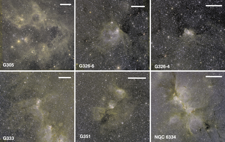
Figure 1. Six star-forming regions observed in our sample. The scale bar in each frame is 5 pc long at the distance given in Table 1. From the upper left to the bottom right: (a) G305 centered at  –
– , (b) G326.6 centered at
  –
– , (c) G326.4 centered at
  –
– , (d) G333 centered at
  –
– , (e) G351 centered at
  –
– , and (f) NGC 6334 centered at
  –
– . In each panel red is the IRAC 4.5 μm long frame time exposure, green is the IRAC 3.6 μm long frame time exposure, and the blue channel is the Ks band image from NEWFIRM.
Download figure:
Standard image High-resolution imageTable 1. Sample 4th Quadrant Massive Star-forming Regions
| Region | R.A. (2000) | Decl. (2000) | Area Observed | Distance |
|---|---|---|---|---|
| (kpc) | ||||
| G305 | 13:11:28.3 | −62:39:46 | 0 47 × 041 47 × 041 |
4a |
| G326-4 | 15:41:46.8 | −53:59:42.9 | 051 × 049 |
2.80b |
| G326-6 | 15:45:06.5 | −54:07:57 | 044 × 045 |
2.68b |
| G333 | 16:21:34.3 | −50:27:04 | 045 × 037 |
3.41b |
| G351 | 17:29:11.2 | −36:43:34 | 045 × 042 |
2.34b |
| NGC 6334 | 17:20:04.0 | −35:53:09 | 09 × 09 |
1.6c |
Notes.
aDistance from Urquhart et al. (2013). bDistances from Bronfman et al. (2000). cDistance from Persi & Tapia (2008).Download table as: ASCIITypeset image
2.1. Spitzer Observations
Data was taken with the Spitzer Space Telescope (Werner et al. 2004) Infrared Array Camera (Fazio et al. 2004) during the warm mission (PID 70157, PI Lori Allen). The dates of observation for each region are given in Table 2. We used IRAC's 12 s frame time High Dynamic Range mode, acquiring consecutive individual observations with exposure times of 0.4 and 10.4 s. The long exposures are used to probe the faint stellar population in each cloud, while the addition of the short exposure observations allows for the recovery of bright sources that are saturated in the long exposure frames. The individual basically calibrated frames (processed with the Spitzer IRAC pipeline version S18.18.0) for each exposure time were mosaicked together using the IRACproc package (Schuster et al. 2006) to perform outlier rejection and bad pixel masking. IRACproc is a PDL4
wrapper script for the standard Spitzer Science Center mosaicing software MOPEX (Makovoz & Khan 2005), which has been enhanced to improve cosmic-ray rejection. Each mosaic was resampled from the native IRAC resolution of 1 22 per pixel to 086267 per pixel, providing pixels with half of the native IRAC size. We projected each mosaic onto a common world coordinate system grid. The final mosaics combined a median of 5 dither positions per pixel for an effective integration time of 52 s per pixel in each long exposure mosaic and 2 s per pixel in each short exposure mosaic. Although all 5 of these star-forming regions were covered by GLIMPSE programs, these new deep data allow us to study the stellar population to 2–3 mag fainter than the GLIMPSE observations.
Table 2. Observation Epochs for 4th Quadrant Star-forming Regions
| Region | IRAC Observations | NEWFIRM Observations |
|---|---|---|
| G305 | 2010 Aug 18 | 2010 May 30 |
| G326-4 | 2010 Sep 15 | 2010 May 30 |
| G326-6 | 2010 Sep 18 | 2010 May 27 |
| G333 | 2011 May 21 | 2010 Jun 01 |
| G351 | 2011 Oct 26 | 2010 May 30 |
| NGC 6334 | 2008 Sep 21 | 2010 May 24, 2010 May 26 |
Download table as: ASCIITypeset image
2.2. NEWFIRM Observations
We also present near-infrared observations of these regions that we acquired with the NOAO Extremely Wide-Field Infrared Imager (NEWFIRM) camera on board the Blanco 4 m telescope at Cerro Tololo Inter-American Observatory during the 2010A semester between 2010 May 24 and 2010 June 1. The NEWFIRM camera, designed to quickly map large areas of the sky, contains 4 InSb 2048 × 2048 pixel arrays arranged in a 2 × 2 pattern with a 28' field of view and an approximately 1' gap between the CCDs. The detector has a pixel scale of 04 per pixel.
Each observation consists of 11 dither positions with 60 s exposures. Our observations were taken with a random dither offset large enough to fill in the 1' gap between CCDs. Each dither position was a combination of multiple co-added exposures to achieve longer exposure times while avoiding the non-linear regime of the detector. For the J band we used two co-added 30 s exposures, for the H band we used three co-added 20 s exposures, and for the Ks band we used six co-added 10 s exposures. The sky background was measured by taking three dithered sky observations 2° off field. The effective exposure time for each band in each star-forming region is 660 s.
Standard processing of dark frame subtraction, flat fielding, sky-subtraction, and bad pixel masking were performed by the NEWFIRM Science Pipeline (Dickinson & Valdes 2009; Swaters et al. 2009) to produce a stacked composite image for each near-infrared band. The final stacked images retain the detector pixel scale of 04 per pixel. Variable seeing conditions caused the final observed point-source FWHM in the stacked images to range from approximately 09 to 15. The difference in effective resolution at the different NEWFIRM bands has a minimal effect on later source-matching.
2.3. Far-infrared Observations
To study the structure of the molecular clouds we also used multiple archival data sets in the far-infrared. The Herschel Infrared Galactic Plane Survey (Hi-GAL) key project (Molinari et al. 2010) observed the Galactic plane between 2010 January and 2012 November. The Hi-GAL program used Herschel's parallel, fast-scanning mode, resulting in simultaneous observation by the Photoconductor Array Camera and Spectrometer (PACS; Poglitsch et al. 2010) and the Spectral and Photometric Imaging Receiver (SPIRE; Griffin et al. 2010) instruments. The data, calibrated according to the Standard Product Generation 9.2.0 were obtained from the Herschel Science Archive.
The observations were recorded in two orthogonal scan directions that were combined into a single map using the Herschel Interactive Processing Environment (HIPE) versions 9.2 and above. Cross-scan combination and de-striping were performed using the standard HIPE tools over the Hi-GAL maps, divided into fields covering 2° × 2°.
Table 3 shows the typical wavelength (in microns) for each band of the Herschel PACS and SPIRE instruments, the angular resolution given by the FWHM of the point-spread function (PSF) calculated by Olmi et al. (2013), and the noise level of the final maps. Position uncertainty of the Hi-GAL maps is of the order of 3'', which is small relative to the PSF at most bands. The noise level given in the table is for SPIRE data taken in "nominal" mode.
Table 3. Summary of Far-infrared Observations
| Instrument | Band | FWHMa | σ |
|---|---|---|---|
| (μm) | ('') | (MJy sr−1) | |
| PACS | 160 | 12.0 | 24.0 |
| SPIRE | 250 | 17.0 | 12.0 |
| SPIRE | 350 | 24.0 | 12.0 |
| SPIRE | 500 | 35.0 | 12.0 |
Note.
aFrom Olmi et al. (2013).Download table as: ASCIITypeset image
Multiple bolometer readings cover each pixel and are combined in the map to determine the observed intensity at each position. Therefore, we can estimate the uncertainty associated with Hi-Gal images from the FWHM of the distribution of the difference between adjacent pixels. In this way, we filter the sky emission that is expected to vary on spatial scales larger than 1 beam-size. The high-pass filter applied to estimate these differences is described in Rank et al. (1999).
The 1σ point-source sensitivities derived from this method are typically 24 mJy for the PACS band at 160 μm, and 12 mJy for each of the three SPIRE bands at 250, 350, and 500 μm. These derived sensitivities are in agreement with those expected for the Hi-GAL survey (Molinari et al. 2010). In addition to the previously derived noise level, we adopt an independent uncertainty of 10% for the flux calibration.
3. SOURCE FINDING AND PHOTOMETRY
We used DAOPHOT (Stetson 1987) to perform PSF-fitting photometry at the J, H, and Ks bands and the long and short exposure mosaics at 3.6 and 4.5 μm for each region. At these wavelengths the level of diffuse nebular emission is relatively low (compared to, for example, IRAC 5.8 and 8.0 μm) so we chose to do only a single iteration for source identification.
The resulting source list was fed into DAOPHOT's ALLSTAR routine to PSF-fit each source. To reduce the effect of crowding, only the flux within a 3 pixel radius was used to fit the model PSF, corresponding to 26 in the IRAC images and 12 in the NEWFIRM images. Detected sources that deviate from the expected point-source shape by more than 5% were rejected. The majority of rejected sources were spurious detections along the extended emission, although we also discard some sources that may be partially resolved background galaxies and pairs of stars with extremely small angular separation.
We used our short exposure images to recover more reliable photometry for bright sources in the IRAC frames. Sources in the long exposure mosaic that matched within 1'' of the position of a short exposure mosaic source with [3.6] < 10 were dropped from the catalog, and the short frame photometry was used instead. A similar cut was used on the 4.5 μm mosaics at [4.5] < 9. Sources that had [3.6] ≥ 10 and [4.5] ≥ 9 adopted a non-linear correction derived from the GLIMPSE point-source catalog. In each band a circular mask was placed around very bright sources to remove spurious detections in the wings of the saturated PSF. The mask size scaled between 2'' and 10'' depending on the brightness of the source.
We used the short exposure mosaic to calibrate the instrumental PSF photometry in each IRAC band against 100 relatively isolated and bright stars measured with aperture photometry in PhotVis (Gutermuth et al. 2004). To determine the zero point for our near-infrared photometry, we matched up bright isolated stars from our NEWFIRM catalogs with sources from the 2MASS (Skrutskie et al. 2006) source list. In the higher source-density portions of the field the 2MASS photometry suffers more from crowding and blending due to the lower survey resolution (24 versus 09), leading to a larger number of sources with artificially bright magnitudes. To decrease the flux contamination effect from this crowding, sources for the near-infrared photometric calibration were carefully chosen from uncrowded portions of the mosaics.
3.1. 4th Quadrant Point-source Catalogs
We created the final source list catalog by spatially matching the detected sources across the five bands. Our cross-band correlation method first calculates whether there is an overall systematic shift in source centroid positions between the input frames and then looks for sources with shifted centroid positions matching between bands. Sources were considered a match if the difference between their shifted centroids was less than than 10.
To further increase the reliability of our point-source catalog, we require simultaneous detection in 2 adjacent bands (e.g., H and Ks on NEWFIRM, or 3.6 and 4.5 μm with IRAC). NEWFIRM sources that are identified only in the Ks band are rejected unless they were detected at both 3.6 and 4.5 μm with IRAC. The completeness limit for each band was determined by recovering fake sources added with DAOPHOT's addstar routine. We created a source list with 5000 fake stars with randomly generated positions, and magnitudes randomly sampled between 8.0 and 18.0 mag for 3.6 and 4.5 μm and between 8.0 and 24.0 mag for the J, H, and Ks bands. We used the derived PSF for each band to add these sources onto the original image and then repeated the original source identification and PSF-fitting steps. We repeated this process 20 times for each photometric band in each region.
We binned the fraction of fake sources that were recovered in bins 0.25 mag wide and took the median fraction of fake sources that were recovered in each bin. The faintest magnitude where the fraction of sources that were recovered was greater than 90% was adopted as the completeness limit. This value varies for each star-forming region and for each band depending on the intrinsic source crowding, the intensity of the nebular emission, and the fraction of the frame that is filled by the nebular emission. The derived completeness limit for each band in each star-forming region is summarized in Table 4. The limiting magnitude reported is the faintest source detected in the original images at the 5σ level or higher (a maximum photometric error of 0.217 mag). A summary of the 4th Quadrant Point-source Catalogs can be found in Table 5. Sample entries selected from the G305.1940 Point-source Catalog can be seen in Table 6 and the full version of the point-source catalog for each region is available in electronic format.
Table 4. Complete and Limiting Magnitudes by Star-forming Region
| Region | Magnitude 90% Complete | Limiting Magnitude | ||||||||
|---|---|---|---|---|---|---|---|---|---|---|
| (J) | (H) | (K) | [3.6] | [4.5] | (J) | (H) | (K) | [3.6] | [4.5] | |
| G305 | 16.0 | 15.1 | 14.7 | 12.8 | 12.5 | 21.8 | 18.9 | 16.9 | 17.4 | 16.6 |
| G326-4 | 16.9 | 16.4 | 14.9 | 13.0 | 13.0 | 21.5 | 19.1 | 17.4 | 17.7 | 16.9 |
| G326-6 | 17.2 | 15.7 | 15.0 | 12.9 | 12.5 | 22.2 | 20.4 | 17.5 | 17.5 | 17.0 |
| G333 | 16.2 | 16.0 | 14.3 | 12.7 | 12.4 | 21.8 | 18.7 | 16.9 | 17.2 | 16.9 |
| G351 | 17.3 | 16.0 | 15.3 | 12.7 | 13.0 | 21.8 | 19.1 | 17.4 | 17.6 | 16.9 |
Download table as: ASCIITypeset image
Table 5. Point-source Catalog Summary
| Region | J Sources | H Sources | Ks Sources | 3.6 μm Sources | 4.5 μm Sources | Four Band Photometrya |
|---|---|---|---|---|---|---|
| G305 | 61256 | 76311 | 44710 | 217878 | 134389 | 34429 |
| G326-4 | 70148 | 86363 | 78248 | 229133 | 146592 | 60980 |
| G326-6 | 79458 | 107340 | 82389 | 233679 | 149920 | 58317 |
| G333 | 58104 | 64713 | 65711 | 220110 | 144883 | 44198 |
| G351 | 70177 | 87429 | 81144 | 223379 | 154177 | 60761 |
Note.
aSources detected at H, Ks, 3.6, and 4.5 μm.Download table as: ASCIITypeset image
Table 6. G305.1940 Point-source Catalog Sample Entries
| R.A. (2000) | Decl. (2000) | J | H | Ks | 3.6 μm | 4.5 μm | Classificationa |
|---|---|---|---|---|---|---|---|
| 13:09:41.990 | −62:53:44.23 | 16.645 ± 0.062 | 15.256 ± 0.016 | −99.0 ± −99.0 | 14.285 ± 0.037 | 14.233 ± 0.045 | 99 |
| 13:09:37.838 | −62:53:41.27 | 17.529 ± 0.079 | −99.0 ± −99.0 | −99.0 ± −99.0 | 16.288 ± 0.104 | −99.0 ± −99.0 | 99 |
| 13:09:54.507 | −62:52:41.17 | 15.067 ± 0.153 | 13.362 ± 0.012 | 12.085 ± 0.012 | 10.25 ± 0.045 | 9.746 ± 0.055 | 2 |
| 13:09:54.507 | −62:52:41.17 | 15.067 ± 0.153 | 13.362 ± 0.012 | 12.085 ± 0.012 | 10.25 ± 0.045 | 9.746 ± 0.055 | 2 |
| 13:12:09.825 | −62:51:10.48 | 15.599 ± 0.119 | 14.397 ± 0.017 | 13.219 ± 0.015 | 11.183 ± 0.083 | 10.071 ± 0.074 | 1 |
| 13:09:46.118 | −62:45:08.68 | 16.421 ± 0.16 | 12.515 ± 0.007 | 10.603 ± 0.119 | 7.11 ± 0.039 | 6.337 ± 0.05 | 1 |
Note.
a1 = Near-infrared-selected Class I YSO, 2 = Near-infrared-selected Class II YSO, 99 = Unclassified Source.Only a portion of this table is shown here to demonstrate its form and content. A machine-readable version of the full table is available.
Download table as: DataTypeset image
4. YSO IDENTIFICATION IN THE 4TH QUADRANT
The Willis et al. (2013) study of NGC 6334 adapted the Spitzer IRAC 4 color criteria to identify YSO candidates that were only detected in the near-infrared and at IRAC's shortest wavelengths 3.6 and 4.5 μm. These selection criteria err on the side of removing more contaminant objects and producing a cleaner sample of YSO candidates, at the expense of rejecting a larger number of real YSOs. As a consequence, the YSO population census derived using these selection criteria will likely miss a fraction of young stars within these star-forming regions that are difficult to disentangle from line-of-sight contaminants.
We applied these YSO selection criteria to our 4th Quadrant star-forming region point-source catalogs. The selection of both Class I and Class II YSO candidates is shown in Figure 2 for G305. The same selection criteria were applied to the other four massive star-forming regions in our 4th Quadrant sample. In total we identified 363 Class I candidates and 2508 Class II candidate YSOs across the five star-forming regions. The number of YSO candidates observed toward each field is given in Table 7.
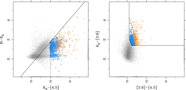
Figure 2. YSO selection cuts applied to the point-source catalog for the region G305, with the log of the field stars distribution shown in the background grayscale. The solid lines mark the boundary of the color–color spaces belonging to YSOs and the dashed lines mark the border between Class I and Class II YSO candidates. The sources selected as Class I YSOs are shown as orange pluses and the sources selected as Class II YSOs are shown as cyan asterisks. The same selection method was used for each of the other star-forming regions (not shown).
Download figure:
Standard image High-resolution imageTable 7. Number of YSO Candidates Identified Using Color Selection Cuts
| Region | Class I | Class II |
|---|---|---|
| G305 | 74 | 769 |
| G326-4 | 48 | 355 |
| G326-6 | 74 | 429 |
| G333 | 113 | 604 |
| G351 | 54 | 351 |
| NGC 6334 | 189 | 1396 |
| Total | 552 | 3904 |
Download table as: ASCIITypeset image
The spatial distributions of the YSO candidate sources throughout each field can be seen in Figures 3 and 4. Viewed in a projection against the cloud, the location of Class I candidates is strongly correlated with the high-density regions that appear as the infrared-dark clouds (IRDCs). The Class II candidates also tend toward a clustered distribution with a larger dispersion than the Class I candidates. Although greater dispersion is expected in the spatial distribution of Class II sources, which are on average older than Class I sources, the larger dispersion also likely indicates that the Class II candidate YSO population is more dominated by contaminant objects, in particular background galaxies.
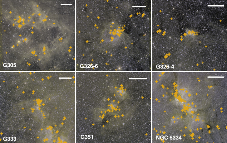
Figure 3. Spatial distribution of all the Class I YSO candidates plotted over the three-color image combining the NEWFIRM and IRAC observations. The scale bar in each frame is 5 pc long. The color mapping and central coordinates are the same as in Figure 1.
Download figure:
Standard image High-resolution image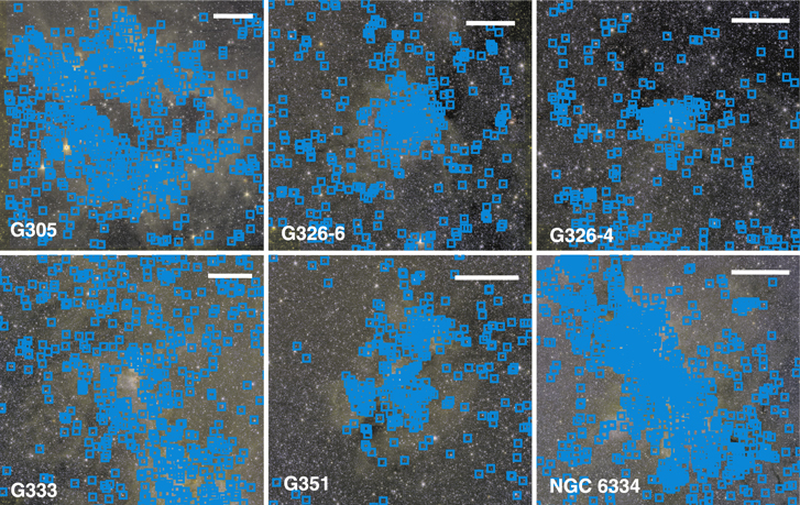
Figure 4. Spatial distribution of all the Class II YSO candidates plotted over the three-color image combining the NEWFIRM and IRAC observations. The scale bar in each frame is 5 pc long. The color mapping and central coordinates are the same as in Figure 1.
Download figure:
Standard image High-resolution image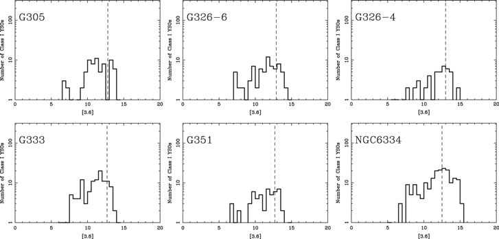
Figure 5. Distribution of 3.6 μm magnitudes for the 363 Class I YSO candidates. The dashed line between 3.6 μm = 12.7 and 3.6 μm = 13 in each panel marks the magnitude corresponding to the 90% completeness limit for the source list derived in each star-forming region.
Download figure:
Standard image High-resolution imageWe show the magnitude histogram for Class I YSOs in Figure 5 and for Class II YSOs in Figure 6. The magnitude histograms of Class II YSO candidates show a larger increase per magnitude bin below the completeness limit than is observed for Class I YSOs, an effect that is most notable for the region G326-4. The effect of this increased contamination is overwhelmed by sources missing due to completeness and sensitivity issues for [3.6] > 14. We provide a brief synopsis of the star-forming properties of each region in the following section. As NGC 6334 was covered in detail in Willis et al. (2013), we refer the reader there for a more complete discussion.
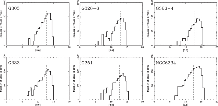
Figure 6. Distribution of 3.6 μm magnitudes for the 2508 Class II YSO candidates. The dashed line between 3.6 μm = 12.7 and 3.6 μm = 13 in each panel marks the magnitude corresponding to the 90% completeness limit for the source list derived in each star-forming region.
Download figure:
Standard image High-resolution image
Figure 7. Column density toward each region measured in magnitudes of equivalent visual extinction. The region G351 shows the column density estimate from a modified near-infrared star counting method, which saturates at AV > 30. The remaining panels show equivalent visual extinctions derived from column density maps produced by fitting modified blackbody curves to Herschel Hi-GAL observations. The scale bar in each frame is 5 pc long.
Download figure:
Standard image High-resolution image4.1. G305
This complex lies at approximately 4 kpc and is one of the most massive (M > 6 × 10⁵ M⊙, Hindson et al. 2010) and luminous (log(Lbol) = 5.94, Urquhart et al. 2013) star-forming regions in the Galaxy (Clark & Porter 2004). The complex displays a ring like morphology of bright mid-infrared emission approximately 30 pc in diameter surrounding two optically visible open clusters Danks 1 & 2 (Davies et al. 2012). The complex contains at least one Wolf–Rayet star but no red supergiants, placing the onset of star formation in the region around 3–5 million years ago (Faimali et al. 2012). Star formation appears to be continuing today in the ring structure surrounding Danks 1 & 2, indicated by results from the Spitzer GLIMPSE program that found an overdensity of young stars with infrared excess distributed along the the nebular emission surrounding the two massive clusters (Indebetouw et al. 2005). Based on the Spitzer GLIMPSE and Herschel Hi-GAL observations of this star-forming complex Faimali et al. (2012) derived a star-formation rate of 0.01–0.02 M⊙ yr−1.
We find that Class II YSOs are widely distributed throughout the outer ring and that the projected area corresponding to the inside of the ring has significantly fewer Class II YSOs. We find that the Class I YSOs are more clustered than the Class II YSOs, with at least six sites indicative of ongoing clustered star formation. We found very few infrared-excess sources that are spatial matches to either Danks 1 or Danks 2, despite their reported youth. Danks 1 is reported to be  Myr based on isochrone fitting to cluster members observed by the Hubble Space Telescope. Danks 2 is reported to be
  Myr based on the same observing program (Davies et al. 2012). Studies of low-mass star-forming regions have determined the average disk half-life is approximately 2 Myr. At 1.5 Myr or even 3 Myr, we should still see a number of infrared-excess sources in these clusters.
The lack of detected sources may be the result of a combination of multiple factors: first, the clusters are very compact and even with PSF-fitting photometry we are unable to resolve many of the individual cluster sources. Second, the majority of the sources in these clusters that are brighter than our detection limit would be intermediate-mass or larger. The pre-main-sequence evolution timescale of stars is expected to be inversely correlated with the star's mass, so the disk dissipation timescale of an intermediate-mass star may be shorter than for low-mass stars. A third possibility is that the close proximity to the large complement of O and B stars may be accelerating the disk dispersal in the few low-mass stars belonging to these clusters that are sufficiently separated to be resolved.
4.2. G326-6 and G326-4
Two of the star-forming regions in our sample lie at approximately l = 326°. The two fields we have observed, which we call G326-4 and G326-6, are centered at l = 326.4, b = 0.9, and l = 326.6, b = 0.5 respectively. These fields contain four bright IRAS point sources (IRAS 15384–5348, IRAS 15394–5358, IRAS 15408–5356, and IRAS 15411– 5352) with kinematic distances from CS(2-1) emission detected by Bronfman et al. (1996) placing them at 2.7–2.8 kpc. Each of the IRAS sources has far-infrared colors that match ultra-compact H ii regions. SIMBA measurements of the 1.2 mm flux estimate that each source contains approximately 103 M⊙ of molecular gas derived from dust continuum observations. The total luminosity of the four IRAS sources is estimated to be log(Lbol) = 5.6 (Faúndez et al. 2004). Observations with the Australian Telescope Compact Array at 4.8 GHz identified a linear feature extending westward from IRAS 15384–5348 that may indicate the presence of an ionized outflow from a protostellar source.
Three of the four IRAS sources lie on the edge of a roughly circular cavity centered at l = 326.675, b = 0.535. The cavity has a radius of r = 4.1', corresponding to approximately 6.4 pc in diameter, assuming a distance of 2.8 kpc. The circular cavity seen in the infrared corresponds to the H ii region RCW 95. A catalog of Spitzer-identified IRDCs identified several dozen sources in this field (Peretto & Fuller 2009). G326-6 hosts the largest H ii region in the field as well as most of the bright IRAS sources including IRAS 15408–5356. Most of G326-4 appears relatively quiescent in the near-infrared images, with extremely bright point sources clustered near IRAS 15394–5358. G326-4 contains both filamentary IRDCs as well as the smaller H ii region associated with IRAS 15384–5348.
The star-forming complexes G326-6 and G326-4 have very small projected spatial separations and distance estimates that are the same to within the typical margin of error (2.68 and 2.8 kpc, respectively). The Bronfman et al. (2000) CS(2-1) catalog lists another source (IRAS 15394–5358) that is spatially located between the major IRAS sources in G326-6 and G326-4, with a velocity that is intermediate between the other two sources. Given the similar distances, small spatial separation, and velocity profile it is possible that the combined G326 field may be one star-forming complex extending at least 60 or more parsecs, with different sub-regions in different evolutionary stages. However, since the Herschel column density maps do not clearly indicate filamentary structures linking the three regions, we treat G326-4 and G326-6 as two separate fields in the subsequent analysis and include IRAS 15394–5358 with the rest of the G326-4 field.
In G326-6 we identified 6 Class I YSO candidates within 0 5 of the far-infrared peak at IRAS 15412–5359. The H ii regions corresponding to the far-infrared sources IRAS 15408–5356 and IRAS 15411–5352 are also detected, with over a dozen YSO candidates each. We have determined a subcluster of YSOs centered at l = 326.672, b = 0.554 containing 13 Class I YSO candidates and 7 Class II YSO candidates within 05. This cluster was not detected by IRAS, indicating that the subcluster does not contain any high-mass stars. Both IRAS 15411–5352 and IRAS 15412–5359 have subclusters of Class II YSOs with small offsets from the peak of the far-infrared emission and the Class I YSO distributions.
G326-4 also has multiple IRAS sources in the field of view, although they are more widely separated than in G326-6 and with no clear indication of connection in the molecular material through filamentary structures. Over half of the YSO candidates in this field were identified toward the extended H ii region corresponding to IRAS source IRAS 15394–5358. Two additional subclusters of Class I YSOs were identified with significant separation from (115 and 112 from IRAS 15394–5358. One of these subclusters, located approximately 115 to the east of IRAS 15394–5358, has no IRAS counterpart. This cluster, located at l = 326.609, b = 0.799 contains 13 Class I YSO candidates. The other YSO cluster is located approximately 112 to the southeast of IRAS 15394–5358, corresponding to IRAS 15394–5358, with the molecular gas at intermediate an velocity between G326-4 and G326-6.
4.3. G333
The star-forming region G333, also known as RCW 106, is another of the most luminous star-forming regions in our galaxy, with log(Lbol) = 6.28 at a distance of 3.6 kpc (Urquhart et al. 2013). The region has a backbone of molecular gas that extends at least 50 pc in a roughly northeast to southwest direction across the star-forming region, with significant diffuse material extending tens of parsecs off of the ridge. Massive star-formation activity is concentrated in pockets along this ridge, as indicated by the presence of compact H ii regions. SIMBA 1.2 mm observations suggest the mass of the giant molecular cloud complex is on the order of 105 M⊙ (Mookerjea et al. 2004). Our observations cover only the central 05 × 04 of this field centered at l = 333.3, b = −0.4. We use the distance estimate 3.45 kpc from (Bronfman et al. 2000) for comparison to earlier works.
Ultimately, our coverage of G333 limits our ability to comment on the global properties of this star-forming region. We have surveyed approximately 50% of the northeastern side of this complex. The Class I YSO population reveals multiple sites of clustered star formation. The two largest clusters of Class I objects correspond to IRAS 16177–5018 and IRAS 16172–5028, compact H ii regions. Both clusters have 19 Class I YSO candidates within 15 of the IRAS source. The widespread population of Class I and Class II YSOs reflects the extent of the nebular emission, suggesting that the extended distributions are due to the physical boundaries of the molecular cloud extending beyond the region observed from the J band to 4.5 μm rather than a high fraction of contamination of background sources.
4.4. G351
The G351 cloud is the second-closest of the clouds in our sample, at a distance of 2.34 kpc. Early observations of G351 resolved the region into two H ii regions using radio recombination line observations at 5 GHz (Caswell 1972), one centered at l = 351.6, b = −1.3 and the other centered at l = 351.7, b = −1.2. Subsequent far-infrared observations using a balloon-borne detector operating at 150 microns, combined with IRAS and detected 7 sources with LIR between 1.1 and 128 × 104 L⊙ (Ghosh et al. 1990). G351.6-1.3 corresponds to an embedded O4 star, while G351.7-1.2 is best fit by multiple sources rather than a single dominating heat source. The other five far-infrared sources Ghosh et al. (1990) that were detected could be heated by either small clusters of B0 or later zero-age main-sequence (ZAMS) stars or a single O6 star. Data from the 2MASS led to the identification of two additional infrared star clusters associated with the nebula (Bica et al. 2003).
The Class I YSOs in this region are primarily found along a northwest to southeast line stretching 20' from IRAS 17256–3631 to IRAS 17258–3637 to the IRDC toward the southeast. Many of these are condensed into two subclusters that appear to be associated with the far-infrared sources and their associated H ii regions. Only two Class I YSO candidates are detected in the IRDC itself. Either this IRDC is quiescent and currently lacks star formation, or the stars that are forming in this IRDC remain too heavily embedded to be detected at H and Ks. The lack of an IRAS source toward this IRDC is an indication that if star formation is active in this cloud, it is primarily forming low-mass stars. Since G351 lacked full Herschel coverage, there is no currently existing data to confirm whether this IRDC has a detectable population of low-mass, embedded protostars, or whether the dark cloud in G351 is not currently active.
4.5. NGC 6334
NGC 6334 and its young stellar content are described in more detail in Willis et al. (2013) and a relatively recent review article by Persi & Tapia (2008). NGC 6334 contains molecular gas on the order of 105 M⊙ and stellar content on the order of 10,000–15,000 M⊙, most of which has formed within the last 2 million years. Several subclusters have age estimates of 1 Myr or less (Getman et al. 2014). NGC 6334 also has a ridge of molecular material extending from the northeast to the southwest, with most of the mass concentrated toward the northeast. There are at least seven H ii regions of various sizes within approximately 10 pc, marking the region as a relatively dense complex of sites of massive star formation. The heavily-concentrated star formation, particularly toward the northeast portion of the cloud, mark NGC 6334 as a potential "mini-starburst" region.
5. DISCUSSION
In this section we use the identified YSO populations and the archival Herschel observations to study the formation of stars as a function of column density within this sample of massive star-forming regions. In particular we examine the existence of a local Schmidt law connecting Σgas with ΣSFR within individual molecular clouds and examine the YSO distributions to determine whether there is a minimum column density threshold for star formation in massive molecular clouds.
5.1. Column Density from Near-infrared Extinction and Herschel Maps
We examine the column density structure of these regions using a combination of maps of the near-infrared extinction and their emission from 160 through 500 μm in the Herschel observations. The star-forming regions we have observed are located at very low Galactic latitudes. As a result, along the line of sight, toward each of these complexes, the majority of point sources observed are unassociated objects, such as background giant stars, background galaxies, and a limited number of foreground objects. The background objects are seen through a high level of extinction, both due to the star-forming regions of interest as well as due to the more diffuse material along the line of sight. Mapping the extinction in the near- and mid-infrared across the region leads to median extinction values of AV ∼ 10 mag. However, many of these clouds contain high-density regions where even at IRAC wavelengths we cannot detect background sources behind the cloud. Toward these dense lines of sight we observe only a small handful of foreground sources. This results in maps that predict extinction values that are too high across the majority of the field where we would expect low to moderate extinction due to the diffuse component of the cloud, and extinction values that are too low toward the dense portions of the cloud that may contain 50% or more of the actual mass.
To reduce the effects of this foreground/background confusion we have used observations from the PACS and SPIRE instruments on board the Herschel Space Telescope to map the column density toward each region. These observations were taken as part of the Hi-GAL guaranteed time program (Molinari et al. 2010) to survey the inner Galactic plane at 70, 160, 250, 350, and 500 μm. The map at each waveband is convolved to the lowest resolution, that of the 500 μm map, using the kernels computed by Aniano et al. (2011). We calculate the median emission in each band within a box size of 30 arcmin in order to produce a map of the diffuse (background) emission, which is subtracted from each waveband. This also eliminates the need to apply an offset correction to the Herschel observations, but decreases the sensitivity of these maps to low column -ensity features that may be associated with the star-forming complexes.
The resulting background subtracted maps were aligned and stacked using MONTAGE.5 The resulting stack has a flux measurement at each pixel for 160, 250, 350, and 500 μm; the 70 μm fluxes are ignored because they are not well fit by a single-temperature modified blackbody. We assume β = 2 and a gas-to-dust ratio of 100. Temperature values below 8 K and column densities below log(NH2) < 20 are unphysical and pixels with these values are ignored in the subsequent analysis.
We extracted column density maps matching the size of the fields for which we had five band coverage (shown in Figure 7) and summed the mass corresponding to the given column densities assuming μ = 2.37. Many of these maps indicate that the structure of these star-forming complexes extend beyond the area for which we have 5 band coverage. In addition, some unknown fraction of the diffuse component that was subtracted from each star-forming region may be diffuse material local to the star-forming region rather than unrelated background/foreground material. For this reason the mass estimates that we utilize here are likely lower limits for the true mass of these complexes, but we restrict our subsequent analysis to the mass densities within the AV > 2 contour for an ease of comparison to Evans et al. (2014) and Padoan et al. (2014).
One region in our sample, G351, is centered around b = 15 and is therefore too far from the Galactic plane to have sufficient coverage in the Hi-GAL survey to generate a column density map. For this region we have generated a map of the density of point sources using our point-source catalog from J band through 4.5 μm. Following the procedure in Cambrésy (1999) we convert the star counts into an estimate of the visual extinction. The star density map provides a more realistic lower-limit of the extinction in high column density areas with AV ∼ 40, although the true column densities may exceed AV > 100. We assume the median level of extinction across the map is due to unrelated line-of-sight material and subtract the median value, AV = 6.9 from the map. We use this background subtracted extinction map in place of the Herschel column density map that we have calculated for each of the other regions. To convert between column density and extinction we adopt N(H2) = 1.37 × 10²¹ AV. The resulting column density maps for each star-forming region are shown in Figure 7.
5.2. The Schmidt Law in Massive Star-forming Regions
We combine the column density information in each region with the spatial distribution of number counts of Class I YSOs. For this analysis, we ignore the Class II population because we assume that the more evolved YSOs are less correlated with the gas structures responsible for their formation. There is some debate whether this offset is due to dynamic motions of the stars within the molecular cloud environment or whether the cloud has moved away from or dissipated in the vicinity of the older stars. Regardless of the origin, as Figures 3 and 4 showed, the spatial extent of the Class II YSOs is broader, and the Class I YSOs are both more clustered and located in closer proximity to the portions of each molecular cloud containing denser gas.
First, we examined the surface density of YSOs (ΣYSO) within different column density contours beginning at AV = 1 and continuing in steps of log(AV) = 0.25. The highest column density contour to examine for each region was determined by requiring a minimum of 2 pixels in the column density map and a minimum of 3 YSOs within the contour. The ΣYSO versus AV is shown in Figure 8.

Figure 8. YSO surface density vs. gas column density in 4th Quadrant star-forming regions. The green points are for G326-6, the blue points are for G326-4, the orange points are for G351, the magenta points are for NGC 6334, the red points are for G333, and the black points are for G305. G326-6 and G326-4 show a vertical offset from the other clouds, which may indicate higher contamination among the detected YSO candidates. NGC 6334 was observed during the cryogenic mission, providing deep 5.8 and 8.0 μm data that enable better detection of YSOs at high column densities.
Download figure:
Standard image High-resolution imageOverall, at low column densities the star-forming regions G326-4 (blue) and G326-6 (green) show the highest YSO surface densities. This may be an indication that these regions have a higher relative fraction of contamination in the YSO sample from objects such as giant stars and background galaxies. However, all of the regions display a relatively low density of YSOs at low column densities, picking up substantially at column densities between AV ∼ 5 and AV ∼ 20. One common result of previous star formation studies has been the determination that AV ∼ 8 is the threshold for star formation (e.g., Heiderman et al. 2010; Lada et al. 2010). Above this critical density star formation is expected to progress according to a Schmidt Law. Below this critical density, star formation will be weak or suppressed.
The extinction is much lower in the infrared than it is at optical wavelengths. Studies of the mid-infrared extinction law find that AK ∼ 0.1AV and A3.6 ∼ 0.6AK (Flaherty et al. 2007). This means that for every magnitude of visual extinction we have about 0.06 magnitudes of extinction at 3.6 μm. So when AV = 15, we are already peering through approximately 1 magnitude of extinction at 3.6 μm. For AV > 40 we may be looking through 3 or more magnitudes of extinction in the near- and mid-infrared. This means that in our magnitude-limited surveys we are likely to miss distinct portions of the YSO population toward both high column density (low surface brightness) regions as well as portions of the observable cloud that are dominated by the bright extended emission excited by the high-mass stars.
We see this effect in Figure 8. The observed surface density of the YSOs reaches a maximum around (or before) AV = 40 in our six massive star-forming regions; above this point we do not detect sufficient numbers of YSOs or sufficiently resolve the column density contours in the majority of our star-forming regions. In NGC 6334, we have a large area with high column density, but we see the surface density of (near-infrared detected) Class I YSOs plummet beyond this peak. For NGC 6334 additional deep observations are available at 5.8 and 8.0 μm that enabled the selection of more embedded YSOs, and even longer wavelength observations from MIPS, Herschel, and the SMA indicate signficant populations of infrared-dark sources at the beginning of the star formation process (e.g., Russeil et al. 2013; Willis et al. 2013; Hunter et al. 2014). However, we use only the near-infrared selected YSOs in the subsequent analysis for direct comparison to the rest of the star-forming regions.
The decrease in YSO density at the higher column densities suggests that we need to account for extinction when we turn our YSO counts (ΣYSO) into a star-formation rate estimate (ΣSFR)—our samples will suffer from incompleteness as we increase to higher column densities. Our method for determining the star-formation rate based on the number of YSOs observed brighter than the magnitude at which the sample is complete includes a correction for the average extinction toward the stars. We used the method described in Willis et al. (2013) to determine the star-formation rate indicated by the YSOs observed at each AV contour by assuming that each star was observed behind an extinction given by the minimum value of that extinction contour. As we increase to higher column densities the total number of stars (both observed and unobserved) decreases, increasing the relative error on these measurements.
In Figure 9 we examine log(ΣSFR) versus log(Σgas) above ∼200 M⊙ pc−2, equivalent to the suggested AV ∼ 8 threshold for star formation (e.g., Heiderman et al. 2010). We fit a linear relation to the data between Σgas ∼ 200 M⊙ pc−2 and Σgas ∼ 3000 M⊙ pc−2, shown as the black dotted line. The red dotted line extrapolates this fit out to higher column densities. We find α = 2.15 ± 0.41 above the assumed critical density AV = 8. The high dispersion reflects the significant differences in the observed star-formation rate within the same minimum column density contour in different molecular clouds. The dashed line shows the extragalactic Kennicutt–Schmidt relation from Kennicutt (1998) for α = 1.4. As we extend our slope determination to lower minimum column densities we find that the fit becomes shallower. The slope for log(ΣYSO) versus log(Σgas) above AV > 2 (Σgas ∼ 50 M⊙ pc−2) is α = 1.59 ± 0.26, and for AV > 1 we find α = 1.37 ± 0.23.
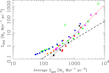
Figure 9. Local Schmidt law in the 4th Quadrant star-forming regions. The green points are for G326-6, the blue points are for G326-4, the orange points are for G351, the magenta points are for NGC 6334, the red points are for G333, and the black points are for G305. The dotted line shows the best fit to the data above the proposed Σgas > 200 M⊙ pc−2 star-formation threshold. The red dotted line extrapolates this relation up to higher gas density. The dashed line shows the extragalactic Kennicutt–Schmidt relation with α = 1.4 (Kennicutt 1998). The green stars mark the reported whole-cloud values for the Galactic mini-starburst regions G035 and W43.
Download figure:
Standard image High-resolution imageThe slope for the power-law behavior above AV > 1 is similar to the alpha = 1.4 slope observed for the galaxy-averaged view of ΣSFR versus Σgas in Kennicutt (1998). However, the slope varies as a function of the column density range examined, flattening as we extend to lower minimum column densities. The variation of the slope as a function of the minimum column density is also consistent with the results from Bigiel et al. (2008), where the slope of the  relation differed depending on the column density regime examined using both atomic and molecular gas. The total gas surface density probed by Bigiel et al. (2008) approximately extends to an order of magnitude below the level we can probe using the Herschel column density maps, which reflects only the presence of molecular gas, not the total HI + H ii gas component of the molecular clouds. Bigiel et al. (2008) found a shallower slope for the power law fit to ΣSFR versus
  at α = 0.96 ± 0.07. Although our data show that the slope becomes shallower at lower column densities, their fits were centered around
  pc−2, which is a factor of 5 lower than the lowest column densities we probe with our maps, and very few of their sub-kiloparsec scale regions contain sufficient dense gas to reach into the Σgas range found in resolved star-forming clouds.
We fit ΣSFR versus Σgas within each molecular cloud individually shown in 10, beginning with the AV > 2 contour and continuing in steps of  to the maximum density in the map. The power-law index for the sample of clouds is between 1.77 < α < 2.86, with the best fit for each cloud given in Table 8. The uncertainty reported for each index is purely based on the G326-4 and G326-6, which we previously identified as appearing to have a higher than expected surface density. YSOs at low column densities also appear to have a slightly shallower slope for ΣSFR versus Σgas below AV ∼ 8, but no significant difference is seen in the power-law slope above AV > 8, compared to AV > 2 for the full sample of clouds. However, the star-formation rates are particularly uncertain toward higher column densities where additional data from longer wavelength observations would assist in recovering the extremely embedded sources.
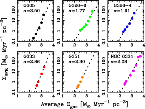
Figure 10. Local Schmidt law in the 4th Quadrant star-forming regions. The dotted lines give the best-fit power law in each region with the spectral index given in Table 8.
Download figure:
Standard image High-resolution imageTable 8. 4th Quadrant Star-formation Rate vs. Gas Density within Individual Clouds
| Region | α |
|---|---|
| G305 | 2.50 ± 0.04 |
| G326.6 | 1.77 ± 0.04 |
| G326.4 | 1.91 ± 0.05 |
| G333 | 2.86 ± 0.03 |
| G351 | 2.30 ± 0.03 |
| NGC 6334 | 2.08 ± 0.08 |
Download table as: ASCIITypeset image
Each individual cloud is well fit by a power law between Σgas and ΣSFR, but the range in star-formation rates seen at the same column density for different clouds increases the scatter in the combined fit to all the star-forming regions. The Herschel column density maps do not provide velocity information that would enable disentangling line-of-sight components at different distances. The clouds in this study are all at very low Galactic latitudes ( ) and potentially signficant levels of foreground or background dust could contribute to the overall difference in star-formation rate at the same column density interval in different clouds. This effect would drive up the scatter when comparing the star formation between different clouds but not significantly affect the slope for the fit to a single cloud.
The average for our sample of molecular clouds finds  once the gas becomes dense enough for star formation to proceed. In Lada et al. (2013), a similar average slope of α = 2.04 ± 0.01 was found for Orion A, Taurus, and California and α = 3.30 ± 0.21 for Orion B. Combined with our sample, these star-forming regions range from extremely quiescent (California Molecular Cloud) to some of the most active star-forming regions in the Galaxy (G305, NGC 6334). The similarity of the power-law indexes indicates that this relation is likely independent of the overall star formation activity of a cloud. We demonstrate this in Figure 11, showing that for both our molecular clouds and the sample of Lada et al. (2013) there is a lack of correlation between the power-law index α and the total luminosity of the cloud at 70 μm, an indicator of the star-formation activity.
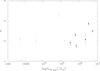
Figure 11. Power-law index α vs. the 70 μm luminosity of the 4th Quadrant star-forming regions (black) and Taurus, California, Orion A, and Orion B molecular clouds from Lada et al. (2013; gray).
Download figure:
Standard image High-resolution imageThis independence is seen both for low-mass clouds that form only a handful of stars, as well as giant molecular clouds that form thousands of stars, including some of the most active GMCs in our galaxy. The relative small spread in the power-law indexes and the lack of correlation between the power-law index and star formation tracers suggests that on the large scale, the process of star formation is occurring in the same manner from low density through high density portions of molecular clouds. Clouds that appear to have a high relative star-formation rate are therefore likely clouds that have a current or recent high fraction of gas sufficiently dense for star formation to progress.
It is interesting to note that the two mini-starburst regions from Motte et al. (2012), W43 and G035, fall more than 2σ above the empirical fit to the 4th Quadrant regions above AV = 8. However, the star-formation rates and gas surface densities for these regions were derived using different methodlogies, so this finding may not be signficant. The 4th Quadrant sample includes clouds with highly concentrated star formation activity, such as the dense ridge that mimics mini-starburst conditions in NGC 6334 (Willis et al. 2013) and the rich young clusters in G305 that have presumably recently formed through mini-starburst-like structure. This result will need to be followed up by combining mid- and far-infrared detected point sources at these high column density ranges to see whether the reported mini-starburst regions show similar behavior to the 4th Quadrant sample. More data will be needed to determine if these apparent differences for the prototypical mini-starburst sources reflect a physical difference in the star formation process in the densest environments.
The star formation history of molecular clouds is not a simple case of either a constant star-formation rate at all times, or an instantaneous burst that immediately forms a large population of stars. Instead, the process of star formation begins and ends, and the total rate and efficiency of the activity vary while it is ongoing. The interplay between the stellar feedback and the diffuse material sculpts the cloud, compressing some gas and dispersing other portions, causing the star-formation rate to vary within a given cloud at a particular time. Both the gas and stars in molecular clouds are in motion, which can potentially lead to an observable offset between dense star-forming gas and young stars over relatively short timescales (Goodman & Arce 2004).
The dissection of galaxies on small spatial scales captures star formation over extended timescales that are much longer than the lifetime traced out by identifying populations of YSOs. The effects of radiative feedback that disperses clouds and the dynamical interactions experienced by young stars that move them relative to the gas are magnified over longer timescales probed by star-formation rate tracers applied in unresolved distant galaxies. This likely contributes to the scatter observed in measurements of the  relation for resolved molecular-cloud sized structures in other galaxies.
Inside molecular cloud complexes in our galaxy we see a tight correlation between the surface density of early-stage YSOs (and their inferred star-formation rate) and gas density inside of a molecular cloud, agreeing with the Schmidt law. Numerous effects, including line-of-sight column density contamination and the relatively small number of observed YSOs contribute to the scatter in observed star-formation rates and gas densities in Milky Way clouds.
It is also important to remember that when we consider a critical density for star formation, we typically use extinction and column density measurements that trace the projected two-dimensional structure of the cloud. In reality, star formation takes place within the three-dimensional gas within the molecular clouds and it is the volume density that should be intrinsically associated with the star-formation activity.
6. CONCLUSIONS
We have presented deep infrared observations of a sample of six massive star-forming regions in the near- and mid-infrared, cataloging ∼200,000 point sources toward each star-forming region. Based on their near- and mid-infrared colors, 2871 of these have been newly identified as 363 Class I and 2508 Class II YSOs, adding to the 375 Class I and 1908 Class II YSOs found in NGC 6334 in an earlier work (Willis et al. 2013). We used Herschel PACS and SPIRE observations from the Hi-GAL program to estimate the column density and in turn the average mass surface density toward five of these molecular clouds. For G351 we used the full point-source catalog to measure the extinction and stellar density across the field.
Our conclusions are as follows.
- 1.This sample of massive star-forming regions is consistent with a general star formation threshold near AV = 8 magnitudes derived from nearby, low-mass star-forming regions.
- 2.Our molecular clouds are well fit by a power law between ΣSFR and Σgas, with the power-law index ranging from 1.77 ± 0.04 to 2.86 ± 0.03.
- 3.The average over the regions sampled indicates
 , similar to nearby primarily low-mass star-forming regions. This indicates that the same physical process are driving the formation of stars in clouds that form low-mass stars and clouds that are capable of forming numerous high-mass stars.
 - 4.Mini-starburst regions (averages) are much higher than the values for the star-forming regions in our sample, even though several of the regions studied contain mini-starburst conditions or have already-formed young starburst clusters.

This work is based on observations made with the Spitzer Space Telescope, which is operated by the Jet Propulsion Laboratory, California Institute of Technology under NASA contract 1407. This research made use of Montage, funded by the National Aeronautics and Space Administration's Earth Science Technology Office, Computation Technologies Project, under cooperative agreement NCC5-626 between NASA and the California Institute of Technology. Montage is maintained by the NASA/IPAC Infrared Science Archive. S.W. acknowledges partial support from NASA grants NNX12AI55G and NNX10AD68G, and JPL-RSA 1369565. S.W. and H.A.S. acknowledge partial support from NASA Grants NNX12Al55G and NNX10AD68G, and JPL-RSA 1369565.