


ABSTRACT
We conduct a series of numerical experiments into the nature of three-dimensional (3D) hydrodynamics in the postbounce stalled-shock phase of core-collapse supernovae using 3D general-relativistic hydrodynamic simulations of a 27 M⊙ progenitor star with a neutrino leakage/heating scheme. We vary the strength of neutrino heating and find three cases of 3D dynamics: (1) neutrino-driven convection, (2) initially neutrino-driven convection and subsequent development of the standing accretion shock instability (SASI), and (3) SASI-dominated evolution. This confirms previous 3D results of Hanke et al. and Couch & Connor. We carry out simulations with resolutions differing by up to a factor of ∼4 and demonstrate that low resolution is artificially favorable for explosion in the 3D convection-dominated case since it decreases the efficiency of energy transport to small scales. Low resolution results in higher radial convective fluxes of energy and enthalpy, more fully buoyant mass, and stronger neutrino heating. In the SASI-dominated case, lower resolution damps SASI oscillations. In the convection-dominated case, a quasi-stationary angular kinetic energy spectrum E(ℓ) develops in the heating layer. Like other 3D studies, we find E(ℓ) ∝ℓ−1 in the "inertial range," while theory and local simulations argue for E(ℓ) ∝ ℓ−5/3. We argue that current 3D simulations do not resolve the inertial range of turbulence and are affected by numerical viscosity up to the energy-containing scale, creating a "bottleneck" that prevents an efficient turbulent cascade.
Export citation and abstract BibTeX RIS
1. INTRODUCTION
Multi-dimensional dynamics is, quite literally, at the heart of core-collapse supernovae from massive stars. Decades of theoretical and computational studies have shown that the hydrodynamic shock formed at the core bounce always stalls and fails to be revived by neutrino energy deposition in simulations that assume spherical symmetry (1D; Bethe 1990; Rampp & Janka 2000; Thompson et al. 2003; Liebendörfer et al. 2005; Sumiyoshi et al. 2005). The advent of detailed axisymmetric (2D) simulations led to the realization that neutrino-driven convection (Burrows et al. 1995; Herant 1995; Janka and Müller 1996) and the advective-acoustic standing accretion shock instability (SASI; Blondin et al. 2003; Foglizzo et al. 2007; Scheck et al. 2008) may both play an important facilitating role in the neutrino mechanism for core-collapse supernova explosions. The nonradial dynamics associated with these instabilities can increase the time material spends in the layer near the stalled shock where net neutrino energy absorption occurs (the "gain layer"). This, in turn, increases the neutrino heating efficiency and creates conditions favorable for launching an explosion (e.g., Murphy & Burrows 2008). Rising convective plumes and large high-entropy bubbles created by SASI-induced secondary shocks can exert mechanical force on the shock and push it out (Burrows et al. 1995; Couch 2013; Dolence et al. 2013; Fernández et al. 2014). As recently pointed out by Murphy et al. (2013) and Couch & Ott (2015), turbulent flow, which is both unavoidable and ubiquitous in the gain layer, provides an effective pressure that adds to the pressure budget behind the shock and thus further helps the multi-dimensional neutrino mechanism.
The set of recent detailed ab initio 2D neutrino radiation-hydrodynamics simulations yields successful explosions in multiple cases and codes (e.g., Marek & Janka 2009; Müller et al. 2012a, 2012b; Bruenn et al. 2013), but failures in others (e.g., Ott et al. 2008; Dolence et al. 2015, who used different approximations for radiation transport and microphysics). One must not rest on the partial 2D success of the neutrino mechanism. Nature is three-dimensional (3D), so are core-collapse supernovae, and so is the multi-dimensional dynamics in their postbounce cores. 3D work was pioneered by the smooth-particle hydrodynamics simulations of Fryer & Warren (2002), but grid-based 3D simulations had to await the broad availability of petascale computing resources and have only recently become possible. Most current 3D simulations do not yet reach the level of their 2D counterparts in implemented and captured physics and in numerical resolution. Yet they are beginning to yield results that elucidate the 3D hydrodynamics of core-collapse supernovae and differences between 2D and 3D (e.g., Burrows et al. 2012; Hanke et al. 2012; Couch 2013; Couch & Ott 2013, 2015; Dolence et al. 2013; Murphy et al. 2013; Ott et al. 2013; Couch & O'Connor 2014; Handy et al. 2014; Takiwaki et al. 2014).
Hanke et al. (2013) and Tamborra et al. (2014) carried out the only 3D studies to date with accurate energy-dependent neutrino transport, which they implement not in 3D, but along many 1D rays. The angular resolution of these simulations is ∼2◦ for both hydrodynamics and neutrinos. Current 3D Cartesian adaptive-mesh-refinement (AMR) simulations with a more approximate neutrino treatment reach much finer effective angular resolutions of 0 4–08 in the gain layer (e.g., Dolence et al. 2013; Ott et al. 2013; Couch & O'Connor 2014).
While there is still much tension between the detailed results (and their interpretation) of current 3D simulations obtained with different approximations and codes, there is consensus that the development of large-scale, high-entropy regions (by neutrino heating or SASI) and, generally, kinetic energy at large scales, is required for a neutrino-driven explosion to succeed (Burrows et al. 2012; Hanke et al. 2012, 2013; Couch & Ott 2013, 2015; Dolence et al. 2013; Murphy et al. 2013; Ott et al. 2013; Couch & O'Connor 2014).
In this work, we systematically study the qualitative and quantitative dependence of 3D postbounce hydrodynamics on the strength of neutrino heating and on numerical resolution. For this, we employ our 3D fully general-relativistic core-collapse supernova simulation code Zelmani introduced in Ott et al. (2012, 2013). This code includes a three-species neutrino leakage scheme, which allows us to control the local efficiency of neutrino heating. We carry out simulations of the postbounce evolution of the 27 M⊙ progenitor model of Woosley et al. (2002), which has been considered by multiple recent studies. Its structure results in a high postbounce accretion rate, which leads to a small radius of the stalled shock, favoring the development of SASI (Müller et al. 2012a; Hanke et al. 2013; Ott et al. 2013; Couch & O'Connor 2014).
We are particularly interested in (i) the prominence of 3D neutrino-driven convection and 3D SASI, their interplay, and their dependence on neutrino heating; (ii) the resolution dependence of postbounce hydrodynamics, neutrino heating, and the development of an explosion; and (iii) the nature of turbulence under neutrino-driven convection-dominated conditions and its dependence on resolution.
We find three general regimes of postbounce 3D hydrodynamics: (1) neutrino-driven convection and the onset of explosion (for strong neutrino heating; e.g., Dolence et al. 2013; Ott et al. 2013; Couch & O'Connor 2014), (2) initially neutrino-driven convection that subsides and is replaced by strong SASI with spiral modes and no explosion (for moderate neutrino heating; consistent with Hanke et al. 2013 and Couch & O'Connor 2014), and (3) complete absence of neutrino-driven convection, SASI-dominated dynamics with spiral modes, and no explosion (for weak neutrino heating). The results of our resolution study show that low numerical resolution artificially damps SASI oscillations in the SASI-dominated case. In the neutrino-driven convection-dominated case, we show that low resolution leads to artificially favorable conditions for explosion. The lower the resolution, the less efficient the cascade of turbulent kinetic energy to small scales (as previously noted by Hanke et al. 2012 on the basis of their simpler "light-bulb" simulations). Low-resolution simulations have higher radial convective kinetic energy and enthalpy fluxes, more buoyant mass in the gain layer, higher neutrino heating rates, larger average shock radii, and transition to explosion earlier than more finely resolved simulations. Analyzing the angular spectra E(ℓ) of turbulence in our simulations, we find a scaling E(ℓ) ∝ ℓ−1 (see Dolence et al. 2013; Couch & O'Connor 2014) at spherical harmonic mode ℓ that should belong to the inertial range of turbulence. By comparison with the literature on local mildly compressible turbulence, we argue that our and other global 3D simulations similar to ours do not resolve the inertial range of neutrino-driven turbulent convection. Instead, numerical viscosity creates a bottleneck that hinders the efficient cascade of turbulent kinetic energy to small scales. Energy is thus kept at large scales, which may, incorrectly and artificially, promote explosion.
We begin in Section 2 with a discussion of our numerical approach and lay out our simulation plan in Section 3. In Section 4, we present results from our simulations in the strong, moderate, and weak neutrino heating regimes and provide detailed analyses of neutrino-driven convection, SASI, and turbulence in these simulations. In Section 5, we present and discuss the results of our extensive resolution study. In Section 6, we put our results into the broader context of the current discussion of the multi-dimensional neutrino mechanism of core-collapse supernovae and conclude.
2. METHODS
We simulate core collapse and postbounce evolution of the nonrotating 27 M⊙ solar-metallicity model of Woosley et al. (2002). We follow collapse, bounce, and the first 20 ms in spherical symmetry using GR1D (O'Connor & Ott 2010) with neutrino leakage and a heating factor fheat = 1.05 (see below for a definition of fheat). At 20 ms after the bounce, the shock has almost stalled. Figure 1 shows the spherically symmetric density, specific entropy, and electron fraction Ye profiles at 20 ms after the bounce. We then map this configuration to our 3D grid and continue the evolution in full 3D. We choose this 1D–3D approach to save computer time during the spherical collapse phase and to avoid having the shock cross the boundaries of the two innermost mesh refinement levels of the 3D grid, which could generate a significant numerical error (Ott et al. 2013). By mapping at ∼20 ms, we miss the earliest part of prompt postbounce convection due to the negative entropy left behind by the weakening shock. Since we are not interested in studying this prompt convection, we believe that our approach is appropriate for the simulations at hand. At the time of mapping, the shock has reached ∼110 km.
The subsequent 3D evolution is performed with the Zelmani core-collapse simulation package (Ott et al. 2012, 2013). It is based on the Cactus Computational Toolkit (Goodale et al. 2003) and it uses modules of the open-source Einstein Toolkit
9
(Löffler et al. 2012; Mösta et al. 2014). We employ a cubed-sphere multi-block AMR system that consists of a set of overlapping curvilinear grid blocks adapted to the overall spherical geometry of the problem (Pollney et al. 2011; Reisswig et al. 2013). The qualitative grid setup is very similar to the one described in Ott et al. (2013) and we refer the reader to their Figure 1 that visualizes the overall structure of our grid. The inner  (along one of the coordinate axes), which contains the protoneutron star and the entire shocked region including the shock, is covered by a cubic Cartesian mesh. This Cartesian region contains four additional co-centric cubic refinement levels. Initially, these levels have radial extents (along the coordinate axes) of (286, 161, 43, 21 ) km. Throughout the 3D simulation, the shock is contained on the third-finest level, whose outer boundary automatically adapts to the shock's position. In our baseline resolution, the grid on the finest AMR level has a linear cell width of 0.354 km. The third-finest level containing the entire postshock region and the shock has a linear cell width of ∼1.416 km. This corresponds to an effective angular resolution of 081 at 100 km and 054 at 150 km.

Figure 1. Density (left ordinate), specific entropy, and electron fraction Ye (both right ordinate) profiles from the GR1D simulation at the time of mapping to 3D, 20 ms after the bounce.
Download figure:
Standard image High-resolution imageThe outer regions are covered by a shell of six angular grid blocks that stretch to 15,000 km. The angular blocks are arranged such that the two angular coordinate directions at each lateral edge of each block always coincide with those from neighboring patches (Reisswig et al. 2013). The angular resolution in those patches is ∼3°, which is sufficient since matter in those regions remains spherically symmetric. The radial resolution at the inner boundary of the angular patches is chosen to be the same as that of the coarsest AMR level, which, for the baseline resolution, is a linear cell width of 5.67 km. The resolution decreases gradually with radius, reaching 189 km at the outer boundary. An important advantange of this multi-block system is that it does not suffer from any coordinate pathologies unlike standard spherical-polar and cylindrical grids.
We solve the 3D general-relativistic hydrodynamics equations in a flux-conservative form (Banyuls et al. 1997) using the finite-volume general-relativistic hydrodynamics code GRHydro (Löffler et al. 2012). It is an improved version of the legacy code Whisky (Baiotti et al. 2005), which itself is largely based on the GR-Astro/MAHC code (Font et al. 2000). We use a customized version of the piecewise-parabolic method (PPM; Colella & Woodward 1984) for the reconstruction of physical states at cell boundaries. The propagation of a quasi-spherical shock on a Cartesian grid creates numerical perturbations that could seed convection at a possibly unphysically high level (Ott et al. 2013; but see, e.g., Couch & Ott 2013). To minimize numerical perturbations, we use the original PPM scheme (Colella & Woodward 1984) on the AMR level that contains the shock. We employ the more aggressive, lower-dissipation enhanced PPM scheme (McCorquodale & Colella 2011; Reisswig et al. 2013) on finer levels, since it outperforms the original PPM scheme in capturing the steep gradients at the edge of the protoneutron star, and, importantly, maintains the smooth physical density maximum at the center of the protoneutron star. The intercell fluxes are calculated via solving approximate Riemann problems with the HLLE solver (Einfeldt 1988).
We evolve the 3 + 1 Einstein equations with the BSSN formulation of numerical relativity (Shibata & Nakamura 1995; Baumgarte & Shapiro 1999). We use a 1 + log slicing (Alcubierre et al. 2000) and a modified Γ-driver (Alcubierre et al. 2003) to evolve the lapse function α and the shift vector βi, respectively. The BSSN equations and the gauge conditions are evolved using the CTGamma code (Pollney et al. 2011; Reisswig et al. 2013).
The hydrodynamics and Einstein equations are evolved in time in a coupled manner using the Method of Lines (Hyman 1976), which uses a multi-rate Runge–Kutta scheme that is second-order in time for hydrodynamics and fourth-order in time for spacetime evolution (Reisswig et al. 2013). We use a Courant–Friedrichs–Levy factor of 0.4 in all of our simulations and the timestep taken on each refinement level is governed by the light travel time along a linear computational cell width.
We employ the tabulated finite-temperature nuclear EOS of Lattimer & Swesty (1991) with  , generated by O'Connor & Ott (2010).10
During collapse, we use the parameterized Ye(ρ) deleptonization scheme of Liebendörfer (2005) with the same parameters as Ott et al. (2013), while in the postbounce phase, we use a three-species (νe,
, generated by O'Connor & Ott (2010).10
During collapse, we use the parameterized Ye(ρ) deleptonization scheme of Liebendörfer (2005) with the same parameters as Ott et al. (2013), while in the postbounce phase, we use a three-species (νe,  ,
,  ) neutrino leakage/heating scheme that approximates deleptonization, cooling, and heating in the gain region (O'Connor & Ott 2010; Ott et al. 2012, 2013; Couch & O'Connor 2014). The scheme first computes the energy-averaged neutrino optical depths along radial rays. Then, local estimates of energy and lepton loss rates are computed. The 3D implementation of this scheme in Zelmani is discussed in detail in Ott et al. (2012, 2013). In contrast to these previous works, we do not include neutrino pressure contributions in this study, since the implementations of the neutrino pressure terms are slightly different in GR1D and Zelmani and tests show that this leads to spurious oscillations of the protoneutron star upon mapping, which, in turn, due to grid perturbations, artificially drives unphysically strong prompt convection upon mapping. Neglecting the neutrino pressure, which contributes ∼10%–20% of the pressure in a narrow density regime from ∼1012.5 to 1014 g cm−3 (Kaplan et al. 2014), results in a slightly more compact protoneutron star, but should not otherwise affect our results.
We approximate the neutrino heating rate  in the gain region by

Here Lνi is the neutrino luminosity emerging from below as predicted by auxiliary leakage calculations along radial rays,  ,
,  , α = 1.23, me is the electron mass, c is the speed of light, ρ is the rest-mass density, mn is the neutron mass, Xi is the neutron (proton) mass fraction for electron neutrinos (antineutrinos),
  is the mean-squared energy of νi neutrinos, and
  is the mean inverse flux factor. fheat is a free parameter, which we refer to as the heating factor. We estimate
  based on the temperature at the neutrinosphere (see O'Connor & Ott 2010) and we parameterize
  as a function of optical depth τνi based on the angle-dependent radiation fields of the neutrino transport calculations of Ott et al. (2008) and set
  . Note that in this parameterization, the flux factor levels off at 1.15 at low optical depth in the outer postshock region. We choose the latter value instead of 1, because the radiation field becomes fully forward peaked only outside the shock (Ott et al. 2008) and because the linear interpolation in
  drops off too quickly compared to full radiation-hydrodynamics simulations. Hence the higher floor value to compensate (O'Connor & Ott 2010). Finally, the factor
  in Equation (1) is used to strongly suppress heating at
  . Further details are given in O'Connor & Ott (2010), Ott et al. (2012), and Ott et al. (2013).
3. SIMULATED MODELS
We carry out a set of eight full 3D simulations, varying the heating factors and numerical resolution as discussed below and summarized in Table 1.
Table 1. Key Simulation Parameters and Results
| Model | fheat | dxshock | dθ, dϕ | tend | Rshock, max | Rshock, avg | Rshock, min | Numerical |
|---|---|---|---|---|---|---|---|---|
| (km) | @100 km | (ms) | @tend | @tend | @tend | Reynolds | ||
| (degrees) | (km) | (km) | (km) | Number | ||||
| s27ULRfheat1.05 | 1.05 | 3.784 | 2.16 | 160 | 295 | 321 | 224 | 53.25 |

|
1.05 | 1.892 | 1.08 | 138 | 248 | 202 | 171 | 62.06 |
| s27MRfheat1.05 | 1.05 | 1.416 | 0.81 | 131 | 233 | 192 | 167 | 68.14 |

|
1.05 | 1.240 | 0.71 | 142 | 229 | 190 | 156 | 70.03 |
| s27HRfheat1.05 | 1.05 | 1.064 | 0.61 | 142 | 215 | 182 | 158 | 72.21 |

|
0.95 | 1.416 | 0.81 | 262 | 79 | 70 | 62 | ... |

|
0.8 | 1.892 | 1.08 | 215 | 82 | 72 | 63 | ... |

|
0.8 | 1.416 | 0.81 | 255 | 85 | 71 | 52 | ... |
Note. fheat is the scaling factor that controls the neutrino heating rate (see Equation (1)); dxshock is the linear cell width on the AMR level that contains the shock; dθ,dϕ @ 100 km is the effective angular resolution at a distance of 100 km from the origin; tend is the time after core bounce when the simulation is terminated; and Rshock, min, Rshock,avg, and Rshock,max are the minimum, average, and maximum shock radii at the end of our simulations, respectively. The procedure for calculating the numerical Reynolds number is discussed in Appendix
Download table as: ASCIITypeset image
We consider strong, moderate, and weak neutrino heating by dialing in heating scale factors fheat = {1. 05, 0.95, 0.8}, expressed in the following model names: s27MRfheat1.05 (strong heating), s27MRfheat0.95 (moderate heating), and s27MRfheat0.8 (weak heating). All of these models have medium numerical resolution, as denoted by "MR" in their model names. This is our baseline resolution discussed in Section 2.
To test for dependence on numerical resolution in the scenario of strong neutrino heating, we take model s27MRfheat1.05 as the reference model and re-run it with four additional resolutions. We characterize these additional simulations by their linear computational cell width on the refinement level that covers the postshock gain layer and contains the shock. Together with our baseline MR ("medium resolution") simulation, we have: ULR (ultra-low resolution, dxshock = 3.784 km), LR (low resolution, dxshock = 1.892 km), MR (medium resolution, dxshock = 1.416 km), IR (intermediate resolution, dxshock = 1.240 km), and HR (high resolution, dxshock = 1.064 km). Note that for the ULR simulation, we have simply taken the LR AMR grid setup and moved the outer boundary of the refinement level covering the shock in the LR simulation down into the cooling layer. In this way, the ULR simulation has the same resolution as the LR simulation in the protoneutron star, but a factor of two lower resolution in the postshock gain layer. All other simulations have systematically changed resolution on all refinement levels.
To test the resolution dependence in the case of weak neutrino heating, we use model s27MRfheat0.8 as the reference model and add one more simulation, model s27LRfheat0.8, with ∼30 % lower resolution than baseline.
4. RESULTS: DEPENDENCE ON NEUTRINO HEATING
4.1. Overview
The top panel of Figure 2 shows the time evolution of the angle-averaged shock radius Rshock,avg in our three baseline-resolution simulations s27MRfheat1.05, s27MRfheat0.95, and s27MRfheat0.8 with strong, medium, and weak neutrino heating, respectively. We show only the part of the evolution tracked in 3D. At early times (t−tbounce ≲ 50–60 ms) the shock undergoes some transient oscillations as it relaxes on the 3D grid, which is reflected in Rshock,avg of all models.

Figure 2. Top panel: average shock radius evolution for models with strong (s27MRfheat1.05), medium (s27MRfheat0.95), and weak (s27MRfheat0.8) neutrino heating. Model s27MRfheat1.05, due to its strong neutrino heating, shows the onset of an explosion already ∼100 ms after bounce. The models with moderate and weak neutrino heating fail to show signs of explosion, but exhibit a transient shock expansion when the accretion rate ( , dashed magenta line) drops at the time the silicon interface accretes through the stalled shock. Center panel: normalized rms deviation σshock of the shock radius from its angle-averaged value. Bottom panel: ratio of the maximum shock radius to the minimum shock radius. Those with moderate and weak neutrino heating exhibit strong periodic oscillations in the shock radius ratio and in σshock. These variations are tell-tale signs of SASI activity in these models.
Download figure:
Standard image High-resolution imageThe average shock radius in model s27MRfheat1.05 grows secularly from  to 125 km in the first 90 ms of postbounce evolution. Subsequently, the shock expansion accelerates and Rshock,avg reaches ∼195 km by ∼130 ms after the bounce, which is when we stop following this model's evolution. The maximum shock radius at this time is ∼220 km. The expansion has become dynamical and is most likely transitioning to explosion. In contrast, models s27MRfheat0.95 and s27MRfheat0.8 do not show any sign of explosion within the simulated time. The average shock radius in these models decreases gradually until ∼160 ms after bounce, reaching ∼97 and ∼75 km, respectively. At this point, the silicon shell reaches the shock front, leading to a sudden decrease of the accretion rate (see the accretion rate shown in the top panel of Figure 2) and thus of the ram pressure experienced by the shock. This leads to a transient expansion of the shock by ∼10 km within ∼15 ms, after which it starts retreating again in both models and continues to do so until the end of our simulations. Due to the weaker heating in model s27MRfheat0.8, Rshock,avg always remains smaller than in model s27MRfheat0.95, but has the same qualitative evolution.
The shock radius evolution shown in Figure 2 can be directly linked to the strength of neutrino heating. We quantify the latter using a set of metrics shown in Figure 3: the integral net neutrino heating rate Qnet, the heating efficiency ( , where
  and
and  are the electron neutrino and anti-electron neutrino luminosities incident from below the inner boundary of the gain region),11
and the mass Mgain in the gain region. The oscillations in these quantities at early times are a combined artifact of the leakage/heating scheme, which is unreliable in highly dynamical situations, and of the shock settling on the 3D grid. Note that the outgoing luminosities are only mildly affected and the main effect comes from variations in the mean neutrino energies; see Ott et al. (2013). Similar features are present in the leakage simulations of Couch & O'Connor (2014). As expected, the larger the fheat (see Equation (1)), the larger the integral net heating, heating efficiency, and the mass in the gain region. Note, however, how strong this relationship is: an increase of fheat from 0.95 to 1.05 (∼10.5%) results in approximately twice as high Qnet, η, and Mgain around 50–100 ms after bounce. This is a consequence of the fact that more intense neutrino heating extends the region of net absorption to smaller radii. It also increases the thermal pressure and the vigor of turblence (and thus the effective turbulent ram pressure; Couch & Ott 2015) throughout this region. This, in turn, pushes the shock out, further increasing the volume of the gain region and leading to more net neutrino energy absorption. This nonlinear feedback shows just how extremely sensitive core-collapse supernovae near the critical line between explosion and no explosion are to the details of neutrino transport and neutrino–matter coupling.
are the electron neutrino and anti-electron neutrino luminosities incident from below the inner boundary of the gain region),11
and the mass Mgain in the gain region. The oscillations in these quantities at early times are a combined artifact of the leakage/heating scheme, which is unreliable in highly dynamical situations, and of the shock settling on the 3D grid. Note that the outgoing luminosities are only mildly affected and the main effect comes from variations in the mean neutrino energies; see Ott et al. (2013). Similar features are present in the leakage simulations of Couch & O'Connor (2014). As expected, the larger the fheat (see Equation (1)), the larger the integral net heating, heating efficiency, and the mass in the gain region. Note, however, how strong this relationship is: an increase of fheat from 0.95 to 1.05 (∼10.5%) results in approximately twice as high Qnet, η, and Mgain around 50–100 ms after bounce. This is a consequence of the fact that more intense neutrino heating extends the region of net absorption to smaller radii. It also increases the thermal pressure and the vigor of turblence (and thus the effective turbulent ram pressure; Couch & Ott 2015) throughout this region. This, in turn, pushes the shock out, further increasing the volume of the gain region and leading to more net neutrino energy absorption. This nonlinear feedback shows just how extremely sensitive core-collapse supernovae near the critical line between explosion and no explosion are to the details of neutrino transport and neutrino–matter coupling.

Figure 3. Integral quantities characterizing the strength of neutrino heating in models s27MRfheat1.05, s27MRfheat0.95, and s27MRfheat0.8 with three different fheat. We also show results for the low-resolution model s27LRfheat0.8.Top panel: integral net neutrino heating rate Qnet (heating minus cooling) in B s−1, where  . Center panel: heating efficiency η defined as Qnet divided by the sum of the νe and
  luminosities emerging from below the inner boundary of the gain region. Bottom panel: mass Mgain (left ordinate) and average specific entropy sgain (right ordinate; not shown for model s27LRfheat0.8) in the gain region. Qnet,η, and Mgain all increase with increasing local heating factor fheat.
Download figure:
Standard image High-resolution imageThe general trends in neutrino heating with fheat described in the above hold throughout the postbounce phase. However, as the shock radii in models s27MRfheat0.95 and s27MRfheat0.8 recede and their gain regions shrink, the values of their neutrino heating variables shown in Figure 3 approach each other. The sudden reduction of the ram pressure at the silicon interface, which has a significant effect on the shock radius (Figure 2), is barely noticeable in the neutrino heating.
We plot the average mass-weighted specific entropy in the gain region (sgain) on the right ordinate of the bottom panel of Figure 3. In agreement with what was found in previous work (e.g., Hanke et al. 2012; Couch 2013; Dolence et al. 2013; Ott et al. 2013), sgain is largely independent of the shock radius and the strength of neutrino heating in the postbounce pre-explosion phase simulated here. We attribute this to two competing effects that affect the averaged quantity sgain: while strong neutrino heating (larger fheat in our simulations) leads to locally higher specific entropy in the region of strongest heating, this is compensated for by the overall larger volume (and mass) of the gain region, which includes material of lower specific entropy that contributes to the average.
After considering the above range of indicative angle-averaged and/or volume-averaged quantities, it is now useful to study deviations from averaged dynamics. The center and bottom panel of Figure 2 depict the normalized rms angular deviation of the shock radius from its mean (Rshock, avg.), σshock, defined as

and the ratio of maximum and mimimum shock radius Rshock,max./Rshock, min., respectively. Both diagnostics yield qualitatively similar results, but the latter is more sensitive to small local variations. In the initial settling phase on the 3D grid, all three simulations shown in Figure 2 exhibit nearly identical shock deviations from sphericity. These are due to moderate-amplitude cubed (ℓ = 4–symmetric) shock oscillations as the models relax from spherical geometry to our 3D Cartesian grid. Subsequently, the shock deviations begin to differ between models. Model s27MRfheat1.05 (strong neutrino heating) shows more or less steadily increasing asphericity as its shock gradually expands and develops large-scale deviations in the maximum shock radius Rshock,max. from Rshock,avg. driven by expanding localized high-entropy bubbles. However, the overall asymmetry, expressed by σshock in Figure 2, is relatively small, due to the strong neutrino heating that leads to a rather global shock expansion.
The shock asphericity in models s27MRfheat0.95 and s27MRfheat0.8 exhibits strong oscillations with clear (if temporally varying) periodicity—a tell-tale sign of active SASI. In model s27MRfheat0.95 (moderate neutrino heating), the oscillations set in around ∼105 ms after the bounce while in model s27MRfheat0.8 (weak neutrino heating), they are already present at ∼80 ms. In both models, the period of the oscillations changes when the silicon interface reaches the shock front around 160 ms after the bounce. We will analyze SASI in these models in more detail in Section 4.2.
Whenever our simulations experience strong neutrino heating, i.e., η ≳ 0.05 and Qheat ≳1052 erg s−1, we find neutrino-driven convection in the postshock region. This is quantified by the top panel of Figure 4, which shows the buoyant mass in the gain region,  , which we define as the mass of material with positive radial velocity.
  correlates strongly with η and Qnet. Phases of strong neutrino heating (see Figure 3) correspond to strong neutrino-driven convection. Model s27MRfheat1.05 undergoes convection throughout its postbounce evolution, while model s27MRfheat0.95 exhibits strong neutrino-driven convection only until ∼110 ms after the bounce. Convective activity is clearly visible in the 2D (x–z plane) entropy color maps of models s27MRfheat1.05 and s27MRfheat0.95 at various postbounce times in Figure 5. We will further analyze neutrino-driven convection in our models in Section 4.3.

Figure 4. Top panel: the mass Mgain,υ > 0 in the gain region with positive radial velocity ("buoyant mass") in models s27MRfheat1.05 (strong neutrino heating), s27MRfheat0.95 (moderate neutrino heating), and s27MRfheat0.8 (weak neutrino heating). Bottom panel: the Foglizzo χ parameter (see Equation (7)) as a function of postbounce time for the three models. The horizontal line at χ = 3 marks the point where convection is expected to develop in the gain region. We calculate χ on the basis of angle-averaged, but not time-averaged, quantities.
Download figure:
Standard image High-resolution image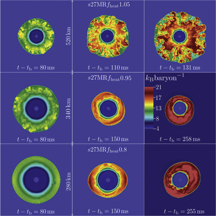
Figure 5. Color maps of specific entropy in the x–z plane in models s27MRfheat1.05 (strong neutrino heating; top row), s27MRfheat0.95 (moderate neutrino heating; center row), and s27MRfheat0.8 (weak neutrino heating; bottom row) at a range of postbounce times. Note that the scale of the region shown is different for each model. Model s27MRfheat1.05 is dominated by neutrino-driven convection. Model s27MRfheat0.95 shows neutrino-driven convection at early times, but subsequently shows signs of coherent shock dynamics typical for SASI. Model s27MRfheat0.8 never develops significant neutrino-driven convection and becomes dominated by SASI.
Download figure:
Standard image High-resolution image4.2. SASI
There are three defining characteristics of SASI: (1) low-(ℓ,m) oscillations of the shock front (e.g., Iwakami et al. 2008), (2) exponential growth of the (spherical harmonics) mode amplitudes in the linear phase (e.g., Blondin et al. 2003), and (3) saturation of the amplitudes once they reach the nonlinear phase (e.g., Guilet et al. 2010). In order to identify these features in our simulations, we decompose the shock front Rshock(θ, ϕ) into spherical harmonics:

where  are the standard real spherical harmonics (e.g., Boyd 2001). We employ the normalization convention used in Burrows et al. (2012), in which a00 corresponds to the average shock radius, while a11, a10, and a1 − 1 correspond to the average x, z, and y Cartesian coordinates of the shock front, respectively.
Figure 6 depicts the normalized mode amplitudes  for
for  (left panels) and ℓ = 2 (right panels) for the three previously introduced models with strong, medium, and weak neutrino heating. The mode amplitudes grow gradually in magnitude over time, which is reflected in the evolution of the angular deviation σ of the shock radius in Figure 2. The relative asphericity of the shock is increasing with time in all models.

Figure 6. Normalized mode amplitudes  of the shock front as a function of time for ℓ = 1 (left panels) and ℓ = 2 modes (right panels). Only modes with m ≥ 0 are shown; modes with negative m behave very similarly. We show amplitudes for models s27MRfheat1.05 (strong neutrino heating, top row), s27MRfheat0.95 (moderate neutrino heating, center row), and s27MRfheat0.8 (weak neutrino heating, bottom row). Note that the range in postbounce time shown in the top row for the exploding model
  is different from the postbounce time covered for the two non-exploding models that develop strong, long-lasting SASI oscillations.
Download figure:
Standard image High-resolution imageIn model s27MRfheat1.05, the ℓ = 1 mode amplitudes grow quickly at 50–80 ms after the bounce, exhibit ∼three periodic modulations with a period of ∼20 ms at nearly saturated magnitude, and then begin to increase to larger values. The ℓ = 2 modes start growing earlier, but show less clear periodicity. The evolution of the ℓ = 1 and ℓ = 2 modes suggest that some form of SASI is present in model s27MRfheat1.05, but a look at the top row of specific entropy slices in Figure 5 reveals that violent neutrino-driven convection is active, fully developed, and driving the local deviation from spherical symmetry at late times in this model.
Models s27MRfheat0.95 and s27MRfheat0.8 exhibit strong SASI oscillations in their ℓ = 1 and ℓ = 2 modes that last for many cycles. The ℓ = 2 modes actually start growing first and the initial growth of all modes exhibits an exponential character until they reach saturation on a timescale of ∼50 ms. The oscillation period is ∼10 and ∼6 ms for ℓ = 1 and ℓ = 2, respectively.
From the x − z specific entropy slices shown in Figure 5, one notes that at ∼80 ms after the bounce there are signs of convection in model s27MRfheat0.95, but no convective plumes are visible in model s27MRfheat0.8 with the weakest neutrino heating. The entropy slices at 150 ms after the bounce show large shock deformations with ℓ = 2 symmetry and no clearly convective features in either model. Interestingly, in both models the ℓ = 2 modes get damped and overtaken by ℓ= 1 oscillations at ∼170 ms after the bounce (see Figure 6), when the silicon interface reaches the shock, leading to transient shock expansion. Accordingly, the late-time entropy slices of these models in Figure 5 exhibit predominantly ℓ = 1 asymmetry.
Although the accretion of the silicon interface damps the initially dominant ℓ = 2 modes significantly (see Figure 6), they again, but only episodically, reach large amplitudes at later postbounce times. This is uncharacteristic of linear growth of physical models and may possibly be due to nonlinear interactions with the then-dominant ℓ = 1 modes.
The ℓ = 1, m = {−1, 0, 1} modes shown in Figure 6 have different phases with respect to each other. This is suggestive of "spiral" SASI oscillations as identified, e.g., by Blondin & Mezzacappa (2007), Fernández (2010), and Iwakami et al. (2014). We analyze the vector

which gives the direction and magnitude of the ℓ = 1 shock deformation with respect to the center of the protoneutron star (Hanke et al. 2013). We visualize the time evolution of  with a line in 3D space in the top and bottom panels of Figure 7 for models s27MRfheat0.95 and s27MRfheat0.8, respectively. Each point on the graph is color coded according to postbounce time t − tbounce. During the early postbounce evolution,
  is small and does not exhibit any clear rotational patterns in either of the models. After the silicon interface has accreted through the shock, the ℓ = 1 modes reach large amplitudes. It is then (orange–red colors in Figure 7) that
  clearly describes several complete spiral cycles in both models. This confirms the spiral nature of the late ℓ = 1 SASI, which is qualitatively very similar to what Hanke et al. (2013) and Couch & O'Connor (2014) found in their 3D simulations of the same progenitor.
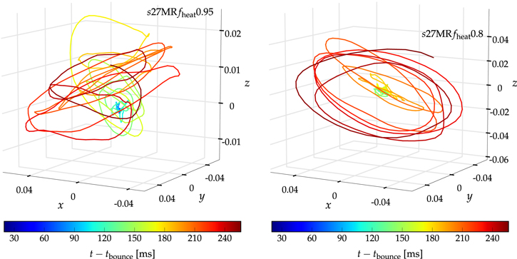
Figure 7. Evolution of the normalized ℓ = 1 mode vector  for models s27MRfheat0.95 (top panel) and
  (bottom panel). The viewing directions on each panel are chosen to be perpendicular to the plane of the spiral SASI motion when it reaches the largest amplitude. The color of the graphs demarks time. Both models exhibit spiral SASI oscillations, but they are strongest in the model with weakest neutrino heating, s27MRfheat0.8.
Download figure:
Standard image High-resolution imageIt is interesting to ask why we observe an early growth of the ℓ= 2 SASI mode in our simulations while ℓ = 1 is usually identified to be the most unstable SASI mode. We speculate, fueled by T. Foglizzo (2015, private communication), that one possible explanation may be related to the trend found by Foglizzo et al. (2007) that higher values of ℓ are favored when the shock radius is small. Just before the accretion of the silicon shell interface, the average shock radius Rshock,avg in models s27MRfheat0.95 and s27MRfheat0.8 is as small as 97 and 75 km, respectively. The reduction in ram pressure at the silicon interface lets the shock jump outward, possibly creating a situation more favorable for ℓ = 1 oscillations than before. This might be the reason for the sudden damping of the ℓ = 2 modes and the development of the ℓ = 1 oscillations.
In the simulations of the same 27 M⊙ progenitor of Ott et al. (2013), Couch & O'Connor (2014), and Hanke et al. (2013), the ℓ = 1 modes reach large amplitudes before the accretion of the silicon interface. It dominates over ℓ = 2 at least in the early evolution in Couch & O'Connor (2014) and Ott et al. (2013; Hanke et al. 2013 do not provide ℓ = 2 amplitudes). In these simulations, the average shock radius is nearly always above 100 km in the early postbounce phase. It drops below this value early on in our present simulations with weak (s27MRfheat0.8) and moderate (s27MRfheat0.95) neutrino heating. Following the above argument, this may explain why only our simulations exhibit an initially predominantly ℓ = 2 SASI.
It is worth mentioning that, to the best of our knowledge, strong excitation of predominantly ℓ = 2 modes in the 3D case was observed only in the work of Takiwaki et al. (2012), who studied the 3D postbounce hydrodynamics in a 11.2 M⊙ progenitor. However, in their simulation, this mode undergoes only 2–3 oscillations during the simulated time, whereas in our case, we observe ∼30 oscillation cycles before ℓ = 2-dominated dynamics ceases. The ℓ = 2 modes also reach large amplitudes in the 3D simulations of Iwakami et al. (2008), Ott et al. (2013), and Couch & O'Connor (2014), but their amplitudes generally do not exceed those of the ℓ = 1 modes.
4.3. Neutrino-driven Convection
Neutrino heating in the gain region establishes a negative radial entropy gradient (e.g., Herant et al. 1992) and thus can drive convection. In stable stars, convection occurs on a stationary background. Not so in the postshock region of a core-collapse supernova: material accreting through the stalled shock is advecting toward the protoneutron star with velocities up to a few percent of the speed of light. In order for convection to fully develop, convective plumes must not only be buoyant with respect to the rest frame of the background flow, but must be able to rise in the laboratory (coordinate) frame against the background advection stream.
Depending on the accretion rate (determined by the progenitor structure; e.g., O'Connor & Ott 2011), strength of neutrino heating (i.e., steepness of the entropy gradient), and initial size of the perturbations entering through the shock from which buoyant plumes can grow, one can identify three different regimes of convection: (1) dominance of advection, where plumes do not even become buoyant in the rest frame of the accretion flow; (2) plumes are buoyant in the rest frame of the accretion flow, but are still advected out of the gain region into the convectively stable cooling layer; (3) plumes are fully buoyant and rise against the accretion flow. As we shall see, our simulations cover all three of these regimes.
We analyze buoyant convection in our simulations with the Ledoux criterion (Ledoux 1947) and express its compositional dependence in terms of the lepton fraction Yl:

where  is the sum of entropies of the matter s and neutrino field
  , while
  is the lepton fraction. Since our leakage/heating scheme does not track the neutrino distribution function, we set Yl = Ye and
  in Equation (5). This is a very good approximation in the gain region, where neutrinos are almost free streaming, but is less accurate in the protoneutron star where neutrinos are trapped at densities above
  . A fluid parcel is convectively stable if
  and unstable otherwise. In the latter case, the linear growth time of small perturbations to buoyant plumes is given, approximately, by the inverse of the Brunt–Väisälä (BV) frequency,

so  implies instability. Here, g is the local free-fall acceleration, which we approximate as
  in our postprocessing analysis, where M(r) is the mass enclosed within radius r. A similar approach was used in, e.g., Buras et al. (2006b), Takiwaki et al. (2012), and Ott et al. (2013).
In addition, we compute the Foglizzo χ parameter (Foglizzo et al. 2006),

where  is the radial velocity in the gain region. χ can be interpreted as the ratio of the advection timescale to an average timescale of convective growth. Any small linear seed perturbation (coming, e.g., from turbulent convection in nuclear burning shells; e.g., Arnett & Meakin 2011; Couch & Ott 2013, 2015) accreting through the shock can at most grow by a factor of
  during its advection through the gain region. For such linear-scale perturbations, Foglizzo et al. (2006) found that
  is necessary for convection to develop in the gain region. The situation is different for large seed perturbations for which the time integral of buoyant acceleration is comparable to the advection velocity (Scheck et al. 2008). In this case, a seed perturbation may develop into a buoyant plume and stay in the gain region instead of being advected out. The results of Scheck et al. (2008) suggest that seed perturbations of
  may be sufficient to allow fully developed convection even when
  . Fernández et al. (2014) pointed out that χ is quite sensitive to the way it is calculated. We follow the recent works of Ott et al. (2013), Couch & O'Connor (2014), and Hanke et al. (2013), who all used instantaneous angle-averaged quantities to compute χ via Equation (7).
If convection develops (either in regime 2 or 3, which we introduced earlier in this section), its vigor can be measured using the anisotropic velocity  defined as (Takiwaki et al. 2012)

where  denotes an angular average at a fixed radius r.
  measures the magnitude of the velocity component that is not associated with a purely spherically symmetric radial background flow.
  is high in regions of large angular variations in
  and large nonradial velocities
  and
and  .
.
Convective activity in our simulations can be diagnosed via Figure 4 (showing the amount of buoyant mass and Foglizzo χ), Figure 5 (showing color maps of 2D  entropy slices at various postbounce times), and Figure 8 (showing the evolution of radial profiles of the angle-averaged BV frequency
  and
and  ).
).

Figure 8. Color maps showing radial slices of the angle-averaged Brunt–Väisälä (BV) frequency ωBV (Equation (6); left panels) and anisotropic velocity υaniso (Equation (8); right panels) in models s27MRfheat1.05 (top panels), s27MRfheat0.95 (center panels), and s27MRfheat0.8 (bottom panels). Also shown are the maximum (red curves), the average (blue curves), and the minimum (green curves) shock radii. We do not show ωBV and υaniso outside the minimum shock radius. Note the differing temporal and radial scales chosen for different models.
Download figure:
Standard image High-resolution imageIn all models, within milliseconds of the bounce, a convectively unstable region with a steep negative entropy gradient develops inside the radial shell ranging from  to
to  due to the propagation of the gradually weakening shock. In our simulations, this phase occurs already during the 1D evolution with GR1D (not shown here). This leads to the development of strong prompt convection within
  after the start of the 3D simulations, as is evident from the
  profiles shown in Figure 8. The χ parameter (Figure 4) is generally
  in all models, but prompt convection develops nevertheless from numerical perturbations, which are
  at the time the profile is mapped from one dimension to three dimensions and settles on the 3D grid (see the discussion in Ott et al. 2013 about perturbations from the Cartesian computational grid). Prompt convection smoothes out the negative entropy gradient on a timescale of 5–10 ms, leading to a rapid weakening and then to complete disappearance of convection. The latter is most apparent from the dramatic decrease in buoyant mass shown in the top panel of Figure 4.
Deleptonization at the edge of the protoneutron star creates a negative lepton gradient within 30–40 km. It drives convection in the protoneutron star, setting in at 35–50 ms after the bounce (Figure 8). Protoneutron star convection (albeit modeled only schematically, given the limitations of our neutrino treatment; see Section 2) is similar in all models, since it is independent of neutrino heating in the gain region.
In model  , neutrino heating creates a negative entropy gradient in the region between
  and the shock, leading to a convectively unstable layer, as apparent from the upper left panel of Figure 8. This triggers and sustains convection in the postshock region starting at
  , at this early time aided by additional entropy perturbations coming from variations in the shock radius. The amount of buoyant mass (top panel of Figure 4) has a local maximum when convection first starts and exceeds this maximum only once the explosion begins to develop in model
  . The Foglizzo χ parameter shown (bottom panel of Figure 4) suggests that much of the convection, while clearly visible in the entropy slices of this model shown in Figure 5, is not fully bouyant in the coordinate frame (regime 2). Only at
  after the bounce does χ grow beyond the linear-theory threshold value of 3 and the amount of buoyant mass increases, indicating that convection is now fully buoyant and convective plumes begin to push out the stalled shock, driving both its expansion and asymmetry (regime 3). These general trends agree well with what was found by Burrows et al. (2012), Couch (2013), Dolence et al. (2013), Ott et al. (2013), and Couch & O'Connor (2014) for 3D simulations with strong neutrino heating that yielded explosions.
In model  with moderate neutrino heating, the buoyant mass peaks when neutrino-driven convection first develops and then gradually declines with time. While we see clear signs of convection in the entropy snapshot at
  after the bounce in Figure 5, convective plumes never become fully buoyant in the coordinate frame in this model, and regime 3 of fully developed buoyant convection is never reached. At
  after the bounce, convection has all but disappeared and the buoyant mass has plummeted. At this point, SASI has taken over from neutrino-driven convection as the dominant hydrodynamical instability (see Section 4.2). It is the driving agent for the large anisotropic motions visible at late times in Figure 8.
Finally, in model  with weak neutrino heating, convective instability is weak and only intermittent. As in the other models, the amount of buoyant mass peaks at
  after the bounce, but convection weakens quickly and is almost gone at
  after the bounce, as is obvious from the entropy snapshot of this model shown in Figure 5. SASI dominates the postbounce hydrodynamics in this model and is responsible for the strong anisotropic dynamics diagnosed via
  in Figure 8 at later postbounce times.
4.4. Turbulence
Turbulence has recently become the center of attention in core-collapse supernova theory and simulation (Murphy & Meakin 2011; Murphy et al. 2013; Couch & Ott 2015). In the absence of very rapid core rotation and strong magnetic fields (the most likely scenario for the vast majority of massive stars; Heger et al. 2005; Ott et al. 2006), there is no physical source of viscosity in the postshock gain layer that could prevent neutrino-driven convection from developing into high Reynolds number turbulence (see Appendix
A growing number of core-collapse supernova studies analyzing turbulence are showing that one of the key differences between 2D and 3D simulations is the well known (e.g., Kraichnan 1967) inverse and unphysical 2D turbulent cascade that drives kinetic energy toward large scales in 2D instead of toward small scales in three dimensions (e.g., Hanke et al. 2012; Couch 2013; Dolence et al. 2013; Takiwaki et al. 2014; Couch & O'Connor 2014; Couch & Ott 2015). Simulations suggest that kinetic energy at large scales is favorable for explosion, which may explain why 2D simulations appear to explode more easily than 3D simulations in many studies. Moreover, work by Murphy et al. (2013) and Couch & Ott (2015) demonstrated that the effective pressure generated by turbulent stress in the postshock region is an important contribution to the overall pressure behind the shock and likely pivotal in launching an explosion against the preshock ram pressure of accretion.
Turbulence in the postshock region of core-collapse supernovae is anisotropic in the radial direction and quasi-isotropic in nonradial motions (Murphy & Meakin 2011; Murphy et al. 2013; Handy et al. 2014; Couch & Ott 2015). It is mildly compressible (reaching pre-explosion Mach numbers of ∼0.3–0.5; Couch & Ott 2013) and only quasi-stationary. In the following, we focus on the kinetic energy spectra of turbulence in our simulations and compare neutrino-driven convection-dominated and SASI-dominated regimes of postbounce hydrodynamics.
We study the spectrum of turbulent motion in our simulations by decomposing the kinetic energy density of the nonradial motion into spherical harmonics on a spherical shell in the gain layer. Following previous work by Hanke et al. (2012), Couch (2013), Dolence et al. (2013), Couch & O'Connor (2014), and Handy et al. (2014), we define coefficients

where  and where we average the
  part within the radial shell
  . In our analysis, we use
  ,
,  , where
  is the minimum shock radius at the time we carry out the spatial averaging (we also tested variations of R1 and R2, i.e., (0.7–0.9)
 and
and  and found no significant difference in the spectra). The total angular kinetic energy density at a given ℓ is then

In order to calculate  at time t, we additionally average
  over the time interval
  , where we take
  in our analysis. We note that in the literature it is more common to express the turbulent energy spectrum in terms of the wave number k instead of ℓ. However, since we are decomposing the nonradial motion on a spherical shell, spherical harmonics are the natural choice. We expect
  to be a power law
  , with α varying between different ranges in ℓ. Any power-law spectrum
  corresponds to
  in the limit of large ℓ (e.g., Chapter 21 of Peebles 1993) and, as pointed out by Hanke et al. (2012), the power-law indices of
  and E(k) should correspond well to each other already at
  .
.
Studies of 3D turbulent flows in various scenarios have shown that the spectrum of turbulent motion  consists of three different regions (e.g., Pope 2000). The energy of the turbulent flow is supplied in the energy-containing range at large spatial scales comparable to the size of the turbulent region by creating large-scale turbulent eddies with ℓ ~ a few. In the energy-containing range,
  is typically nearly constant or increases mildly with ℓ. The inertial range is the range in ℓ in which energy cascades (i.e., is transferred) from large-scale eddies down to small scales and
  decreases with
  . In the dissipation range, the dependence of
  on ℓ is significantly steeper than in the inertial range, typically
  (e.g., Pope 2000). Our simulations do not contain any physical viscosity (which would, in any case, be extremely small in the postshock gain layer; see Appendix
In the Kolmogorov theory of isotropic, incompressible, stationary turbulence (e.g., Landau & Lifshitz 1959),  in the inertial range. For the case of neutrino-driven convection in the gain layer, we expect a similar or even steeper scaling, since (1) turbulence is more or less isotropic in the nonradial directions considered here (Murphy et al. 2013), (2) turbulence has sufficient time to fully develop, since the pre-explosion stalled-shock phase lasts for many turnover cycles, and (3) a higher Mach-number (more compressible) flow generally leads to a more efficient turbulent cascade to small scales, and thus a steeper power law (e.g., Garnier et al. 2000).
The top panel of Figure 9 shows  at various postbounce times in model
  , whose gain-layer hydrodynamics is dominated by neutrino-driven convection due to strong neutrino heating (see Section 4.3). While there are variations in
  in the low-ℓenergy-containing range, at
  the spectra are quite steady after
  , indicating that the flow is at least quasi-stationary at intermediate and small scales in this model.
  should peak at ℓ, corresponding to the size of the convectively unstable gain region. At
  after the bounce we infer from the top right panel of Figure 8(a) the radial extent of the turbulent region of
  and a typical radius of
  (the center of the convective region). The value of ℓ at which the spectrum
  peaks should correspond to the number of eddies with diameter H that fit into the turbulent region,
  . This is close to what is realized by the spectrum at
  after the bounce shown in Figure 9 for this model. At smaller scales (larger ℓ), the spectrum should first exhibit an extended inertial range region with
  before steepening in the dissipation range at very large ℓ. This, however, is not borne out by Figure 9. At intermediate ℓ of 10–40, the spectrum is much shallower than
  and most consistent with ℓ−1, and it steepens only at
  and quickly surpasses the
  scaling. This kind of spectral behavior is qualitatively and quantitatively consistent with what was found for neutrino-driven turbulence in the simulations of Dolence et al. (2013), Couch & O'Connor (2014), and Couch & Ott (2015), who all used numerical methods and Cartesian grid setups very similar to ours.

Figure 9. Top panel: angular spectra  of the angular kinetic energy density of convective turbulent motion (Equation 10) in model
  at a range of postbounce times before the onset of shock expansion. We overplot lines indicating
  (Kolmogorov) and ℓ−1 scaling. The energy-containing range is near
  and should be linked by the inertial range to the dissipation scale at large ℓ.
  is most consistent with ℓ−1 scaling in the "inertial range," which suggests that numerical viscosity affects the efficiency of kinetic energy from large to small scales. Bottom panel: angular spectra
  for model
  (weak neutrino heating) at various postbounce times. In this SASI-dominated model, turbulence is driven by shear and entropy gradients associated with secondary shocks. The
  spectrum is highly nonstationary at all ℓ.
Download figure:
Standard image High-resolution imageThe bottom panel of Figure 9 shows  at various postbounce times in the SASI-dominated model
  (weak neutrino heating). Anisotropic motions in this model (and at postbounce times
  also in model
  whose
whose  is not shown) are driven by entropy and vorticity perturbations caused by the SASI, which is much more intermittent than neutrino heating. This is reflected in the turbulent kinetic energy spectra that vary at all scales with postbounce time and do not reach the quasi-stationarity that we observe for neutrino-driven turbulent convection in the top panel of Figure 9. The variations in
  in the SASI-dominated model can be directly correlated with the strength of SASI. For example, the overall magnitude of
  grows from 90 to 150 ms after the bounce, which coincides with the increasing strength of SASI oscillations seen in Figure 6 for this model. At
  ,
,  at large scales is decreased as a result of damped SASI oscillations shortly after the silicon interface advects through the shock (see Section 4.2). While there is much variation in the overall magnitude of
  , the scaling of
  is significantly shallower than
  and closer toℓ−1 at the scales one would naively be tempted to identify with the inertial range. This is in agreement with the neutrino-driven turbulent convection case.
Several authors (e.g., Dolence et al. 2013; Couch & O'Connor 2014) have argued that the ℓ−1 scaling observed in contemporary 3D simulations could be due to the physical nature of the postshock turbulent flow that deviates significantly from the assumptions of Kolmogorov turbulence. Our interpretation is different. An inertial range scaling with  with
with  is unphysical, since in the limit of infinite resolution, the integral turbulent energy is divergent. Neutrino-driven turbulence is essentially isotropic in the nonradial directions, is quasi-stationary, and is only mildly compressible. Local high-resolution studies of driven turbulence in this regime generally find an inertial range with
  for the incompressible transverse flow component and
  for the compressible part (e.g., Schmidt et al. 2006). Those simulations and simulations of turbulence in other regimes (e.g., Porter et al. 1998; Sytine et al. 2000; Dobler et al. 2003; Kaneda et al. 2003; Haugen & Brandenburg 2004; Kritsuk et al. 2007; Federrath 2013), however, also find the appearance of a shallower region with
  near the end of the inertial range before the transition to the dissipation range. This corresponds to inefficient energy transport at these scales and is referred to as the bottleneck effect. This is understood to be a physical feature of turbulence that is related to a partial suppression of nonlinear interactions of turbulent eddies of different scale near the regime of strongest dissipation (She & Jackson 1993; Yakhot & Zakharov 1993; Falkovich 1994; Verma & Donzis 2007; Frisch et al. 2008).
Sytine et al. (2000) carried out a resolution study with local compressible (Mach 0.5) freely decaying turbulence simulations using the original PPM solver of Colella & Woodward (1984). Their Figure 11 shows that their local simulations with 10243 and 5123 cells resolve an inertial range with  . The bottleneck with
  appears at the end of this range. However, with decreasing resolution, the bottleneck shifts to progressively lower wavenumbers, consuming more and more of the resolved inertial range. Already at 2563, the inertial range is gone and energy injection and dissipation scales are joined directly with
  . On the basis of their results and previous work by Porter et al. (1998), Sytine et al. (2000) argue that the numerical viscosity of their PPM scheme provides dissipation that directly affects the flow on spatial scales from 2 to ∼12 times the width of a computational cell. This should be the equivalent of the dissipation range. On somewhat larger scales, from ∼12 to ∼32 cell widths, the flow is still indirectly affected by the viscosity of PPM, creating the observed bottleneck effect. We point out that these studies focused on a specific regime of turbulence, freely decaying and isotropic, which is different from the one we observe in our simulations. In our simulations, turbulence is driven by buoyancy and is anisotropic. However, very recently, Radice et al. (2015) came to conclusions very similar to Sytine et al. (2000) also for driven anisotropic turbulence.
Our numerical hydrodynamics scheme is very similar to the PPM implementation used by Sytine et al. (2000), but likely more dissipative because we do not employ the original exact Riemann solver of Colella & Woodward (1984), but the more dissipative HLLE solver (see Section 2). The numerical viscosity of our scheme is thus larger than in the scheme of Sytine et al. (2000; see the comparison between HLLE and HLLC in Radice et al. 2015), and 32 cell widths is only a lower bound on the scale, which is affected by numerical viscosity in our simulations. In our fiducial medium resolution simulations for which we present  in Figure 9, the cell width is
  and the region that is turbulent has a radial extent of
  (see Figure 8). Hence, we have (in the best case) 70 km/1.4 km ≈ 50 cells covering the turbulent region (of which ∼32 are affected by numerical viscosity), which is much less than the 512 linear cell width needed by Sytine et al. (2000) to resolve an inertial range. We conclude that at the resolution employed here, we cannot reasonably expect to resolve the inertial range in the turbulent gain layer. All that we are seeing here, and that the simulations of Dolence et al. (2013), Couch & O'Connor (2014), and Couch & Ott (2015) show, is the contamination of the turbulent energy spectrum by numerical viscous effects all the way up to the energy-containing range. Turbulence is thus not resolved in these and in the present 3D simulations. This conclusion is further supported by the low numerical Reynolds number of
  that we find in Appendix
  via a simple comparison of the size of the convective region with linear grid spacing (e.g., Pope 2000). Using their approach, we find
  . Authors carrying out simulations on spherical grids have argued that they see α closer to
  and resolve the inertial range (Hanke et al. 2012; Handy et al. 2014). However, the angular and radial resolutions employed in these studies are significantly lower than the effective resolutions provided by our 3D Cartesian grids, and it is not clear how the turbulence could be resolved in their simulations if not in ours.
5. RESULTS: DEPENDENCE ON NUMERICAL RESOLUTION
5.1. Strong Neutrino Heating, Convection-dominated Regime
We explore the impact of numerical resolution in the regime of strong neutrino heating and neutrino-driven convection-dominated 3D hydrodynamics by running simulations of the s27 progenitor with a total of five different resolutions with the linear cell width in the postshock gain layer varying by almost a factor of four. Our baseline  model has a resolution on the AMR level containing the postshock region and the shock with linear resolution
  . This correponds to an effective angular resolution at a radius of
  of
of  . In models
  ("ultra-low resolution"),
  ("low resolution"),
  ("intermediate resolution"), and
  ("high resolution"), this is
  ,
,  ,
,  , and
, and  , respectively. These correspond to effective angular resolutions at a radius of
  of
of  ,
,  ,
,  ,
,  , and
, and  , for ULR, LR, IR, and HR, respectively (see also Table 1).
Figures 10 and 11 give a concise summary of the effects of resolution on the postbounce hydrodynamics and on the development of a neutrino-driven explosion. The overall trend is very clear: the lower the resolution, the larger the average shock radius, the higher the neutrino heating rate, the greater the heating efficiency, and the larger the mass in the gain layer.
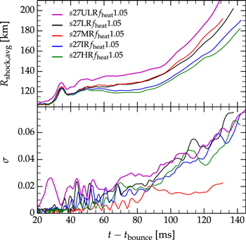
Figure 10. Top panel: evolution of the average shock radii for five different resolutions in the strong neutrino heating regime ( ; see Table 1 for simulation details). Lower resolution leads to larger shock radii. Bottom panel: Evolution of the normalized rms deviation
  of the shock radius from its angle-averaged value for the same five models.
Download figure:
Standard image High-resolution image
Figure 11. Time evolution of the integral net neutrino heating Qnet (top panel), heating efficiency η (center panel), mass in the gain region Mgain (bottom panel, left ordinate), and the average entropy in the gain region sgain (bottom panel, right ordinate) for the case of strong neutrino heating and five different resolutions. Low resolution results in artificially efficient neutrino heating and in an overestimate of the mass in the gain region.
Download figure:
Standard image High-resolution imageWhile these overall trends are robust, there are some notable inconsistencies in the details. The mean specific entropy in the gain layer (bottom panel of Figure 11) appears almost completely independent of resolution. The asphericity of the shock front, measured by the normalized rms deviation  of the shock radius in the bottom panel of Figure 10 has no systematic resolution dependence in its magnitude and variations. The fiducial MR simulation is an outlier with the overall smallest
  . The shock radius, neutrino heating, heating efficiency, and mass in the gain region are very similar in the LR and MR models (differing in dxshock by ∼30%), and at the end of its evolution the MR simulation actually has a slightly larger shock radius than its LR counterpart. On the other hand, the IR and HR simulations, which differ only by
  in resolution, are consistent with each other in all quantities except
  . The MR/IR simulation pair differs in resolution by
  , yet their results are much farther apart than those of the LR/MR pair that differs by
  in resolution. These variations from the general trend are indicative of the possibility that many if not most (or all) of our simulations are not yet in the convergent regime. Perhaps much higher resolutions in the convectively unstable layer may be needed to accurately and in a converged manner capture the hydrodynamics of core-collapse supernovae dominated by neutrino-driven turbulent convection.
Hanke et al. (2012), Couch & O'Connor (2014), and Takiwaki et al. (2014), who carried out less extensive 3D parameter studies with similar or lower resolutions, found the same trends with resolution observed in our simulations. Handy et al. (2014), on the other hand, found improved conditions for explosion with increasing resolution. However, they studied angular grid spacings from 24° down to only 2°. Their highest resolution roughly corresponds to our ULR case. At such coarse resolutions, which suppress nonradial convective motions, it is not at all surprising that the conditions become more favorable for explosion as increasing resolution begins to allow nonradial motions. The Handy et al. (2014) simulations thus probe the resolution dependence of 3D postbounce hydrodynamics in a completely different regime than our simulations.
Figure 12 provides further evidence for why lower-resolution simulations are (artificially) favorable for neutrino-driven explosions. The lower the resolution, the larger the amount of buoyant mass (defined as the mass in the gain region with positive radial velocity) and the greater the amount of positive momentum in the gain region. The more mass is truly buoyant (and thus in regime 3 of neutrino-driven convection discussed in Section 4.3), the greater the neutrino heating rate and efficiency (see Figure 11). Note, however, that by comparing the total mass in the gain region given in the bottom panel of Figure 11 with the buoyant mass in the top panel of Figure 12, one finds that that the truly buoyant mass is at most  of the mass in the gain region. We expect that this fraction will sensitively depend on progenitor structure and will be higher in progenitors with lower postbounce accretion rates than in the 27
  progenitor that we study here.
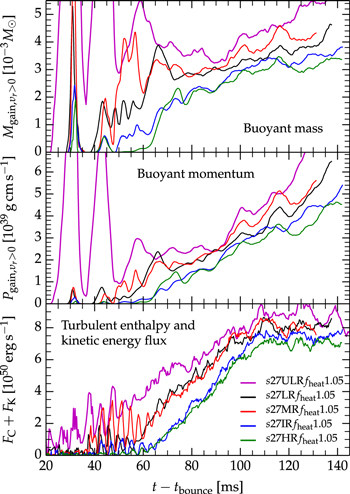
Figure 12. Comparison of buoyant mass (top panel), buoyant momentum (center panel), and radial convective enthalpy and kinetic energy fluxes (bottom panel; see Equation (11)) for simulations with five different resolutions of the strong neutrino heating case. Higher-resolution simulations, in particular in the first  after the bounce (before shock expansion sets in), have smaller
  ,
,  , and
, and  than lower-resolution simulations.
Download figure:
Standard image High-resolution imageThe bottom panel of Figure 12 shows the time evolution of the sum of the angle-averaged "turbulent" radial fluxes of enthalpy (FC, also known as "convective flux") and kinetic energy (FK) near the shock. We follow Hurlburt et al. (1986) and Handy et al. (2014) and define
where ρ is the density,  is the radial velocity,
  is the internal energy, P is the pressure, and
  is the ith component of velocity. All primed quantities represent variations about the angle-averaged mean so that, for instance, FK measures the amount of the turbulent part of the specific kinetic energy (note that by construction
  , where
  denotes the angular average). We evaluate the angular integrals in Equation (11) at each time at a radius that corresponds to the instantaneous minimum shock radius. A number of studies (e.g., Burrows et al. 1995; Couch 2013; Dolence et al. 2013; Ott et al. 2013; Handy et al. 2014; Couch & Ott 2015) have argued that buoyant convective/turbulent bubbles are locally important in driving shock deformation and expansion. Murphy et al. (2013) and Couch & Ott (2015) have shown that the additional effective ram pressure due to turbulence is crucial for the relative ease of explosions in two dimensions and three dimensions compared with the 1D case. All these effects are related to the convective/turbulent flux of kinetic energy and enthalphy in the gain layer and near the shock (see Yamasaki & Yamada 2006). Figure 12 reveals that the sum
  near the shock decreases with increasing resolution, creating less favorable conditions for explosion.
The radial convective/turbulent fluxes are dominated by the flow at large and intermediate scales. In Figure 13, we plot angular turbulent kinetic energy spectra  (see Equation (10)) in the gain layer at
  after the bounce for all resolutions. The left panel shows the plain
  spectra, while the right panel shows "compensated" spectra that are rescaled by
  as is customary in studies of Kolmogorov turbulence. A flat graph in the region where the inertial range is expected would indicate consistency with Kolmogorov turbulence. Given the spatial scale of the gain layer in our simulations, we would expect the energy-containing range to be around
  (see Section 4.4), which should be followed by an inertial range with
  before dissipation sets in. None of our simulations, not even the HR case, exhibits any inertial range. Where the inertial range should be,
  is most consistent with an ℓ−1 scaling, which is indicative of a bottleneck due to viscous contamination because of insufficient numerical resolution (see Section 4.4).
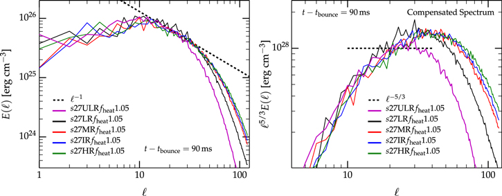
Figure 13. Left panel: angular spectra of the turbulent kinetic energy density for five different resolutions at  after the bounce in the strong neutrino heating case. The turbulent transport of energy to small scales becomes increasingly efficient with increasing resolution. Decreasing resolution leads to an onset of strong dissipation at smaller ℓ. Right panel: compensated (
 rescaled) turbulent spectra. The dashed line indicates the range in ℓ where we expect the inertial range and where the spectrum should be flat if
  were realized as predicted by theory.
Download figure:
Standard image High-resolution imageFigure 13 does not clearly show large differences of  in the energy-containing range with changing resolution. However, note that at low ℓ the spectra are not fully stationary (see Figure 9). One should also recall that we here project out the radial part and that the important radial kinetic energy and enthalpy fluxes decrease with increasing resolution, which indicates less total energy/power at large scales (Figure 12). The figure does, however, clearly demonstrate that transport of turbulent energy to small scales becomes increasingly efficient as the resolution is increased. The energy contained at large ℓ increases systematically with resolution and even appears to converge as the resolution gets close to the HR case. However, the resolution decrements between the various shown simulations are not constant and the three highest simulations differ only by
  in resolution, while MR and LR differ by
  and LR and ULR differ by a factor of two. Since no inertial range is realized, we do not consider any of our studied resolutions to be in the regime in which the flow is truly turbulent. The HR simulation, at
  after the bounce, covers the entire postshock region with
  computational cells, but only the outer
  are actually convectively unstable and are effectively covered by
  linear cell widths. According to Sytine et al. (2000) this resolution may still be a factor of ≳7–8 too low for resolving the inertial range.
5.2. Weak Neutrino Heating, SASI-dominated Regime
We investigate the resolution dependence in the weak neutrino heating, SASI-dominated case by comparing our baseline-resolution simulation  with a simulation carried out with lower resolution,
  , which uses the same resolution of the LR simulation as in the previous section. MR and LR resolutions differ by
  (see Table 1). Additional simulations with further decreased or increased resolution would be advisable but were not possible for the SASI-dominated case within the limitations of our computational resources.
The top panel of Figure 14 compares the evolution of the average shock radius in the MR and LR simulations. They are qualitatively and quantitatively nearly identical and significantly closer to each other than the LR and MR simulations in the strong neutrino heating case discussed in the previous Section 5.1. We also find (and show in Figure 3) that integral net neutrino heating, neutrino heating efficiency, and the mass in the gain region are very similar in the MR and LR models throughout the simulated postbounce time.

Figure 14. Top panel: comparison of the average shock radius evolution in the MR and LR simulations of the SASI-dominated  model with weak neutrino heating. The MR and LR resolutions differ by
  . The shock radius evolution is almost independent of resolution in this model and until
  after the bounce. Then, the shock in the higher-resolution (MR) simulations expands somewhat, possibly related to the appearance of large-scale
  SASI modes at this time (see Figure 15). Bottom panel: the normalized rms deviation
  of the shock radius from its angle-averaged value in the MR and LR simulations. The oscillations in
  , which are due to SASI, are much stronger in the MR simulation, indicating that SASI is weaker in the LR simulation (see Figure 15).
Download figure:
Standard image High-resolution image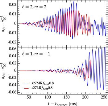
Figure 15. Comparison of select normalized mode amplitudes  of the shock front between the LR and MR simulations of the SASI-dominated
  model. The top panel shows the
  mode and the bottom panel shows the
  mode. The qualitative evolution of the modes are nearly independent of resolution and behave as discussed in Section 4.2 for this model. However, the magnitude of the mode amplitudes is generally lower in the lower-resolution simulation. The resolutions differ by
  .
.
Download figure:
Standard image High-resolution imageWhile the average shock radius evolves nearly identically in the MR and LR cases, we find that deviations from the average due to SASI oscillations are smaller in the LR case. This is apparent from the bottom panel of Figure 14, which shows the normalized rms deviation  of the shock radius from its angle-averaged value. The oscillations in
  are due to SASI, and their amplitudes are much smaller in the LR simulation. Figure 15 depicts the evolution of the normalized
  and
and  amplitudes (Equation (3)) of the shock front as representative examples of the
  mode families in the LR and MR simulations. The evolution of these modes is qualitatively similar in both LR and MR simulations, but the LR simulation shows systematically lower mode amplitudes in both
  and
and  until
until  after the bounce. At that time, the silicon interface advects through the shock, leading to its transient expansion, and to a profound change in the SASI mode structure (see Section 4.2). In the LR simulation, the
  mode amplitudes decay less than in the MR case, but the
  modes do not grow as strongly as in the MR case. This deviation between MR and LR SASI dynamics has an effect on the average shock radius, whose MR and LR evolutions depart from each other toward the end of the LR simulation at
  after the bounce.
Our results show that the weak neutrino heating, SASI-dominated regime of 3D postbounce hydrodynamics is sensitive to resolution and this sensitivity is strongest in the development and nonlinear dynamics of SASI. Sato et al. (2009) have shown that for SASI to reach convergence, the numerical resolution must be sufficiently high to capture the full advective-acoustic cycle of entropy/vorticity perturbations that advect through the postshock region, are reflected at the protoneutron star, and propagate back up to the shock. The LR simulation ( ) has evidently too low resolution, but since we only have two resolutions at hand, we cannot with confidence say that the MR simulation (
 ) is in the convergent regime for SASI.
6. DISCUSSION AND CONCLUSIONS
Core-collapse supernovae are fundamentally 3D. The 3D simulations presented in this paper add to the growing set of modern 3D simulations that are beginning to elucidate the many facets of postbounce hydrodynamics in neutrino-driven core-collapse supernovae. Our results—in agreement with Hanke et al. (2013) and Couch & O'Connor (2014)—show, beyond a reasonable doubt, that 3D postbounce hydrodynamics can be dominated by neutrino-driven convection or by the SASI, or can involve both at the same time or at different times.
SASI is not an artifact of axisymmetry (2D), but is, at least in current 3D results, generally associated with high postbounce accretion rates, with moderate or weak neutrino heating, and with failed 3D explosions in progenitors that explode in two dimensions (Burrows et al. 2012; Hanke et al. 2013; Ott et al. 2013; Couch & O'Connor 2014). An interesting open question is now if 3D SASI-dominated core-collapse supernovae can still yield explosions or if their progenitors are part of the possibly large fraction of massive stars that simply do not explode and result in black holes (Kochanek 2014, 2015; Clausen et al. 2015). Hanke et al. (2013) found an explosion in at least one SASI-dominated case of a 25  progenitor, but that simulation used an artificial contracting inner boundary, dialed-in inner boundary neutrino luminosity, and a gray neutrino transport scheme. Their more sophisticated energy-dependent radiation-hydrodynamics 3D simulation of the same 27
  progenitor studied here shows SASI-dominated dynamics and does not appear to yield an explosion.
There is broad consensus now that high (kinetic) energy at scales comparable to the size of the postshock gain layer is favorable for shock expansion and explosion. More (buoyant) nonradially moving mass in the gain layer increases the efficiency of neutrino heating (e.g., Buras et al. 2006a; Murphy & Burrows 2008). Large-scale convective radial fluxes of buoyant material, associated with buoyant high-entropy bubbles (due to neutrino-driven convection or SASI) can deliver heat and do mechanical work on the shock (Burrows et al. 1995; Yamasaki & Yamada 2006; Hanke et al. 2012; Couch 2013; Dolence et al. 2013; Ott et al. 2013; Couch & O'Connor 2014; Handy et al. 2014). The effective pressure of turbulence at large scales adds to the thermal pressure in the postshock region and facilitates larger shock radii, and thus helps the explosion (Murphy et al. 2013; Couch & Ott 2015).
If it is indeed energy/power/dynamics at large scales that is needed to revive the stalled shock, then the results of our resolution and turbulence study in this paper do not at all bode well for the standard neutrino mechanism in 3D. We studied effective angular resolutions in the postshock gain layer from  (which is the resolution used in Hanke et al. 2013 and the highest resolution considered by Handy et al. 2014) to
  . Going from the lowest to the highest resolution, the neutrino heating rate drops precipitously (by
  ), and so do the total amount of mass in the gain layer, the amount of buoyant mass, and the convective fluxes of kinetic energy and enthalpy. The result is a smaller average shock radius and a slower transition to explosion with increasing resolution. Our model with strong neutrino heating still shows at least the onset of an explosion even in the highest resolution, but in a more critical case, a low-resolution simulation may incorrectly predict an explosion where a higher-resolution simulation does not.
Our results, in agreement with the results of the simpler "light-bulb" simulations carried out by Hanke et al. (2012), show that the higher the resolution in 3D, the more efficient becomes the turbulent cascade of nonradial kinetic energy to small scales. Moreover, comparing our results for the turbulent energy spectra with what is expected from turbulence theory and local simulations of mildly compressible turbulence, we find that even our highest-resolution simulation does not resolve the inertial range of turbulence. Instead, the realization of turbulence in our simulations is likely affected by numerical viscosity all the way up to the scale of energy injection. This reduces the efficiency of the turbulent cascade to small scales and results in a shallow scaling of the angular energy spectrum. The same is likely true also for the simulations of Dolence et al. (2013) and Couch & O'Connor (2014), who find similarly shallow scalings.
In our highest-resolution simulation, the turbulent gain layer is covered by ∼66 linear computational cell widths. Sytine et al. (2000) argue that the numerical viscosity of the PPM scheme affects regions of up to ∼32 cell widths and that  linear cell widths across a mildly compressible turbulent region are necessary to resolve any inertial range with PPM. This would, in the best case, correspond to ∼7–8 times our current resolution in the gain layer. Should our conclusion be correct, then obtaining neutrino-driven explosions will just get harder when higher-resolution simulations become available that resolve the inertial range and efficiently transport energy to small scales. The standard neutrino mechanism may then need help to somehow corral energy at large scales and/or a source of additional heating. For example, large-scale perturbations from pre-collapse aspherical shell burning were shown by Couch & Ott (2013) to boost the vigor of turbulence and thus could help. Magnetic fields could help converge the flow to long-lived high-entropy bubbles (Obergaulinger et al. 2014), and the dissipation of Alfvén waves propagating from a magnetized protoneutron star into the gain layer may be an additional source of heat (Suzuki et al. 2008). Moderate rotation in combination with the magnetorotational instability could also lead to additional heat input into the gain layer (Thompson et al. 2005).
Work in the immediate future will need to be directed toward better understanding turbulence in the core-collapse supernova context. This can be addressed first with local simulations that adopt flow conditions characteristic of the gain layer and resolve a significant inertial range. Such simulations should be able to test the conclusions we have drawn on the basis of our global simulations. Subsequently, high-resolution semi-global simulations could be used to test the ramifications of not resolving the inertial range.
We thank Sean Couch, Peter Goldreich, and Mike Norman for helpful discussions on turbulence and Thierry Foglizzo for help with interpreting the behavior of SASI in our simulations. We furthermore acknowledge helpful discussions with Adam Burrows, Joshua Dolence, Steve Drasco, Rodrigo Fernandez, Sarah Gossan, Thomas Janka, Bernhard Müller, Jeremiah Murphy, Evan O'Connor, Sherwood Richers, and other members of our Simulating eXtreme Spacetimes (SXS) collaboration (http://www.black-holes.org). This research is partially supported by NSF grant Nos. AST-1212170, PHY-1404569, PHY-1151197, PHY-1212460, and OCI-0905046, by NSERC grant RGPIN 418680-2012, by a grant from the Institute of Geophysics, Planetary Physics, and Signatures at Los Alamos National Laboratory, by the Sloan Research Foundation, and by the Sherman Fairchild Foundation. C.R. and L.R. acknowledge support by NASA through Einstein Postdoctoral Fellowship grant Numbers PF2-130099 and PF3-140114, respectively, awarded by the Chandra X-ray center, which is operated by the Smithsonian Astrophysical Observatory for NASA under contract NAS8-03060. The simulations were performed on the Caltech compute cluster "Zwicky" (NSF MRI award No. PHY-0960291), on supercomputers of the NSF XSEDE network under computer time allocation TG-PHY100033, on the NSF/NCSA Blue Waters system under NSF PRAC award ACI-1440083, on machines of the Louisiana Optical Network Initiative, and at the National Energy Research Scientific Computing Center (NERSC), which is supported by the Office of Science of the US Department of Energy under contract DE-AC02-05CH11231. The multi-dimensional visualizations were generated with the open-source VisIt visualization package (https://wci.llnl.gov/codes/visit/). All other figures were generated with the Python-based matplotlib package (Hunter 2007, http://matplotlib.org/).
APPENDIX A: DISSIPATION OF TURBULENT MOTION
The parameter used to indicate the onset of turbulence is the physical Reynolds number,

where ℓ is a length scale of the flow, u is a velocity scale of the flow, and ν is the physical kinematic viscosity. Laboratory experiments show that the transition from laminar to turbulent float occurs at  , depending on the geometry of the experimental boundaries (see Arnett et al. 2014).
The kinematic viscosity is related to the efficiency of momentum transport by particles in the fluid. Employing the Chapman-Enskog procedure to first order on the Boltzmann equation gives the kinematic viscosity

where  is the transport cross section for particles in the fluid (see Mekjian 2013). Therefore, particles that have the smallest total cross section but large average momentum (i.e., electrons are unlikely to contribute) will be responsible for the viscosity in the medium. Clearly, neutrons will have the smallest interaction cross section due to their neutrality. Therefore, the kinematic viscosity in the postshock region is given by Mekjian (2013; assuming the thermal DeBroglie wavelength is greater than the neutron s-wave scattering length
  ),
),

The convectively unstable gain layer has a typical length scale of  and typical velocities of
  . Hence, for
  and
and  , we obtain an estimate for the physical Reynolds number of

which is larger than what would be predicted just using the Braginskii-Spitzer viscosity (Braginskii 1958; Spitzer 1962) and clearly implies the system should be turbulent.
Momentum exchange due to neutrino emission, absorption, and scattering has also been invoked as a source of viscosity that can damp turbulent convection in core-collapse supernovae and protoneutron stars. The neutrino viscosity in the opaque and semi-transparent regimes was estimated by, e.g., Burrows & Lattimer (1988), Keil et al. (1996), and Thompson & Duncan (1993). Here we provide an estimate of the relevance of neutrino viscosity in the gain region, where neutrinos stream relatively freely.
The specific momentum deposition rate due to neutrino absorption in the gain region can be estimated as

where  is the electron neutrino luminosity emerging from the neutrinosphere, nuclei are assumed to be dissociated, neutrino–nucleon interactions from Burrows et al. (2006) are employed (electron scattering is neglected),
  is the characteristic neutrino cross section scale defined in Burrows et al. (2006), and the luminosity in all neutrino flavors is assumed to be equal. Since most of these neutrinos propagate in the radial direction, momentum will mostly be deposited in that direction. This will not dampen stochastic turbulent flow, for which momentum needs to be exchanged between turbulent eddies. However,
  can still be used as an upper limit for momentum exchange between different turbulent eddies. Using (16), one can estimate the timescale for momentum change in the gain region due to
  :
:
where P is the characteristic momentum of the largest turbulent eddies in the gain region and  is their characteristic velocity. The latter is roughly equal to
  (Equation (8)). The timescale of convective motion of eddies of size λ in the gain region can be estimated as

For  , which is a reasonable estimate for the eddy scale, we get
  , implying that momentum exchange due to neutrinos is unimportant at large scales. At smaller scales, the characteristic turbulent eddy velocity is given by (e.g., Pope 2000)
where  is the size of the largest eddies. Combining (16) and (18), we get
  . The characteristic timescale of turbulent eddies scales with λ as (e.g., Pope 2000)

i.e.,  decreases with λ faster than
  does, hence
  remains much larger than
  for any λ. In other words, momentum exchange due to neutrinos cannot damp turbulence in the gain region.
APPENDIX B: EFFECTIVE REYNOLDS NUMBER
Our simulations do not include any explicit physical viscosity but rely on the viscosity of the numerical scheme to model the unresolved scales of the turbulent cascade, in accordance with the implicit large eddy simulation (ILES) paradigm (Garnier et al. 2000). The ILES procedure has been shown to be robust and accurate for a number of turbulent flows as long as the effective Reynolds number, defined as

with  being the "numerical viscosity", is sufficiently large, e.g., Zhou et al. (2014). That is, as long as there is a sufficient separation between the energy-containing scale l0 and the dissipation scale lD. How large the scale separation should be in order for the ILES procedure to reach convergence (in a statistical sense), is problem-dependent. Nevertheless, it is useful to measure the range of scales covered by our simulations in a quantitative way. This will also ease the comparison with future simulations.
Unfortunately, estimating the effective Reynolds number in ILES calculations is not trivial because the numerical viscosity does not really behave like a physical viscosity, that is, it cannot easily be associated with a given kinematic viscosity coefficient  . Instead, it is a complex nonlinear function of the hydrodynamic quantities. Nevertheless, in the framework of Kolmogorov's theory of turbulence, it is possible to construct measures of the Reynolds number that do not explicitly depend on
  . In particular, our estimate of the Reynolds number is based on the Taylor length (e.g., Pope 2000):

where Z is the enstrophy

and E is the total energy

In the incompressible limit, the average kinetic energy dissipation rate is related to the enstrophy via the relation

where ν is the kinematic viscosity. Furthermore, in Kolmogorov's theory of turbulence the energy dissipation rate is assumed to be

where C is of the order of one (here assumed to be C = 1) and l0 is the integral scale, i.e., the scale of energy-containing eddies. Substituting (24), (25), and (23) into (21) and using the definition of the Reynolds number, we obtain

We compute the enstrophy in our numerical data as

where  is the radius at which the spectra are computed and we restrict our calculation to
  , because, for ℓ ≳ 120, the floating point precision necessary to compute the associated Legendre functions can exceed the limits of the double precision employed in our analysis code. In computing (27), we used the fact that the k2 factor in the Fourier expansion corresponds to (minus) the Laplacian in the physical space and that, by definition,

so that a k2 factor in the Fourier expansion corresponds to a  factor in the angular expansion.
E is computed in a similar way to Z, summing the angular expansion coefficients of the energy (Equation (10)) up to ℓ= 120. From the values of Z and E, we can infer  for model
  at
at  after the bounce. The Taylor length is sometimes interpreted as being the radius of the smallest coherent structures of the turbulent flow, so it is not surprising that we find λ to be roughly 13 cells, close to the scale at which we expect numerical dissipation to be too strong for coherent structures to persist.
The integral scale is computed as

where we compute ℓ0 via

We find, for model  ,
,  corresponding to
  . The corresponding Reynolds number is
  .
.
As a sanity check, we can use another identity for  (Pope 2000):
from which we find the effective dissipation scale to be  . This value is of the same order as the grid spacing, meaning that the two estimates (26) and (31) for the Reynolds number are roughly consistent with each other, which lends additional credence to our estimate of
  .
.
Table 2 collects lD, l0, λ, and  as computed from different resolutions. As expected, the effective Reynolds number increases slowly with resolution: the integral scale, l0, stays roughly constant (with the exception of the
  model), while λ decreases. The dissipation scale, and hence the numerical viscosity at the grid scale, seems to be increasing with the resolution. A similar effect was also reported, at much higher resolutions and for different problems, by Donzis et al. (2008) and Aspden et al. (2009). Its origins are unclear (Aspden et al. 2009), but it is again a reminder that the numerical viscosity can behave very differently from the physical viscosity. The Reynolds numbers reported in Table 2 are disappointingly low, but this is not unexpected given the very low resolution (∼66 linear cell widths across the turbulent region in even our highest-resolution simulation) that our global simulations provide.
Table 2. Reynolds Number
| Model |

|

|

|

|
|---|---|---|---|---|

|
0.92 | 68.80 | 21.08 | 53.25 |

|
1.56 | 65.37 | 18.55 | 62.06 |

|
1.82 | 60.97 | 16.52 | 68.14 |

|
2.05 | 62.57 | 16.45 | 70.03 |

|
2.33 | 61.55 | 16.20 | 72.21 |
Note.  is the ratio between the dissipation length, as measured from (31) from the
  and of l0, and the grid resolution on the refinement level containing the shock; see Table 1. l0 is the integral length (29). λ is the Taylor length (21). Finally,
  is the effective numerical Reynolds number computed from (26).
Download table as: ASCIITypeset image
Note that since we restricted our calculation of Z to ℓ ≤120, we are systematically underestimating the enstrophy. This means that we might be underestimating the actual value of the effective Reynolds number (Couch & Ott 2015). However, we point out that our measure is probably also affected by other uncertainties, such as in the determination of l0, and, more importantly, by possible systematic errors coming from the fact that we rely on the validity of Kolmogorov theory of turbulence, which has not yet been verified in the context of neutrino-driven convection. Given all of these uncertainties, our estimate of the Reynolds number should only be taken as an order of magnitude indication. We remark that other approaches for measuring the Reynolds number have been proposed (e.g., Fureby & Grinstein 1999; Aspden et al. 2009; Zhou et al. 2014). However, these rely either on uncertain estimates of the numerical viscosity or on explicit measures of the kinetic energy dissipation rate. The latter are difficult to carry out in complex simulations where gravity, radiation, and compressible effects are all present and must be accounted for.
Footnotes
- 9
- 10
Available for download at http://www.stellarcollapse.org.
- 11
We note in passing that the heating efficiencies shown in our previous (Ott et al. 2013) study were incorrectly underestimated by about a factor of 1.7, because we normalized by the total neutrino luminosity and not just by
 .
.
