


ABSTRACT
We investigate the chemical stability of CO2-dominated atmospheres of desiccated M dwarf terrestrial exoplanets using a one-dimensional photochemical model. Around Sun-like stars, CO2 photolysis by Far-UV (FUV) radiation is balanced by recombination reactions that depend on water abundance. Planets orbiting M dwarf stars experience more FUV radiation, and could be depleted in water due to M dwarfs' prolonged, high-luminosity pre-main sequences. We show that, for water-depleted M dwarf terrestrial planets, a catalytic cycle relying on H2O2 photolysis can maintain a CO2 atmosphere. However, this cycle breaks down for atmospheric hydrogen mixing ratios <1 ppm, resulting in ∼40% of the atmospheric CO2 being converted to CO and O2 on a timescale of 1 Myr. The increased O2 abundance leads to high O3 concentrations, the photolysis of which forms another CO2-regenerating catalytic cycle. For atmospheres with <0.1 ppm hydrogen, CO2 is produced directly from the recombination of CO and O. These catalytic cycles place an upper limit of ∼50% on the amount of CO2 that can be destroyed via photolysis, which is enough to generate Earth-like abundances of (abiotic) O2 and O3. The conditions that lead to such high oxygen levels could be widespread on planets in the habitable zones of M dwarfs. Discrimination between biological and abiotic O2 and O3 in this case can perhaps be accomplished by noting the lack of water features in the reflectance and emission spectra of these planets, which necessitates observations at wavelengths longer than 0.95 μm.
Export citation and abstract BibTeX RIS
1. INTRODUCTION
M dwarfs are prime targets for the detection and characterization of terrestrial exoplanets by the James Webb Space Telescope (JWST), as they are abundant in the solar neighborhood and their small radii allow for greater transit signals from Earth-sized exoplanets (e.g., Quintana et al. 2014). As a result, terrestrial exoplanets in orbit of M dwarfs may offer the best opportunities for the detection of biosignatures in the near future, such as O2 and O3. However, these species are also produced by CO2 photolysis, leading to potential false positives in biosignature detection. Previous studies have shown that low H2O, high CO2 atmospheres tend to generate more O2 and O3, though the conclusions are very sensitive to surface boundary conditions and atmospheric escape rates (Selsis et al. 2002; Segura et al. 2007; Zahnle et al. 2008; Hu et al. 2012; Domagal-Goldman et al. 2014; Tian et al. 2014).
Recent works by Luger & Barnes (2015) and Tian & Ida (2015) have shown that M dwarf terrestrial exoplanets may be severely depleted in water relative to Earth. Prior to the main sequence, M dwarfs evolve along the Hayashi Track for 100 Myr–1 Gyr with much higher luminosities than later in their evolution (Hayashi 1961). Therefore, any planets in the habitable zone of a main sequence M dwarf would experience a prolonged period of high insolation before the main sequence, leading to a Runaway Greenhouse phase and the loss of much of their atmospheric and surficial water. Their crust and upper mantle could also become desiccated if a surface magma ocean forms as a result of the Runaway Greenhouse, in which case they could be heavily oxidized by acting as a sink for the excess oxygen generated by water photolysis and hydrogen escape (Luger & Barnes 2015). Such planets would be vastly different from Earth in terms of atmospheric chemistry and subsequent evolution. For example, the low atmospheric water content, whether as a result of the initial global desiccation or low water outgassing rates due to the desiccation of the mantle, could lead to high abundances of abiotic O2 and O3 in the event that the remaining atmosphere is dominated by outgassed CO2.
The stability of CO2 in terrestrial planet atmospheres depends on a balance between destruction by Far-UV (FUV) radiation (λ ∼ 121–200 nm) from their host stars in the upper atmosphere via

and regeneration through the following catalytic cycle in the lower atmosphere:


where M is a third body, and the HOx species (= H + OH + HO2) are derived from H2O, with small contributions from H2O2 photolysis by Near-UV (NUV) radiation ( –400 nm). This process is usually faster than the spin-forbidden regeneration reaction

S1 is currently active on Mars and Venus (McElroy & Donahue 1972; McElroy et al. 1973; Nair et al. 1994), which explains their CO2-dominated atmospheres despite photolysis by Solar FUV. However, M dwarfs produce much lower NUV relative to FUV due to their lower effective temperatures and intense stellar activity (West et al. 2004; Tian et al. 2014), which would reduce the efficiency of S1 while not affecting, or even increasing R1. Furthermore, if the atmospheric water content were low, as is possibly the case for terrestrial exoplanets in the M dwarf habitable zone, then S1 would be reduced even further. Previous studies that investigated CO2 photochemistry either assumed present/young Sun-like host stars (Selsis et al. 2002; Segura et al. 2007; Zahnle et al. 2008; Hu et al. 2012) and/or ocean worlds (Domagal-Goldman et al. 2014; Tian et al. 2014). In this work, we explore the stability of CO2 on a desiccated planet around an M dwarf and consider the potential for false positive detections of O2 and O3 as biosignatures.
In Section 2 we give a brief summary of the one-dimensional photochemical model we use to obtain our results, as well as describe the construction of our model atmosphere and the specific cases we considered regarding atmospheric hydrogen content. We present our results for the stability of CO2 atmospheres in Section 3. In Section 4 we discuss the possibility for false positive detections of biosignatures, as well as consider the effects of temperature variations, clouds, hydrogen escape, and interactions between the atmosphere and the surface. We offer our conclusions in Section 5.
2. METHODS
2.1. Photochemical and Transport Model
We use the Caltech/JPL one-dimensional Photochemical model (Allen et al. 1981), as modified by Nair et al. (1994) for the Martian atmosphere. The model calculates the steady state distributions of 27 chemical species: O, O(1D), O2, O3, N, N(2D), N2, N2O, NO, NO2, NO3, N2O5, HNO2, HNO3, HO2NO2, H, H2, H2O, OH, HO2, H2O2, CO, CO2, O+,  ,
,  , and CO2H+. We refer the reader to Allen et al. (1981) for a detailed description of the general photochemical model and Table 2 of Nair et al. (1994) for the full list of reactions and associated rate constants (with minor updates) considered in our model. Table 1 gives a subset of Nair et al. (1994)'s reactions that are significant to this work.
Table 1. Important Reactions Involved in CO2 Destruction and Regeneration
| Reaction | Rate Constant | |
|---|---|---|
| R1 |

|

|
| R2 |

|
|

|
||
| R3 |

|

|
| R4 |

|

|
| R5 |

|

|
| R6 |
|

|
| R7 |

|

|
| R8 |

|

|
| R9 |
|

|
Notes. The rate constants are updated from those of Nair et al. (1994) using Sander et al. (2011) and references therein. Rate constants for photolysis reactions are for the top of the atmosphere. Units for photochemical, two-body, and three-body reactions are s−1, cm3 s−1, and cm6 s−1, respectively. k0 and  are the low- and high-pressure limit rate constants, respectively.
Download table as: ASCIITypeset image
Figure 1 shows a comparison between the solar spectrum (WMO 1985), and a spectrum of the M dwarf GJ 436 from France et al. (2013) that we use for our model, scaled such that the total flux of each star is equal to the total solar flux at 1 AU, ∼1360 W m−2. In addition, we show the wavelengths at which photolysis of CO2, O2, O3, and H2O2 is most efficient. It is clear that the GJ 436 spectrum features a much higher FUV/NUV ratio than Sun-like stars, and as a result the photolysis rates of the four aforementioned species will differ between the two cases. The entire spectral range used in the model is ∼100–800 nm. We assume that the spectrum of the star is fixed throughout the duration of our simulations. This ignores the effects of major flaring events or quiet periods, which we assume to be irrelevant on long time scales.
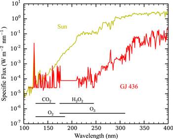
Figure 1. The spectra of the Sun (WMO 1985; yellow) and GJ 436 (France et al. 2013; red) scaled such that the total flux of each is identical to the total flux received by Earth at 1 AU (∼1360 W m−2). The wavelengths at which photolysis of CO2, O2, O3, and H2O2 is most efficient are added for comparison (Tian et al. 2014).
Download figure:
Standard image High-resolution image2.2. Boundary Conditions
The choice of boundary conditions strongly affects the resulting atmospheric composition. The major processes that are typically modeled include hydrogen escape, volcanic outgassing, and surface deposition of oxidants. The rates of these processes, especially the latter two, are highly uncertain. For example, the outgassing flux of water for Earth is 1011–1012 cm−2 s−1 (Fischer 2008), while on Venus it could be as low as 5.5 × 10⁵–107 cm−2 s−1 (Walker et al. 1970; Grinspoon 1993). This is likely due to the hydrodynamic loss of water in Venus's past (Hamano et al. 2013), similar to the conditions experienced by our modeled M dwarf exoplanet. Likewise, the deposition velocity of oxidants, such as O2 and O3, is strongly tied to surface composition and water content. On Earth and Mars, aqueous reactions of molecular oxygen and ozone with ferrous iron, sulfides, and other reducing species act as significant sinks for oxidants, but deposition velocities on Mars could be 10–100 times lower than on Earth due to the reduced surface humidity and differences in surface composition (Zahnle et al. 2008). Therefore, given that our modeled planet could be drier still, and that the crust and upper mantle may already be heavily oxidized, the deposition of oxidants could be severely limited.
If hydrogen escape is in the diffusion-limited regime, then the flux can be expressed as

(Zahnle et al. 2008) where  is the diffusion-limited escape flux, fH is the total mixing ratio of all hydrogen species at the homopause,
  is the binary diffusion coefficient of hydrogen (H or H2) escaping through CO2, and
  is the scale height of species x, where x = H or H2 and CO2. As M dwarfs emit abundant XUV (λ < 121 nm) radiation and highly charged particles that can cause hydrodynamic escape and sputtering, the rate of hydrogen loss could readily reach the diffusion-limited regime (Cohen et al. 2015), though sputtering could be reduced if a strong planetary magnetic field exists (Lammer et al. 2007). On the other hand, the abundance of hydrogen above the homopause is strongly tied to the rate of production from photolysis of water and H2O2, as well as chemistry in the ionosphere (Nair et al. 1994). Thus, in the limit of low atmospheric hydrogen content, the hydrogen escape flux could be much lower than the diffusion-limited flux.
Given the possibility that the outgassing, deposition, and escape fluxes may be low, we will simplify the problem and focus strictly on the effects of high UV flux, low water content, and high CO2-content by assigning zero fluxes to all species for our upper and lower boundary conditions. We make an exception for ions, which have a zero flux upper boundary condition and a fixed concentration of 0 cm−3 at the lower boundary to simulate recombination with electrons at the surface (Nair et al. 1994). This is equivalent to hydrogen escape being balanced by the outgassing of water, with the outgassed oxygen atoms being lost through surface deposition of oxidants. These simplified boundary conditions, which are potentially representative of desiccated terrestrial exoplanets orbiting M dwarfs, will be evaluated in Section 4.1.
2.3. Model Atmosphere
In order to model a CO2-dominated atmosphere we simulate Mars-like atmospheric composition with a surface atmospheric pressure of 1 bar for an Earth-sized planet with Earth's surface gravity. We keep the same (Martian) mixing ratios of atmospheric species as Nair et al. (1994). The pressure P, temperature T, and eddy diffusion coefficient Kzz profiles are shown in Figure 2. The model atmosphere extends from the surface to 100 km altitude with an altitude bin thickness of 1 km. The pressure profile is calculated assuming an ideal gas atmosphere in hydrostatic equilibrium.
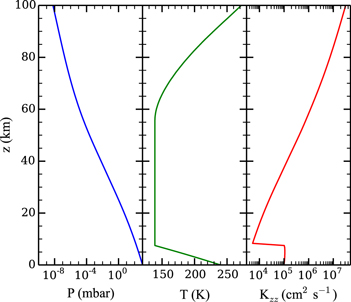
Figure 2. Model atmospheric pressure P (left), temperature T (center), and eddy diffusion coefficient Kzz (right) as functions of altitude z.
Download figure:
Standard image High-resolution imageThe temperature profile is split into the troposphere, the stratosphere/mesosphere, and the thermosphere. The troposphere is assumed to be a dry adiabat with the heat capacity of CO2 as a function of temperature taken from McBride & Gordon (1961) and Woolley (1954). The surface temperature is assumed to be 240 K, accounting for the warming due to 1 bar of CO2 (Kasting 1991). The temperature decreases along the adiabat with increasing altitude until it reaches the planetary skin temperature of 139 K, identical to that of Mars, by assumption (Nair et al. 1994). This places the tropopause of our atmosphere at ∼7.5 km. Above the tropopause the temperature profile is assumed to be isothermal, consistent with previous works (Kasting 1990; Segura et al. 2005, 2007). The temperature increases in the thermosphere above 60 km due to inefficient collisional cooling, and the temperatures are calculated by assuming that the temperature–pressure relationship is identical in the thermospheres of both our model atmosphere and Nair et al. (1994)'s model atmosphere. This assumption is valid given the density (and thus pressure) dependence of collisional cooling (López-Puertas & Taylor 2001). As the pressure profile depends on the temperature profile, we iterate between the two until convergence.
The eddy diffusion coefficient as a function of altitude is calculated assuming free convection (Gierasch & Conrath 1985),

where H is the scale height given by  , R is the universal gas constant, σ is the Stefan–Boltzmann constant, μ is the atmospheric molecular weight, which is assumed to be identical to that of CO2, ρ is the atmospheric mass density, Cp is the atmospheric heat capacity, and L is the mixing length defined with respect to the convective stability of the atmosphere (Ackerman & Marley 2001),

where Γ is the lapse rate and Γa is the adiabatic lapse rate. As with Ackerman & Marley (2001), we set a lower bound for L of 0.1H in the radiative regions of the atmosphere. Using Equations (1) and (2), we find a surface eddy diffusion coefficient value of 3.4 × 107 cm2 s−1, which is more than twice as high as in previous studies where a value of 105 cm2 s−1 is often used (e.g., Nair et al. 1994; Segura et al. 2007). This is likely due to the equations' assumption of free convection breaking down in the presence of a solid surface. Therefore, we scale the entire profile by a constant factor such that the surface value is 105 cm2 s−1.
The temperature, pressure, and eddy diffusion coefficient profiles are held constant with time throughout the simulation, even when the atmospheric composition changes drastically. We will discuss how a self-consistent atmospheric model may impact our results in Section 4.3.
2.4. Atmospheric Hydrogen and Oxygen Content
The hydrodynamic loss of water leads to an atmosphere depleted in hydrogen, which is mostly bound in H2 and H2O in our model. To simulate such depletion we decrease the initial water content of the atmosphere such that it is undersaturated at all altitudes. Using the expression of Lindner (1988) for the temperature-dependent saturation vapor pressure of water we find the minimum value of the saturation water vapor mixing ratio of our model atmosphere to be 1.675 × 10⁻⁵ ppm at the tropopause, where the temperature is 139 K. We then vary the H2 content to investigate the result of different degrees of hydrogen depletion in the atmosphere. We simulate six cases, with total atmospheric H mole fractions  of (1) 26 ppm, (2) 2.6 ppm, (3) 0.27 ppm, (4) 0.032 ppm, (5) 0.0088 ppm, and (6) 0.0065 ppm. f(H)tot is defined as the number of hydrogen atoms in the atmosphere divided by the total number of atoms in the atmosphere. By comparison, the H mole fraction of Venus is 14 ppm (Miller-Ricci et al. 2009).
We assume that the excess oxygen produced from water depletion is taken up by the crust and upper mantle during the Runaway Greenhouse phase, when a magma ocean may have formed on the surface that would have acted as an extremely efficient oxygen sink (Hamano et al. 2013; Luger & Barnes 2015). The resulting atmosphere would then be low in oxygen, while the crust and upper mantle compensate by being oxidized.
3. RESULTS
Despite the low water content of our model atmosphere, >50% of the atmospheric CO2 present at the beginning of our simulations is retained. We find that this results from the actions of CO2-regenerating catalytic cycles that rely on H2O2 and O3 instead of H2O, which arise due to the low M dwarf NUV flux limiting H2O2 and O3 destruction by photolysis. Nonetheless, abiotic O2 and O3 column mixing ratios up to 20% and 1 ppm, respectively, can be produced from CO2 photolysis, giving rise to potential false positives when using O2 or O3 as the signature of biological photosynthesis.
Figure 3 shows the steady state mixing ratios of several species in our model atmosphere as a function of altitude after 10 Gyr of evolution. The long-lived species, such as CO2, CO, O2, H2, H2O, and H2O2, tend to be well mixed below the homopause (∼50 km in our model atmosphere). Above the homopause, (1) CO2 is depleted due to photolysis, which in turn produces an excess of CO and O2, (2) the H2 mixing ratio increases due to molecular diffusion, and (3) H2O and H2O2 are fairly well-mixed, as most of their chemistry takes place at lower altitudes. The short-lived species, as expected, are not well mixed: O3 and HO2 both show clear mixing ratio maxima near the homopause due to their high production rates there, while H and OH are only abundant above the homopause due to their rapid removal below.
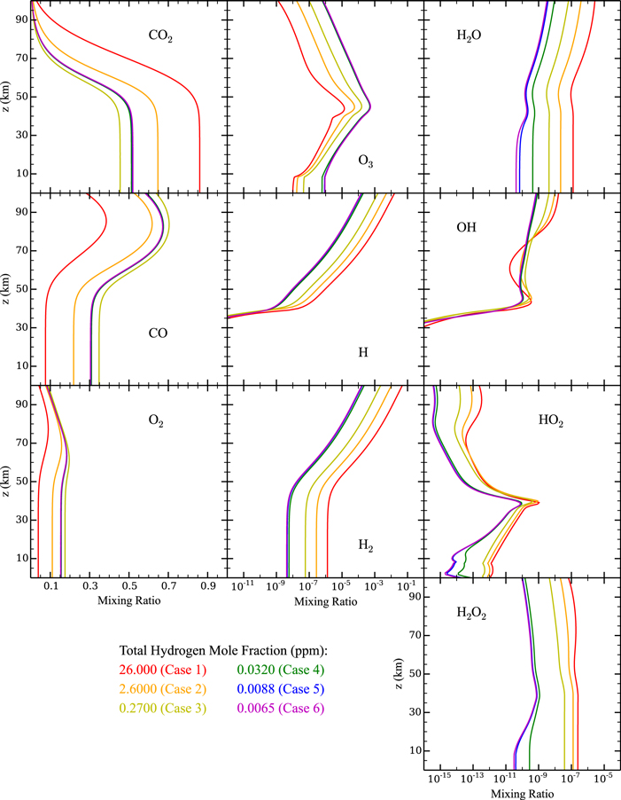
Figure 3. Mixing ratio profiles of CO2, CO, O2, O3, H, H2, H2O, OH, HO2, and H2O2 for Cases 1 (red), 2 (orange), 3 (yellow), 4 (green), 5 (blue), and 6 (magenta). Note the different x-axis values for the three different columns. For many of the species, the curves for cases 4, 5, and 6 overlap each other.
Download figure:
Standard image High-resolution imageFigure 3 also shows a clear trend in the mixing ratios of these species as the atmospheric hydrogen content is varied. For example, as the hydrogen content drops, the hydrogen species' mixing ratios also decrease, while the O3 mixing ratio increases. This trend is better seen in Figure 4, which shows the column-averaged mixing ratios of the same species as in Figure 3, as a function of the atmospheric hydrogen content. There is a clear trend of decreasing CO2 with decreasing atmospheric hydrogen, eventually reaching a lower limit for cases with hydrogen mixing ratio ∼1 ppm. The high abiotic O2 and CO concentrations of our atmospheres (5%–20% and 10%–40%, respectively) are consistent with previous studies showing the propensity for planets with low atmospheric H2O abundance to lose more CO2 to photolysis than planets with high atmospheric H2O abundance (e.g., Segura et al. 2007). However, we do not lose as much CO2 as the results of Zahnle et al. (2008), which showed that an atmosphere as depleted in water as ours (∼0.6 precipitable microns for our "wettest" case) should be unstable to conversion to CO if irradiated by a Sun-like star. This suggests the existence of alternate chemical pathways aside from S1 that are responsible for regenerating CO2 in low H2O, initially CO2-dominated atmospheres of terrestrial planets orbiting M dwarfs. These chemical pathways must be such that (1) CO2 still dominates even when H2O concentrations are low, and (2) CO2 is stopped from complete conversion to CO and O2 even when atmospheric hydrogen is severely depleted.

Figure 4. Column-integrated mixing ratios of (top) CO2 (red), CO (green), O2 (blue), (bottom) O3 (yellow), HO2 (orange), H2O2 (dark blue), and OH (magenta) as functions of the total atmospheric hydrogen mole fraction for Cases 1 through 6. This mole fraction is calculated by dividing the number of hydrogen atoms in the atmosphere by the total number of atoms in the atmosphere. The points indicate the results of the actual cases, which are connected by lines. In the bottom panel we show the range in Earth's O3 mixing ratio  (Yung & DeMore 1999). Note the different y-axis scales of the top and bottom panels.
Download figure:
Standard image High-resolution imageFigure 5 shows the rates of several key reactions near the surface of the planet as the hydrogen content of the atmosphere is reduced from panels 1–6, which correspond to Cases 1–6, respectively, as well as the points on the column-averaged mixing ratio curves of Figure 4. As catalytic cycles require one reaction to feed into another, the reactions that make up the cycle must all have the same effective reaction rate, determined by the rate-limiting step. Thus, for Case 1, R2, R4, R6, and R7 form a catalytic cycle below 20 km:


This cycle depends on relatively high concentrations of H2O2, which replaces water as the major reservoir/source of HOx species. The lower panel of Figure 4 shows that the equilibrium H2O2 mixing ratio for the highest H2 case is ∼0.2 ppm, which is ∼20 times higher than the modeled Martian H2O2 mixing ratio from Nair et al. (1994). This buildup of H2O2 is due to its low photolysis rate around M dwarfs. S2 has been considered as a CO2 regeneration pathway for a wet Mars (Parkinson & Hunten 1972; Yung & DeMore 1999), which relies on high H2O2 abundances arising from high H2O abundances.
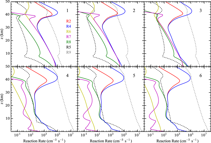
Figure 5. Reaction rates of R2:  (red), R4:
  (blue), R5:
  (black, dotted line), R6:
  (yellow), R7:
  (magenta), R8:
  (green), and R9:
  (gray, dotted line) as functions of altitude in the lower atmosphere for (1) Case 1, f(H)tot ∼ 26 ppm; (2) Case 2, f(H)tot ∼ 2.6 ppm; (3) Case 3, f(H)tot ∼ 0.27 ppm; (4) Case 4, f(H)tot ∼ 0.032 ppm; (5) Case 5, f(H)tot ∼ 0.0088 ppm; and (6) Case 6, f(H)tot ∼ 0.0065 ppm.
Download figure:
Standard image High-resolution imageAs the atmospheric hydrogen content is decreased from Cases 1–3 in Figure 5, the mixing ratios of H2O2 and HO2 decrease (see Figure 4), resulting in a drop in the rates of R6 and R7. Consequently, S2 becomes less efficient at regenerating CO2. This leads to the decrease in CO2 and the increase in CO and O2 shown in Figure 4, which in turn results in the increase in O3. The rise of ozone increases the rate of R8 and its own photolysis reaction R9, which produces an abundance of free oxygen atoms that go into increasing the rate of R5. Eventually, R8 replaces R6 and R7 in S2, forming


which, together with R5, dominates the CO2 regeneration process below 15 km. Case 3 shows the switch from S2 to S3 and R5, where neither process is particularly efficient; this causes the minimum in the CO2 mixing ratio curve in Figure 4. The increase in O3 concentrations goes on to increase the rates of S3 and R5 in Cases 4–6, which in turn explains the upswing in the CO2 mixing ratio seen in Figure 4 for the cases with atmospheric hydrogen content <0.1 ppm. The importance of O3 in S3 and R5 creates a negative feedback, where excess CO2 photolysis produces excess O2 and O3, which then increases the intensity of CO2 regeneration via S3 and R5. This stops further decreases in the CO2 mixing ratio with decreasing atmospheric hydrogen content. S3 has been recognized as a major catalytic cycle for the loss of O3 on M dwarf exoplanets by Grenfell et al. (2013), but they considered an atmosphere similar to that of modern Earth instead of a CO2-dominated atmosphere like that of our model.
Further evidence of the importance of O3 to CO2 regeneration in these low atmospheric hydrogen/water cases is given in Figure 6, which shows molecular fluxes from Case 1 (top) and Case 6 (bottom) near the planet surface for O2, O3, CO, and CO2. The fluxes of Case 1 show a balance between downwelling CO and upwelling CO2, consistent with the conversion from CO to CO2 occurring near the surface by S2. The fluxes of Case 6 are similar, but, in addition, O2 and O3 also have a correspondence, with conversion of O3 to O2 occurring near the surface in keeping with S3.
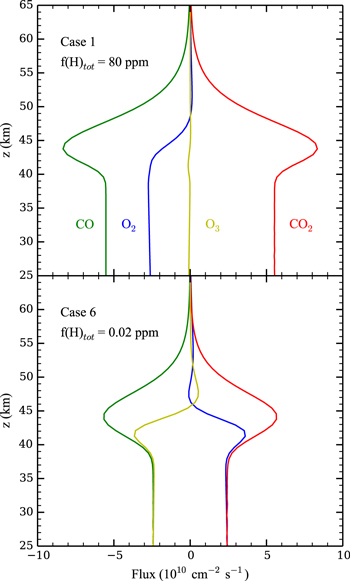
Figure 6. Vertical fluxes of O2 (blue), O3 (yellow), CO2 (red), and CO (green) in the lower atmosphere for Cases 1 (top) and 6 (bottom). Upward fluxes are positive while downward fluxes are negative.
Download figure:
Standard image High-resolution imageFor the cases where the atmospheric hydrogen mixing ratio is <0.05 ppm, as in Cases 5 and 6 of Figure 5, R5 dominates and S3 is reduced, due to low HO2 and OH concentrations. Further decreases in atmospheric hydrogen content are inconsequential since R5 does not depend on any hydrogen species.
The importance of H2O2 and O3 photolysis for S2, S3, and R5 means our results would differ significantly for similar planets around Sun-like stars. Aside from the lack of a prolonged high luminosity pre-main sequence phase, Sun-like stars also emit more strongly in the NUV, resulting in higher rates of H2O2 and O3 photolysis (see Figure 1). Therefore, only a small amount of H2O2 and O3 is necessary to produce the photolysis products needed to regenerate CO2. An alternate simulation of Case 6 that uses a Solar spectrum rather than an M dwarf spectrum yields ∼2% O2 and 4% CO, consistent with the results of previous works that used solar spectra (e.g., Hu et al. 2012). Though these values are lower than our nominal results, they are still ∼100 times higher than that of a non-desiccated planet orbiting a Sun-like star, such as Earth during the Proterozoic eon (Planavsky et al. 2014). This suggests that false positive detections of biosignatures are possible even for desiccated planets around Sun-like stars. These results are also similar to those of Nair et al. (1994) when they only used R5 for CO2 regeneration, though there is more CO2 remaining at equilibrium in our case due to the higher atmospheric density, which increases the rate of R5.
4. DISCUSSION
4.1. Surface Fluxes and Atmospheric Escape
We have assumed zero-flux boundary conditions for all neutral species in our model atmosphere in order to simplify the problem and focus on the effects of high UV flux, low water content, and high CO2-content. This is equivalent to assuming that all fluxes are nonzero, but are in balance with each other. In this section we evaluate this assumption by introducing explicit, balanced fluxes into our model with the goal of determining what surface and escape fluxes are necessary to reproduce our zero-flux results, and thus what planets may possess these atmospheric compositions. The fluxes modeled are the outgassing of H2O, the escape of H and H2 into space, and the surface deposition of O3. O2 deposition is assumed to be zero due to its relatively low reactivity and solubility in water compared to O3 (Sonntag & von Gunten 2012), though its high abundance in the drier cases may increase its significance (see below). Comparisons between the zero-flux and explicit flux models are done using our wettest and driest cases, Cases 1 and 6, respectively. All other run parameters of the models are identical to the corresponding zero-flux cases.
Figure 7 shows the comparison between the mixing ratios derived from the explicit flux model (dashed curves) and that derived from our nominal model (solid curves), for Cases 1 (red) and 6 (blue). There is satisfactory agreement between the two models for almost all of the species, including those vital to the catalytic cycles outlined in Section 3. The major difference between the two models is the reservoir of atmosphere hydrogen. For the zero-flux case, the reservoirs are H2 and H2O2, while in the explicit flux model the hydrogen reservoir is water. This is understandable since water is being actively replenished by outgassing, and the production of H and H2 is dependent on the H2O abundance. This leads to a slight decrease in H and H2 mixing ratios, which further leads to the minor differences in the abundances of the other species.

Figure 7. Mixing ratio profiles of CO2, CO, O2, O3, H, H2, H2O, OH, HO2, and H2O2 for Case 1 of the nominal, zero-flux model (red, solid), Case 1 of the explicit flux model (red, dashed), Case 6 of the nominal model (blue, solid), and Case 6 of the explicit flux model (blue, dashed). Note the different x-axis values for the three different columns.
Download figure:
Standard image High-resolution imageTable 2 shows the escape velocities/fluxes, outgassing fluxes, and surface deposition velocities/fluxes for Cases 1 and 6 of the explicit flux model. The hydrogen escape velocities, which were derived using Case 1 and then applied to Case 6, are consistent with the diffusion-limited escape velocity of hydrogen at Earth's homopause (Hunten 1973). We found that greater escape velocities led to the depletion of hydrogen in the upper atmosphere with respect to the zero-flux results, while lower velocities led to excesses of H and H2 without any changes in the shapes of their profiles. The hydrogen escape flux for Case 1 is consistent with that of Venus (Grinspoon 1993), which is unsurprising given their similar atmospheric hydrogen mole fractions (Miller-Ricci et al. 2009), while Case 6 has much lower escape fluxes, in accordance with its lower atmospheric hydrogen content. The same pattern holds for water outgassing: The flux for Case 1 is similar to that of Venus (5.5 × 10⁵–107 cm−2 s−1), while that of Case 6 is an order of magnitude lower than the given lower limit of the Venus water outgassing flux (Walker et al. 1970). By analogy this could mean that volcanism rates, and thus heat fluxes, are relatively high, but the water content of the lava is much lower. This is consistent with a desiccated upper mantle that lost its hydrogen during the early runaway greenhouse-induced magma ocean phase (Hamano et al. 2013; Luger & Barnes 2015).
Table 2. Boundary Conditions for the Explicit Flux Model that Reproduced the Corresponding Cases for the Zero-flux Model
| Case 1 | Case 6 | |
|---|---|---|
| H escape velocity/flux | 5.5/1.2 × 107 | 5.5/6 × 104 |
| H2 escape velocity/flux | 0.3/2 × 106 | 0.3/3 × 103 |
| H2O outgassing flux | 8 × 10⁶ | 3.3 × 10⁴ |
| O3 deposition velocity/flux | 10−5/2.7 × 106 | 3 × 10⁻¹⁰/1.1 × 104 |
Note. All velocities are given in units of cm s−1 and all fluxes are given in units of cm−2 s−1.
Download table as: ASCIITypeset image
The deposition of oxidants is crucial in determining the oxidative state of the atmosphere. For example, in the work of Zahnle et al. (2008), where H2O2 and O3 are lost to aqueous reactions with ferrous iron and sulfides, the atmosphere tends to be converted entirely to CO. As O3 and H2O2 are crucial to the catalytic cycles we have outlined, it is not surprising that losing them to the surface would result in high CO concentrations, as the efficiency of CO2 regeneration would be vastly decreased. Zahnle et al. (2008) used an O3 deposition velocity of 0.02 cm s−1 for the surface of Mars, which is 3 and 8 orders of magnitude greater than that of our explicit flux results for Cases 1 and 6, respectively. Such low deposition velocities may be consistent with a surface much drier than that of Mars. Zahnle et al. (2008) used a surface relative humidity of water of 17% for their Mars model, which is 320 times higher than the relative humidity for our Case 1 results, and 8.5 × 10⁵ times higher than that of our Case 6 results. Therefore, it is plausible that our deposition velocities are low due to the lack of an aqueous medium within which oxidation can proceed quickly. However, the exact relationship between O3 deposition velocity and relative humidity is unknown, especially for very low water abundances. Alternatively, the planetary surface may be low in ferrous iron and sulfides due to the oxidation resulting from burial of hundreds of bars of oxygen during the aforementioned magma ocean phase.
Similar arguments can be made for O2 deposition. Zahnle et al. (2008) attributed the surface flux of O2 on Mars to UV photostimulated oxidation of magnetite in the presence of trace amounts of water. However, this may be insignificant in our case due to the low UV flux at our model planet's surface, as a result of our thicker atmosphere. Therefore, any O2 flux at the surface is likely due to aqueous reactions with reducing species, as with O3. An alternative simulation of the explicit flux cases using O2 deposition instead of O3 deposition yielded velocities of 3.7 × 10⁻¹² cm s−1 and 3 × 10⁻¹⁵ cm s−1 for Cases 1 and 6, which are 5 and 8 orders of magnitude lower, respectively, than that assumed by Zahnle et al. (2008) for UV photostimulation (4 × 10⁻⁷ cm s−1). Despite the different depositional mechanisms, these differences are similar in magnitude to that of our O3 deposition results. Therefore, as both UV photostimulation and aqueous chemistry require some water, the reduced relative humidity at the surface of our desiccated planet may inhibit O2 deposition by either mechanism just as it does O3 deposition.
These calculations show that terrestrial planets that have experienced severe loss of water and oxidization of the crust and upper mantle, such as planets orbiting in the habitable zones of M dwarfs, can potentially possess an atmosphere similar to our zero-flux results provided that CO2 is abundant in their atmospheres. Consequently, biosignature false positives may be prevalent for planets orbiting in the habitable zone of M dwarfs, and should be taken into consideration in future studies and observation campaigns, as we discuss below.
4.2. Biosignature False Positives
Our results show that O2 mixing ratios of ∼20% and O3 mixing ratios >1 ppm are achievable on H2O-depleted M dwarf terrestrial exoplanets due to photochemistry. These values are similar to that of modern Earth (Yung & DeMore 1999), where the abundant O2 and O3 are produced by biological photosynthesis. In this section we calculate their spectral signatures and consider their impact as potential false positive biosignatures.
Figure 8 shows the thermal emission spectrum of our model atmosphere for Cases 1 (red), 3 (orange), and 6 (green), as generated by the Spectral Mapping Atmospheric Radiative Model (SMART; Meadows & Crisp 1996). We also plot the spectrum of Earth (black) generated by the extensively validated Virtual Planetary Laboratory (VPL) 3D spectral Earth model (Robinson et al. 2010, 2011, 2014), divided by two for comparison. We see immediately that not only are our three cases difficult to separate, but all three cases are very different from Earth's atmosphere as seen in the mid-IR. This is mostly due to the completely different temperature profile assumed and the lack of water vapor, which absorbs at 6.3 and beyond 18 μm, though there is a slight decrease in flux at 6.3 μm for our wettest case (Case 1). Our model atmosphere also lacks methane, which absorbs at 7.7 μm. All spectra feature a deep 15 μm CO2 band, though it is deeper for our model atmosphere due to the cooler stratosphere. Finally, there is weak O3 absorption at 9.7 μm that gets progressively stronger as our model atmosphere becomes drier, but it never approaches the strength of O3 absorption in Earth's atmosphere. The weakness of this absorption is caused by the emission occurring near the surface, such that the brightness temperature of the O3 absorption is similar to the surface temperature, which sets the continuum on either side of the absorption feature. Thus, from the thermal emission there is a clear distinction between actual Earth-like planets and those with abundant atmospheric O2 and O3 caused by low water content and photolysis.
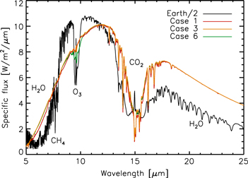
Figure 8. Thermal emission spectra of our model atmosphere for cases 1 (red), 3 (orange), and 6 (green) in the mid-IR compared to that of Earth (black; Robinson et al. 2011), divided by 2 for comparison.
Download figure:
Standard image High-resolution imageFigure 9 shows the normalized reflectance of the same cases as in Figure 8 compared to the reflectance of Earth, again generated by SMART and the VPL Earth model, respectively. A gray surface albedo of 0.15 is assumed for our model planet. We see that the O3 in our model atmosphere can be detected via deep O3 absorption in the NUV similar in strength to O3 absorption in Earth's atmosphere, and our driest case (Case 6) even features a deeper Chappuis band (∼0.6 μm) than Earth. However, whereas all of our cases exhibit a smooth fall-off in reflectance past 0.7 μm, punctuated by CO2 absorption, Earth's reflectance in this region is dominated by water absorption, and thus water again acts as the discriminating species between Earth and our model planet.

Figure 9. Normalized reflectance of our model atmosphere for cases 1 (red), 3 (orange), and 6 (green) from the near-UV to the near-IR compared to that of Earth (black; Robinson et al. 2011). A gray surface albedo of 0.15 is assumed for our model planet.
Download figure:
Standard image High-resolution image
From these comparisons it is clear that the condition necessary to produce abundant O2 and O3 in CO2-dominated atmospheres—low water content—leads to a clear distinction in planetary spectra from those of Earth-like planets via the disappearance of strong water vapor absorption bands. Thus, biologically active, Earth-like planets can be distinguished from the planetary environments presented here using the 0.95 μm water vapor band, the numerous water bands throughout the nearinfrared, or, in the thermal infrared, the 6.3 μm water band, which are all observable by JWST (Beichman et al. 2014). However, caution must be exercised, as high-altitude cloud cover could potentially mask spectral signatures of water vapor.
4.3. Atmospheric Evolution
In our calculations we fix the pressure, temperature, and eddy diffusion coefficient profiles. As we have shown, considerable atmospheric evolution occurs over the 10 Gyr duration of each simulation, including the formation of a significant O3 layer comparable to that of Earth and the conversion of ∼40% of the atmospheric CO2 into CO and O2. Furthermore, the liberation of CO and O from CO2 increases the total number of molecules in the atmosphere, but this should be balanced by the decrease of the molecular weight of the atmosphere from ∼44 to ∼37 g mol−1, thereby increasing the scale height such that local number densities should remain constant. The O3 layer in the stratosphere should raise the temperature such that a temperature inversion results due to heating by photolysis, much like in Earth's stratosphere (Park & London 1974). The decrease in CO2 should result in warming of the stratosphere and mesosphere due to lower rates of radiative cooling (Roble & Dickinson 1989; Brasseur & Solomon 2005), as well as a cooling of the troposphere due to decreased greenhouse effects. Finally, the increase in O2 should result in heating by photolysis in the mesosphere and thermosphere (Park & London 1974). In all, the temperature profile should increase above the tropopause and evolve in shape toward that of Earth, while below the tropopause the temperature will likely decrease.
The reaction rates will change in response to these temperature variations, as most of the reaction rate constants are exponential functions of inverse temperature (Table 1). Of the chemical reactions considered here, R2 (low pressure limit), R3, and R7 have rate constants that are inversely proportional to temperature, while R2 (high pressure limit), R4, R5, and R8 have rate constants that are directly proportional to temperature. Of the photolysis reactions, R1 decreases for decreasing temperatures (Schmidt et al. 2013) and R6 varies negligibly with temperature (Nicovich & Wine 1988). Photolysis of O2 and O3 (R9) decrease slightly with decreasing temperatures (Hudson et al. 1966; Lean & Blake 1981).
The combination of the temperature changes and the response of the reaction rates seem to suggest that (1) CO2 destruction will increase as temperature increases in the stratosphere, (2) CO2 regeneration via S2 and S3 will decrease due to decreasing temperatures in the troposphere, and (3) CO2 regeneration via R5 will also decrease, again due to the cooler troposphere. In other words, the atmosphere may lose much more CO2 if the temperature evolution were taken into account. Quantitatively verifying these hypotheses require running coupled photochemistry and radiative transfer models, which is beyond the scope of this study.
4.4. Condensation
For many of our cases, H2O is supersaturated in the stratosphere/mesosphere by the end of the 10 Gyr model run due to equilibration among the different hydrogen species. The formation of ice clouds would affect the UV radiation environment in the lower atmosphere, but whether the UV is enhanced or attenuated depends on location above or below the clouds, the solar zenith angle, cloud particle properties and distribution, and cloud optical depth. Typical variations in UV intensity on Earth's surface due to clouds are on the order of 25% in either direction while enhancement tends to occur above the clouds (Bais et al. 2006). Given the degree of supersaturation in our wetter runs, however, attenuation is more likely than enhancement below the clouds. This would decrease the H2O2 and O3 photolysis rates and cause an increase in the number densities of these species, which in turn would decrease the efficiency of S2 and R5 while increasing the efficiency of S3. The magnitude to which these pathways change will depend on how much UV is attenuated as a function of wavelength, as well as the variability time scale of the clouds—if this time scale is sufficiently short, it may be irrelevant for the long time scales considered here.
The existence of water ice clouds may also result in heterogeneous chemistry that impacts the stability of CO2 (Atreya & Blamont 1990). For example, observations of high O3 mixing ratios over the northern polar region of Mars during northern spring is likely due to the uptake of HOx radicals by cloud particles (Lefèvre et al. 2008). If similar processes occurred in our model atmosphere, then the decrease in HOx species would reduce the efficiency of S2 and S3, while the buildup in O3 would increase the efficiency of S3 and R5. As S2 is responsible for the highest rate of CO2 regeneration, inclusion of heterogeneous chemistry will likely result in reduced amounts of CO2, even when the atmospheric hydrogen content is relatively high. This is consistent with simulations of the Martian atmosphere that included heterogeneous chemistry (Atreya & Gu 1994; Lefèvre et al. 2008). The magnitude of these effects will depend on the reactive surface area of the cloud particles and the amount of condensable water vapor in the atmosphere.
In drier cases, the lack of significant cloud formation and rainout may produce a substantial silicate dust layer, as in the near-surface atmosphere of Mars (Hamilton et al. 2005). These particles may also participate in heterogeneous chemistry and UV attenuation (Atreya & Gu 1994), though the magnitude of the effect is likely less than that of water ice particles (Nair et al. 1994).
5. SUMMARY AND CONCLUSIONS
We have investigated the stability of H2O—depleted, CO2—dominated atmospheres of terrestrial exoplanets orbiting near the outer edge of the habitable zones of M dwarfs. These atmospheres may be common due to the desiccation and oxidation of the outer layers of these planets during the host stars' pre-main sequence, when it is much more luminous than later in its evolution. We found that these atmospheres are stabilized against photolytic conversion to CO by a series of catalytic cycles and reactions. On Mars, CO2 is maintained through the generation of free hydrogen via water photolysis leading to the oxidation of CO by HOx species. By comparison, for a planet orbiting an M dwarf with severe water depletion, H2O2 photolysis dominates as the main driver of CO2 regeneration due to the lower NUV fluxes of M dwarfs leading to a buildup of H2O2. This cycle is capable of maintaining 80%–90% of the original CO2 content of the atmosphere. However, for atmospheric hydrogen content <1 ppm, H2O2 and HO2 concentrations decrease and the H2O2 cycle (S2) breaks down, resulting in decreasing CO2 and increasing O2 and CO. The rise in O2 leads to higher O3 mixing ratios, which can now participate in the CO2 regeneration process. Due to the low HO2 concentrations, the O3 cycle (S3) can only maintain half of the CO2 in the original atmosphere. If the atmospheric hydrogen content is <0.1 ppm, any reactions involving H-species such as H or HO2 become irrelevant, and the spin-forbidden recombination reaction R5 dominates. This reaction is actually more effective than S3, as O3 (the source of O) increases in abundance as H decreases, and thus only 40% of the atmospheric CO2 is converted to CO and O2. These values may be subject to change given different atmospheric temperatures or surface pressures, but these catalytic cycles and reactions are likely general due to their self-limiting nature, i.e., if one catalytic cycle is inefficient, then another will take over.
Our model produces abundances of abiotic O2 and O3 comparable to that produced by photosynthetic organisms on modern Earth. This is due to our assumption of a low-H2O atmosphere and dry surface, which decreases the CO2 regeneration rate and the surface deposition rate of oxidizing species. These conditions may be applicable to terrestrial exoplanets in the habitable zones of M dwarfs (Luger & Barnes 2015). The high mixing ratios of O2 and O3 can potentially pose as false positives in the search for biosignatures, but a simultaneous search for water vapor could potentially differentiate between an actual Earth-like planet with biologically mediated atmospheric disequilibrium from a water-depleted planet with atmospheric disequilibrium caused by photochemistry. However, cloud cover can dilute this effect by decreasing the strength of water features. Meanwhile, if surface deposition were significant, then the catalytic cycles would break down due to loss of O3 to the surface resulting in low O2 and O3 abundances. This would lead to much greater losses of CO2 and ultimately the formation of a CO atmosphere.
The sensitivity of these results to temperature changes and clouds is highly complex and nonlinear, owing to the unknowns in UV-cloud radiative transfer, heterogeneous chemistry, and the feedback between temperature and reaction rates. A coupled photochemical and radiative transfer model may be necessary to fully elucidate the evolution of these exotic atmospheres.
We thank K. Willacy, M. Allen, and R. L. Shia for assistance with the setting up and running of the KinetgenX code. We thank V. Meadows and R. Barnes for their valuable inputs. This research was supported in part by the Venus Express program via NASA NNX10AP80G grant to the California Institute of Technology, and was performed as part of the NASA Astrobiology Institute's Virtual Planetary Laboratory Lead Team, supported by NASA through the NASA Astrobiology Institute under solicitation NNH12ZDA002C and Cooperative Agreement Number NNA13AA93A. Support for R.H.ʼs work was provided in part by NASA through Hubble Fellowship grant #51332 awarded by the Space Telescope Science Institute, which is operated by the Association of Universities for Research in Astronomy, Inc., for NASA, under contract NAS 5-26555. Part of the research was carried out at the Jet Propulsion Laboratory, California Institute of Technology, under a contract with the National Aeronautics and Space Administration.