


ABSTRACT
Previously we used the Nearby Supernova Factory sample to show that Type Ia supernovae (SNe Ia) having locally star-forming environments are dimmer than SNe Ia having locally passive environments. Here we use the Constitution sample together with host galaxy data from GALEX to independently confirm that result. The effect is seen using both the SALT2 and MLCS2k2 lightcurve fitting and standardization methods, with brightness differences of 0.094 ± 0.037 mag for SALT2 and 0.155 ± 0.041 mag for MLCS2k2 with RV = 2.5. When combined with our previous measurement the effect is 0.094 ± 0.025 mag for SALT2. If the ratio of these local SN Ia environments changes with redshift or sample selection, this can lead to a bias in cosmological measurements. We explore this issue further, using as an example the direct measurement of H0. GALEX observations show that the SNe Ia having standardized absolute magnitudes calibrated via the Cepheid period–luminosity relation using the Hubble Space Telescope
originate in predominately star-forming environments, whereas only ∼50% of the Hubble-flow comparison sample have locally star-forming environments. As a consequence, the H0 measurement using SNe Ia is currently overestimated. Correcting for this bias, we find a value of  70.6 ± 2.6 km s−1 Mpc−1 when using the LMC distance, Milky Way parallaxes, and the NGC 4258 megamaser as the Cepheid zero point, and 68.8 ± 3.3 km s−1 Mpc−1 when only using NGC 4258. Our correction brings the direct measurement of H0 within ∼1 σ of recent indirect measurements based on the cosmic microwave background power spectrum.
Export citation and abstract BibTeX RIS
1. INTRODUCTION
Empirically standardized Type Ia supernovae (SNe Ia) have been developed into powerful distance indicators. Their use in deriving the expansion history of the universe led to the discovery of the acceleration of the cosmological expansion (Perlmutter et al. 1999; Riess et al. 1998). They also have proven to be important in accurately measuring the local Hubble constant, H0. The sample of events in nearby host galaxies within the range of Cepheid and maser calibration is growing, and these can be coupled to other SNe Ia at redshifts where host peculiar motions are negligible in comparison to the current cosmic expansion rate. For instance the SH0ES program (Riess et al. 2011, hereafter SH0ES11) has reached a quoted precision of 3% on the measurement of H0 using SNe Ia, reporting a value of 73.8 ± 2.4 km s−1 Mpc−1. Subsequently, Humphreys et al. (2013) adjusted the distance to the NGC 4258 megamaser, used as one of the Cepheid zero points by SH0ES11, which reduced H0 to 72.7 ± 2.4 km s−1 Mpc−1. More recently, Efstathiou (2014) re-examined the Cepheid analysis of SH0ES11 and made an additional small adjustment, to H0 = 72.5 ± 2.5 km s−1 Mpc−1. Similarly, the HST Key Project and Carnegie Hubble Project (Freedman et al. 2001, 2012) have relied heavily on SNe Ia to obtain their result of 74.3 ± 2.1 km s−1 Mpc−1.
The value of H0 has become the center of attention recently with the Planck collaboration publication of a smaller, indirect, measurement of H0 = 67.3 ± 1.2 km s−1 Mpc−1 (Planck Collaboration et al. 2014) based on modeling the cosmic microwave background (CMB) power spectrum. For a flat ΛCDM cosmology this constitutes a 2.4 σ tension with the original SH0ES11 direct measurement. This tension is reduced to 1.9σ when including the updates by Humphreys et al. (2013) and Efstathiou (2014). (See Bennett et al. 2014 for a discussion of this tension and its consequences for cosmology.)
In this paper, we examine the possibility of as-yet-unaccounted-for environmental dependencies affecting SNe Ia, and the potential for bias in the direct measurement of H0. Concerns of potential environmental biases in standardized SN Ia distances arise from both theoretical and empirical studies. A wide range of progenitor configurations and explosion scenarios remain in contention. But in all progenitor models, variation is allowed due to differences in mass, composition, geometrical configuration, and evolutionary stage. Statistically, the incidence of these factors is modulated by the parent stellar population, i.e., the progenitor environment. The theoretical predictions remain far too uncertain to be applied directly for precision cosmological analyses, motivating empirical studies of the association between SN properties and environment.
Empirical studies using global or nuclear host-galaxy properties have been fruitful in revealing environmental dependencies that remain even after SNe Ia are standardized using their lightcurve widths and colors (e.g., Kelly et al. 2010; Sullivan et al. 2010; Lampeitl et al. 2010; Gupta et al. 2011; D'Andrea et al. 2011). The clearest relation found in these studies is a "step" in the mean Hubble residual between SNe Ia in hosts above and below a total stellar mass of 1010.2 ± 0.5 M☉ (Childress et al. 2013a). While there is a predicted trend of SN Ia luminosity with metallicity via the effects of neutronization (Höflich et al. 1998; Timmes et al. 2003; Kasen et al. 2009), this observed change as a function of host mass via the mass–metallicity relation is simply too fast. However, there is a strong transition between predominately passive to predominately star-forming (SF) galaxies around this stellar mass, and a very general star-formation-driven model fits the mass step well (Childress et al. 2013a).
While such studies based on global host properties have been productive, they leave unanswered the deeper connection to the progenitor. Global measurements of environmental properties are light-weighted quantities, and thus will be skewed toward the environmental properties of galaxy cores. Slit or fiber spectroscopy is even more biased in this regard as the outer regions of the galaxy, in which an SN progenitor may have formed, are either geometrically deweighted (when integrating along a slit) or excluded altogether (when using a fiber). Of course the degree of this bias depends on the—generally unknown—projected radial gradients of age and metallicity in the SN hosts. This can be ameliorated in part by measuring host properties in annuli at the same galactocentric radius as the SN (Raskin et al. 2009).
In Rigault et al. (2013, hereafter R13) we went a step further and focused on the immediate environment surrounding each SN. A key insight that motivated the R13 study was the realization that the small velocity dispersion of young stars (∼3 km s−1; de Zeeuw et al. 1999; Portegies Zwart et al. 2010; Röser et al. 2010) means that the youngest SN Ia progenitors would not have had time to migrate from the neighborhood where they were formed. Thus, if SNe Ia do indeed have a rapidly falling—1/t—delay time distribution (see, e.g., Maoz et al. 2012), then only a minority of SNe Ia would be superimposed on a geometrical region of their host that is unrelated to their birth environment. Even for such cases, the global environment would need to be dramatically different than the progenitor formation environment to produce an incorrect characterization of environment properties.
Galaxy simulations show only limited radial and azimuthal mixing in disk galaxies over 1 Gyr timescales, and the coherence over 10 Gyr is still surprisingly good for a large fraction of stars (see, e.g., Roskar et al. 2008a, 2008b, 2012; Brunetti et al. 2011; Bird et al. 2012; Di Matteo et al. 2013). For this reason, a local measurement was almost certain to be superior to a global measurement in terms of isolating environmental variables influencing progenitor properties.
Using Nearby Supernova Factory observations (SNfactory; Aldering et al. 2002), R13 showed that SN Ia standardized magnitudes depend on the star formation activity of the SN environment within a projected radius of 1 kpc, as traced by Hα surface brightness. After standardization using SALT2 (Guy et al. 2007), SNe Ia in locally passive environments (designated as Ia ) are on average brighter than SNe in locally SF regions (designated as Iaα) by
  0.094 ± 0.031 mag.16 Since the underlying connection is with star formation rather than the Hα emission itself, we refer to this effect as the local star-formation bias, or LSF bias for short.
R13 connected the LSF bias to the host-mass step by noting that few of the Ia in the SNfactory sample occur in low-mass hosts, leading to a shift in mean brightness with host mass that is driven by the changing fraction of star formation. However, this also implies that simply correcting for the host-mass step will not necessarily correct the local star-formation bias (see Appendix A of R13 for details). As discussed there, since the fraction of SNe Ia from passive regions is expected to decrease with lookback time, such a magnitude difference can introduce a redshift-dependent bias in distance measurements based on SNe Ia. More subtle perhaps is the fact that even variations in the ratio of passive to SF hosts within nearby SNe Ia samples may also induce a bias. This may introduce systematic errors into peculiar velocity measurements via the star formation–density relation, and could bias the direct measurement of H0 when the SN distance ladder relies on distance indicators tied to specific stellar populations.
Given this, confirmation of the local star-formation bias and its impact on the cosmological parameters—notably w and H0—are of paramount importance. The bias on w was examined R13; potential bias on H0 is a subject of this paper. We split our investigation into two parts. The first part of the paper, Section 2, presents our main analysis confirming the LSF bias in the independent Constitution SN Ia data set compiled in Hicken et al. (2009b, hereafter H09). In the second part of the paper, Section 3, we investigate how the LSF bias affects the measurement of H0 using SNe Ia. We conclude in Section 4.
2. CONFIRMATION OF A LOCAL STAR-FORMATION BIAS
In this part of the paper, we describe the data set, measurements and results of our investigation of the LSF bias using an SN Ia data set largely independent of that used in R13. Section 2.1 describes the sample selection, including sources of attrition. Section 2.2 discusses the measurements, including correction for dust extinction and the choice of local metric aperture size. Sections 2.3 and 2.4 present our main results regarding confirmation of the LSF bias and the robustness of the results. In Section 2.5 we discuss the structure of the Hubble residuals relative to the bimodal model of R13. Some finer technical aspects of these measurements are given in Appendices A–D for the benefit of interested readers.
2.1. The Comparison Sample
In order to confirm the LSF bias previously detected in the SNfactory sample we need an independent nearby Hubble-flow sample for which it is possible to compare SALT2-standardized magnitudes between SNe Ia from locally SF and passive environments. The compilation of H09 has been used previously for a number of cosmological analyses (e.g., H09; Kessler et al. 2009; Rest et al. 2014; Riess et al. 2009, 2011) and only six of the SNe Ia have been studied in R13 already. For the nearby Hubble flow range of 0.023 < z < 0.1 (as used, e.g., by SH0ES11), we find that the H09 compilation contains 110 such Hubble-flow SNe Ia. Because the H09 sample was constructed for cosmological applications, peculiar SNe Ia or those with large extinction or poor lightcurve fits have already been removed. Thus, the H09 compilation appears to be quite suitable for an independent measurement of the LSF bias, provided a suitable set of local star-formation measurements can be obtained. A 0.14 ± 0.07 mag offset between E/S0 and Sc/Sd/Irr morphological types in this sample was identified by H09, thus a first comparison between bias revealed by morphological versus local star-formation indicators will be possible.
In the case of R13, it was possible to obtain sensitive measurements of the local Hα surface brightness as a direct by-product of the SuperNova Integral Field Spectrograph (SNIFS) observations conducted by the SNfactory. Conventional slit spectroscopy or imaging photometry, as employed for the SN Ia follow-up programs compiled in H09, does not afford any robust parallel quantitative measurement of local star formation. Furthermore, archival Hα imaging is quite limited for the galaxies in the H09 compilation. Thus, suitable Hα data for measuring the LSF bias in the H09 sample are not currently available.
The far-ultraviolet (FUV) luminosity is another well-established SF indicator. Previously, we used this along with optical data to characterize the global star formation activity of SNfactory SNe Ia host galaxies (Childress et al. 2013a, 2013b), while Neill et al. (2009) did the same for many host galaxies in the H09 sample.
This led us to investigate the availability of sufficiently deep GALEX FUV imaging for the H09 host galaxies. We found that 92 out of the 110 H09 Hubble-flow SN Ia host galaxies have UV coverage from the GALEX GR6/7 data release in the MAST archive,17 and that these data have sensitivity sufficient to classify SN Ia environments following the scheme of R13 for most hosts. (Observations from the CAUSE phase of the GALEX mission were not considered due to their inhomogeneous nature.) We also investigated the available coverage from SWIFT. There the overlap with the H09 Hubble-flow subsample was too small to be useful and all but two cases had GALEX coverage already, and thus we decided not to use the SWIFT data at this time. We therefore proceed to examine the LSF bias using a combination of the nearby Hubble-flow SN Ia subset from H09 and UV data from GALEX.
As a start, we examine any biases that may arise from excluding the subset of SNe Ia lacking GALEX coverage. GALEX was ostensibly an all-sky imaging survey (AIS) reaching a 5 σ point source depth of mFUV = 19.9 AB mag (Morrissey et al. 2007). However, partway through the mission the FUV detector failed to function, leading to incomplete FUV coverage. In addition, bright stars were avoided in order to prevent damage to the GALEX detectors, leaving coverage gaps concentrated toward the Galactic plane region, which SN surveys avoid anyway. GALEX also conducted deeper surveys—the Medium Imaging Survey (MIS) covering 1000 deg2 to mFUV = 23.5 AB mag and the Deep Imaging Survey (DIS) covering 80 deg2 to mFUV = 25.0 AB mag—in fields coincident with other extragalactic surveys. These solid angles are much smaller than the sky coverage typical of nearby SN surveys, and thus constitute a fairly random sampling. Since these variations in GALEX coverage with respect to sky location or proximity to bright stars are completely decoupled from characteristics of nearby SN searches, there is no a priori expectation for a bias between SNe Ia in hosts with and without GALEX coverage. Indeed, application of Kolmogorov–Smirnov tests indicates that lightcurve stretch, color and standardized Hubble residual distributions of the 18 SNe Ia without GALEX observations are completely compatible with those having GALEX coverage, giving similarity probabilities greater than 16% for all comparisons.
Next we apply the selection criteria used in R13, which we follow in order to provide the best possible comparison to that study. In R13 we eliminated SNe Ia spectroscopically classified as 91T-like according to Scalzo et al. (2012) due to the possibility that they may be so-called super-Chandrasekhar SNe Ia and therefore not representative of SN cosmology samples. In Appendix B.1 we provide details of this selection process, which resulted in the elimination of three 91T-like SNe Ia, one of which lacked GALEX FUV coverage anyway. R13 also removed highly inclined hosts; as discussed in more detail in Appendix B.2, for FUV observations this helps avoid both potential false-positive and false-negative environmental associations. We identified seven SN host galaxies with i > 80°; SN 1992ag, SN 1995ac, SN 1997dg, SN 1998eg, SN 2006ak, SN 2006cc and SN 2006gj, and removed them from our baseline analysis.
As a result of these sample selection procedures, which are summarized in Table 1, our baseline analysis will utilize 77 hosts when using Hubble residuals based on SALT2 and 83 hosts when using MLCS2k2 (Jha et al. 2007) Hubble residuals. This sample size compares favorably with the sample of 82 hosts used in R13 to discover the LSF bias.
Table 1. Composition of the Comparison Sample
| Number of SNe Ia | ||||
|---|---|---|---|---|
| SALT2 | MLCS2k2 | |||
| RV = 1.7 | RV = 2.5 | RV = 3.1 | ||
| H09 sample within 0.023 < z < 0.1 | 104 | 110 | 105 | 109 |
| − No GALEX data | 18 | 18 | 15 | 16 |
| − 91T-like | 3 | 2 | 2 | 3 |
| − Highly inclined host | 7 | 7 | 7 | 7 |
| Main analysis comparison sample | 77 | 83 | 81 | 84 |
Notes. Our MLCS2k2 RV = 2.5 subsample is constructed from the intersection of the H09 RV = 1.7 and RV = 3.1 samples. The 91T-like SN1999gp has no GALEX data, and no MLCS2k2 RV = 1.7 measurement in H09.
Download table as: ASCIITypeset image
2.2. Measurement of Local Star Formation
2.2.1. FUV and Hα as Star-formation Indicators
Massive short-lived O and early B type stars with ≳ 17 M☉ are responsible for the ionizing radiation that generates Hα emission, while FUV emission is produced by O- through late-B stars with ≳ 3 M☉. Detection of UV light is therefore an indication of star formation within the preceding 100 Myr (see Calzetti 2013 for a detailed review) and FUV and Hα emission are strongly coupled. This makes them consistent and commonly used star formation indicators (see, e.g., Sullivan et al. 2000; Bell & Kennicutt 2001; Salim et al. 2007 and generally Lee et al. 2009, 2011 and references therein).
Like Hα, the FUV flux drops dramatically with the age of the stellar population. In simple stellar-population instantaneous-burst models that account for the late-time contribution of hot subdwarfs, the FUV flux drops by ∼1.4 dex between 10 Myr and 100 Myr, and then another ∼3 dex from 100 Myr to 1 Gyr (Han et al. 2007; Leitherer et al. 1999). While this is an exceptionally strong signal, it is complicated by dust extinction that is stronger in the FUV than for Hα. This not only weakens the ability to detect star formation, but adds non-negligible uncertainty arising from the extinction correction.
There is also a diffuse FUV component, analogous to the diffuse Hα commonly observed in nearby spiral galaxies. In Appendix D we provide further details concerning this diffuse emission source, along with our examination of its potential impact. For the equivalent star-formation threshold set in R13 (see below), we find that this component should only marginally affect our classification of SN Ia environments.
After correcting for Galactic and interstellar dust extinction, details of which are discussed in Section 2.2.2, both Hα and FUV indicators can be converted to a star formation rate (SFR) surface density, ΣSFR (in M☉ yr−1 kpc−2):
In this equation,  is the dust-corrected FUV luminosity (in erg s−1 Hz−1) summed over an aperture centered at the SN location having area
  . ΣHα is the local Hα surface brightness (in erg s−1 kpc−2). The redshifts considered here are small (z ∼ 0.03), so the FUV and NUV K-corrections are negligible—typically smaller than the measurement errors (Chilingarian & Zolotukhin 2012). Here we use the usual conversion factors κ1 = 1.08 × 10⁻²⁸ and κ2 = 5.5 × 10−42, as in, e.g., Salim et al. (2007); Kennicutt et al. (2009); Calzetti (2013). Modifications to the initial mass function, metallicity, etc., can alter these conversion factors by ±0.2 dex; see Table 2 of Hao et al. (2011) for examples. As in R13, we do not attempt to perform corrections to face-on quantities due to uncertainty concerning the three-dimensional distribution of star formation in local regions. Even for the extreme case of SNe in the planes of pure disks viewed at random inclinations below our limit of
  , only ∼0.2 dex of additional scatter is introduced.
In R13 we used an Hα surface density threshold of log (ΣHα) = 38.35 dex, corresponding to log (ΣSFR) = −2.9 dex, to split the SNfactory sample into two equal-sized groups. Below this threshold SNe Ia were classified as having a locally passive environment, Ia, and above this threshold they were classified as having a locally SF environment, Iaα. The R13 threshold also happened to be that ensuring a minimum 2σ detection over the SNfactory redshift range, and it was also high enough to limit the impact of miscategorization caused by diffuse Hα emission.
We retain this threshold for the current analysis for consistency with R13. For FUV measurements this threshold is also sufficient to minimize miscategorization due to the aforementioned diffuse FUV light; Boquien et al. (2011) found that for log (ΣSFR) > −2.75 dex interarm regions in M33 are largely suppressed and our threshold is only slightly below this. The mildly non-linear relation observed between Hα and FUV (Lee et al. 2009; Verley et al. 2010) does not affect the placement of this threshold by more than ∼0.1 dex.
To account for measurement errors, rather than simply dividing the SNe Ia into two groups as in R13, we will estimate a probability for each SN,  , giving the chance that its local environment is locally passive. To do so we use the Poisson errors on the measurements of FUV flux and extinction, AFUV (see Section 2.2.2), and calculate the fraction of the resulting log (ΣSFR) distribution that has
  . We have confirmed the appropriateness of using Poisson uncertainties by measuring aperture fluxes for 104 blank sky regions and checking that the results were Poisson-distributed.
2.2.2. Local Dust Correction
Dust is associated with star formation (e.g., Charlot & Fall 2000; Simones et al. 2014; Verley et al. 2010) and so can have a strong impact on the observed UV light around the SN location. The amount of dust depends on many factors such as the geometry, the quantity of metals available to form dust, and dust production and destruction mechanisms and timescales. Nevertheless, for SF galaxies there is a good correlation between FUV−NUV color and the amount of FUV dust-absorption, AFUV. Here we use the relation given in Equation (5) of Salim et al. (2007) to estimate AFUV. (See Conroy et al. 2010 for examples of several alternative extinction relations.) Since this correction is only appropriate for SF environments, we face the need to assess whether an environment is SF before knowing whether to correct for extinction.
We start by examining the global SF properties of the SN host galaxies. The association of dust with star-formation suggests that locally passive environments should not require extinction correction, and in R13 we found that globally passive host galaxies are also locally passive. Thus, in most cases it would be inappropriate to apply extinction corrections to the local environments for SNe in globally passive galaxies. One very useful quantitative measure of star-formation activity is the global specific star-formation rate (sSFR). sSFR measurements are available for ∼60% of the host galaxies in our sample. These are based primarily on UV and optical colors (Neill et al. 2009), plus NIR for some (Childress et al. 2013b). Using sSFR, we categorize host galaxies with conclusively low sSFR as globally passive and those with conclusively high sSFR as globally SF. Specifically, to be considered conclusively low or high, we require that the measured sSFR be, respectively, one standard deviation below or above a boundary set at sSFR = −10.5 dex. In Table 2, we designate these as having host types of Pa and SF, respectively. Cases where the sSFR is within one standard deviation of the threshold are designated as ∼Pa and ∼SF, depending on whether their sSFR is, respectively, below or above −10.5 dex.
Table 2. FUV Measurements of the Hubble-flow SN Ia Sample
| Name |  (mag) (mag) |
z | GALEX data | Local | Global | Local | log (ΣSFR) |  |
Cuts | ||||
|---|---|---|---|---|---|---|---|---|---|---|---|---|---|
| SALT | MLCS2k2 | Exp. | FUV | NUV | AFUV | Host | Dust | ||||||
| RV = 1.7 | RV = 2.5 | (s) | (mag) | (mag) | (mag) | Class | Corr. | (M☉ kpc−2 yr−1) | (%) | Applied | |||
| 1990O | −0.14 ± 0.19 | −0.02 ± 0.16 | −0.02 ± 0.16 | 0.031 | 145 | 22.77 ± 0.64 | 24.73 ± 1.68 | 1.9 ± 0.6 | SF | Y |  |
22 | |
| 1990af | −0.13 ± 0.18 | −0.28 ± 0.19 | −0.25 ± 0.20 | 0.050 | 489 | 27.35 ± 10.11 | >21.8 | 2.0 ± 0.6 | Pa | N |  |
100 | |
| 1991U | −0.35 ± 0.20 | ⋅⋅⋅ | ⋅⋅⋅ | 0.033 | 219 | 21.43 ± 0.36 | 20.63 ± 0.10 | 2.2 ± 0.6 | ∼SF | Y |  |
6 | |
| 1992J | −0.27 ± 0.19 | ⋅⋅⋅ | ⋅⋅⋅ | 0.046 | 218 | 26.61 ± 7.93 | 24.22 ± 0.80 | 2.0 ± 0.6 | Pa | N |  |
100 | |
| 1992P | +0.10 ± 0.20 | +0.11 ± 0.17 | +0.14 ± 0.18 | 0.026 | ⋅⋅⋅ | no image | no image | ⋅⋅⋅ | ∼SF | ⋅⋅⋅ | ⋅⋅⋅ | ⋅⋅⋅ | UV |
| 1992ae | −0.08 ± 0.18 | −0.08 ± 0.19 | −0.08 ± 0.20 | 0.075 | 558 | 24.00 ± 0.83 | 23.47 ± 0.24 | 2.0 ± 0.6 | Pa | N |  |
61 | |
| 1992ag | −0.30 ± 0.20 | −0.21 ± 0.18 | −0.23 ± 0.19 | 0.026 | 184 | 19.38 ± 0.11 | 19.20 ± 0.05 | 1.3 ± 0.3 | ∼SF | Y |  |
0 | Incl. |
| 1992bg | ⋅⋅⋅ | −0.01 ± 0.17 | +0.00 ± 0.17 | 0.036 | 199 | 22.23 ± 0.45 | 22.78 ± 0.38 | 1.7 ± 0.5 | SF | Y |  |
10 | |
| 1992bh | +0.12 ± 0.18 | +0.26 ± 0.16 | +0.24 ± 0.17 | 0.045 | 175 | 22.78 ± 0.54 | 22.51 ± 0.28 | 1.9 ± 0.6 | SF | Y |  |
11 | |
| 1992bk | +0.15 ± 0.28 | −0.05 ± 0.23 | −0.03 ± 0.22 | 0.058 | 1021 | 26.28 ± 1.64 | 25.40 ± 0.62 | 2.0 ± 0.6 | Pa | N |  |
100 | |
| 1992bl | −0.05 ± 0.20 | −0.08 ± 0.18 | −0.04 ± 0.17 | 0.043 | 109 | 23.79 ± 1.08 | 27.78 ± 15.79 | 2.0 ± 0.6 | ∼Pa | N |  |
96 | |
| 1992bp | −0.27 ± 0.17 | −0.16 ± 0.15 | −0.13 ± 0.14 | 0.079 | 106 | >20.6 | 27.41 ± 9.45 | 2.0 ± 0.6 | Pa | N | < − 3.0 | 66 | |
| 1992br | +0.11 ± 0.21 | −0.63 ± 0.22 | −0.51 ± 0.24 | 0.088 | ⋅⋅⋅ | no image | no image | ⋅⋅⋅ | Pa | ⋅⋅⋅ | ⋅⋅⋅ | ⋅⋅⋅ | UV |
| 1992bs | +0.20 ± 0.17 | +0.23 ± 0.18 | +0.23 ± 0.19 | 0.063 | 216 | 22.45 ± 0.40 | 23.13 ± 0.32 | 1.6 ± 0.5 | SF | Y |  |
5 | |
| 1993B | −0.11 ± 0.17 | +0.07 ± 0.17 | +0.10 ± 0.17 | 0.071 | 192 | 23.14 ± 0.61 | 22.14 ± 0.21 | 2.1 ± 0.6 | SF | Y |  |
11 | |
| 1993H | ⋅⋅⋅ | −0.25 ± 0.17 | −0.22 ± 0.17 | 0.025 | 137 | 23.05 ± 0.88 | 22.34 ± 0.35 | 2.0 ± 0.6 | SF | Y |  |
39 | |
| 1993O | +0.02 ± 0.17 | +0.11 ± 0.14 | +0.16 ± 0.14 | 0.052 | 215 | >21.1 | 25.08 ± 1.34 | 2.0 ± 0.6 | Pa | N | < − 3.8 | 99 | |
| 1993ac | +0.05 ± 0.19 | +0.06 ± 0.19 | +0.05 ± 0.21 | 0.049 | 224 | 26.19 ± 6.78 | 24.36 ± 0.78 | 2.0 ± 0.6 | Pa | N |  |
98 | |
| 1993ag | −0.05 ± 0.18 | +0.23 ± 0.16 | +0.22 ± 0.16 | 0.050 | ⋅⋅⋅ | no image | no image | ⋅⋅⋅ | Pa | ⋅⋅⋅ | ⋅⋅⋅ | ⋅⋅⋅ | UV |
| 1994M | +0.03 ± 0.20 | −0.01 ± 0.18 | −0.02 ± 0.18 | 0.024 | 109 | >22.5 | 24.97 ± 2.68 | 2.0 ± 0.6 | ∼Pa | N | < − 4.3 | 100 | |
| 1994T | −0.02 ± 0.19 | −0.28 ± 0.16 | −0.20 ± 0.16 | 0.036 | 136 | >21.8 | 25.05 ± 1.93 | 2.0 ± 0.6 | Pa | N | < − 4.3 | 100 | |
| 1995ac | −0.32 ± 0.17 | −0.23 ± 0.13 | −0.27 ± 0.14 | 0.049 | 211 | 23.99 ± 0.91 | 22.83 ± 0.30 | 2.1 ± 0.6 | SF | Y |  |
26 | Incl. |
| 1996C | +0.20 ± 0.20 | +0.32 ± 0.16 | +0.34 ± 0.17 | 0.028 | ⋅⋅⋅ | no image | no image | ⋅⋅⋅ | SF | ⋅⋅⋅ | ⋅⋅⋅ | ⋅⋅⋅ | UV |
| 1996bl | −0.12 ± 0.18 | −0.00 ± 0.15 | −0.01 ± 0.16 | 0.035 | 221 | 22.15 ± 0.35 | 22.18 ± 0.21 | 1.7 ± 0.5 | SF | Y |  |
7 | |
| 1997dg | +0.41 ± 0.19 | +0.38 ± 0.16 | +0.38 ± 0.16 | 0.030 | 488 | 21.63 ± 0.22 | 21.96 ± 0.13 | 1.2 ± 0.4 | ∼SF | Y |  |
5 | Incl. |
| 1998ab | −0.31 ± 0.19 | −0.32 ± 0.16 | −0.37 ± 0.16 | 0.028 | 316 | 20.52 ± 0.23 | 20.36 ± 0.07 | 1.6 ± 0.4 | SF | Y |  |
2 | 91T |
| 1998dx | −0.10 ± 0.18 | −0.15 ± 0.14 | −0.16 ± 0.14 | 0.054 | 153 | >21.3 | 26.29 ± 3.72 | 2.0 ± 0.6 | ∼Pa | N | < − 3.7 | 97 | |
| 1998eg | +0.07 ± 0.21 | +0.09 ± 0.18 | +0.08 ± 0.18 | 0.024 | 166 | 22.87 ± 0.69 | 23.88 ± 0.96 | 1.9 ± 0.6 | ∼Pa | N |  |
100 | Incl. |
| 1999awb | +0.07 ± 0.18 | ⋅⋅⋅ | ⋅⋅⋅ | 0.039 | 322 | 27.66 ± 19.96 | >22.4 | 2.0 ± 0.6 | SF | Y | < − 3.5 | 75 | |
| 1999cc | −0.03 ± 0.18 | −0.05 ± 0.15 | −0.06 ± 0.15 | 0.032 | 137 | 21.93 ± 0.40 | 20.92 ± 0.14 | 2.2 ± 0.6 | SF | Y |  |
9 | |
| 1999ef | +0.24 ± 0.19 | +0.33 ± 0.16 | +0.37 ± 0.16 | 0.038 | 112 | 23.98 ± 1.31 | 23.14 ± 0.52 | 2.0 ± 0.6 | SF | Y |  |
40 | |
| 1999gp | +0.01 ± 0.19 | ⋅⋅⋅ | ⋅⋅⋅ | 0.026 | ⋅⋅⋅ | no image | no image | ⋅⋅⋅ | SF | ⋅⋅⋅ | ⋅⋅⋅ | ⋅⋅⋅ | 91T UV |
| 2000bh | −0.12 ± 0.21 | +0.00 ± 0.20 | +0.02 ± 0.20 | 0.024 | ⋅⋅⋅ | no image | no image | ⋅⋅⋅ | SF | ⋅⋅⋅ | ⋅⋅⋅ | ⋅⋅⋅ | UV |
| 2000ca | −0.16 ± 0.20 | −0.15 ± 0.16 | −0.11 ± 0.16 | 0.025 | 3362 | 20.93 ± 0.07 | 20.21 ± 0.02 | 2.6 ± 0.2 | SF | Y |  |
0 | |
| 2000cf | +0.18 ± 0.18 | +0.17 ± 0.14 | +0.18 ± 0.15 | 0.036 | 204 | 21.76 ± 0.46 | 21.22 ± 0.13 | 2.0 ± 0.6 | SF | Y |  |
8 | |
| 2001ah | −0.10 ± 0.18 | −0.03 ± 0.17 | +0.02 ± 0.16 | 0.058 | ⋅⋅⋅ | no image | no image | ⋅⋅⋅ | SF | ⋅⋅⋅ | ⋅⋅⋅ | ⋅⋅⋅ | UV |
| 2001az | +0.05 ± 0.18 | −0.04 ± 0.15 | +0.00 ± 0.15 | 0.041 | ⋅⋅⋅ | no image | 22.62 ± 0.28 | ⋅⋅⋅ | SF | ⋅⋅⋅ | ⋅⋅⋅ | ⋅⋅⋅ | UV |
| 2001ba | +0.10 ± 0.19 | +0.08 ± 0.15 | +0.13 ± 0.14 | 0.030 | 107 | 22.38 ± 0.63 | 22.53 ± 0.42 | 1.9 ± 0.6 | SF | Y |  |
16 | |
| 2001eh | −0.05 ± 0.18 | +0.12 ± 0.13 | +0.14 ± 0.13 | 0.036 | ⋅⋅⋅ | no image | no image | ⋅⋅⋅ | SF | ⋅⋅⋅ | ⋅⋅⋅ | ⋅⋅⋅ | UV |
| 2001gb | ⋅⋅⋅ | +0.04 ± 0.23 | ⋅⋅⋅ | 0.027 | ⋅⋅⋅ | no image | no image | ⋅⋅⋅ | SF | ⋅⋅⋅ | ⋅⋅⋅ | ⋅⋅⋅ | UV |
| 2001ic | ⋅⋅⋅ | −0.10 ± 0.21 | ⋅⋅⋅ | 0.043 | 208 | >21.8 | 23.89 ± 0.66 | 2.0 ± 0.6 | Pa | N | < − 5.8 | 100 | |
| 2001ie | −0.02 ± 0.20 | −0.03 ± 0.18 | −0.04 ± 0.20 | 0.031 | 103 | >22.0 | 25.22 ± 2.40 | 2.0 ± 0.6 | Pa | N | < − 3.9 | 100 | |
| 2002G | +0.04 ± 0.24 | −0.40 ± 0.35 | −0.41 ± 0.38 | 0.035 | 173 | 23.36 ± 0.72 | 22.07 ± 0.22 | 2.1 ± 0.6 | SF | Y |  |
24 | |
| 2002bf | −0.20 ± 0.21 | +0.13 ± 0.18 | +0.11 ± 0.19 | 0.025 | 112 | 22.04 ± 0.47 | 20.40 ± 0.12 | 2.5 ± 0.6 | ∼SF | Y |  |
12 | |
| 2002bz | +0.11 ± 0.24 | −0.01 ± 0.18 | ⋅⋅⋅ | 0.038 | ⋅⋅⋅ | no image | no image | ⋅⋅⋅ | SF | ⋅⋅⋅ | ⋅⋅⋅ | ⋅⋅⋅ | UV |
| 2002ck | +0.02 ± 0.19 | +0.02 ± 0.17 | +0.03 ± 0.17 | 0.030 | ⋅⋅⋅ | no image | no image | ⋅⋅⋅ | ∼SF | ⋅⋅⋅ | ⋅⋅⋅ | ⋅⋅⋅ | UV |
| 2002de | +0.06 ± 0.20 | +0.12 ± 0.16 | +0.08 ± 0.18 | 0.028 | 110 | 20.51 ± 0.23 | 19.80 ± 0.09 | 2.2 ± 0.5 | SF | Y |  |
3 | |
| 2002hd | −0.31 ± 0.19 | −0.34 ± 0.17 | −0.33 ± 0.18 | 0.036 | 112 | 23.10 ± 0.80 | 21.59 ± 0.22 | 2.1 ± 0.6 | Pa | N |  |
94 | |
| 2002he | +0.08 ± 0.21 | −0.08 ± 0.19 | −0.06 ± 0.19 | 0.025 | 110 | 25.01 ± 3.10 | 23.28 ± 0.68 | 2.0 ± 0.6 | ∼SF | N |  |
100 | |
| 2002hu | −0.11 ± 0.18 | −0.03 ± 0.13 | +0.00 ± 0.13 | 0.038 | 128 | 25.03 ± 2.68 | 22.90 ± 0.44 | 2.0 ± 0.6 | ∼SF | N |  |
100 | |
| 2003D | ⋅⋅⋅ | −0.26 ± 0.19 | −0.32 ± 0.20 | 0.024 | 168 | 24.11 ± 1.60 | 21.76 ± 0.22 | 2.1 ± 0.6 | Pa | N |  |
100 | |
| 2003U | −0.04 ± 0.22 | −0.12 ± 0.16 | −0.08 ± 0.16 | 0.028 | 170 | 21.73 ± 0.34 | 21.16 ± 0.15 | 2.0 ± 0.5 | SF | Y |  |
7 | |
| 2003ch | +0.14 ± 0.19 | +0.25 ± 0.16 | +0.24 ± 0.16 | 0.030 | 204 | 26.17 ± 7.04 | 24.56 ± 1.44 | 2.0 ± 0.6 | Pa | N |  |
100 | |
| 2003cq | −0.04 ± 0.21 | +0.00 ± 0.20 | −0.06 ± 0.24 | 0.034 | 81 | 22.11 ± 0.56 | 21.78 ± 0.28 | 2.0 ± 0.6 | SF | Y |  |
11 | |
| 2003fa | −0.11 ± 0.18 | +0.03 ± 0.13 | +0.04 ± 0.12 | 0.039 | 128 | 26.09 ± 5.75 | 24.95 ± 1.70 | 2.0 ± 0.6 | ∼SF | N |  |
100 | |
| 2003hu | −0.28 ± 0.22 | −0.15 ± 0.17 | −0.13 ± 0.18 | 0.075 | 294 | 23.70 ± 0.64 | 22.86 ± 0.24 | 2.1 ± 0.6 | SF | Y |  |
12 | 91T |
| 2003ica | −0.29 ± 0.18 | −0.27 ± 0.16 | −0.28 ± 0.16 | 0.054 | 2511 | 24.70 ± 0.36 | 24.06 ± 0.17 | 2.1 ± 0.6 | Pa | N |  |
100 | |
| 2003it | +0.13 ± 0.21 | +0.04 ± 0.19 | +0.02 ± 0.19 | 0.024 | 1613 | 21.84 ± 0.12 | 21.52 ± 0.06 | 1.6 ± 0.3 | SF | Y |  |
4 | |
| 2003iv | +0.18 ± 0.20 | +0.24 ± 0.16 | +0.22 ± 0.16 | 0.034 | 301 | 24.54 ± 1.39 | 23.48 ± 0.44 | 2.0 ± 0.6 | Pa | N |  |
100 | |
| 2004L | +0.04 ± 0.20 | +0.11 ± 0.17 | +0.02 ± 0.19 | 0.033 | 385 | 21.00 ± 0.23 | 20.65 ± 0.07 | 1.8 ± 0.4 | SF | Y |  |
2 | |
| 2004as | +0.16 ± 0.19 | +0.27 ± 0.15 | +0.27 ± 0.16 | 0.032 | 106 | 21.20 ± 0.32 | 21.38 ± 0.20 | 1.6 ± 0.5 | SF | Y |  |
4 | |
| 2005eq | +0.08 ± 0.19 | +0.21 ± 0.15 | +0.26 ± 0.15 | 0.028 | 1693 | 23.74 ± 0.35 | 22.73 ± 0.12 | 2.3 ± 0.6 | ∼SF | Y |  |
38 | |
| 2005eu | +0.01 ± 0.19 | +0.10 ± 0.15 | +0.14 ± 0.14 | 0.034 | 3352 | 22.30 ± 0.10 | 22.07 ± 0.05 | 1.3 ± 0.3 | SF | Y |  |
2 | |
| 2005hca | +0.08 ± 0.17 | +0.11 ± 0.14 | +0.18 ± 0.14 | 0.045 | 3269 | 22.89 ± 0.13 | 22.67 ± 0.07 | 1.4 ± 0.3 | ∼SF | Y |  |
2 | |
| 2005hf | +0.06 ± 0.20 | +0.10 ± 0.16 | +0.09 ± 0.16 | 0.042 | 190 | 26.13 ± 4.19 | 23.47 ± 0.48 | 2.0 ± 0.6 | Pa | N |  |
100 | |
| 2005hj | +0.15 ± 0.18 | +0.09 ± 0.14 | +0.15 ± 0.13 | 0.057 | 1675 | 24.32 ± 0.37 | 23.90 ± 0.19 | 1.9 ± 0.5 | SF | Y |  |
18 | |
| 2005iq | +0.21 ± 0.18 | +0.18 ± 0.15 | +0.22 ± 0.15 | 0.033 | 112 | 21.89 ± 0.43 | 21.88 ± 0.26 | 1.8 ± 0.5 | ∼SF | Y |  |
8 | |
| 2005ir | +0.45 ± 0.19 | +0.24 ± 0.14 | +0.28 ± 0.14 | 0.075 | 121 | 23.13 ± 0.73 | 22.22 ± 0.27 | 2.1 ± 0.6 | SF | Y |  |
12 | |
| 2005lz | +0.18 ± 0.18 | +0.18 ± 0.15 | +0.16 ± 0.16 | 0.040 | ⋅⋅⋅ | no image | >22.4 | ⋅⋅⋅ | SF | ⋅⋅⋅ | ⋅⋅⋅ | ⋅⋅⋅ | UV |
| 2005mca | +0.17 ± 0.20 | +0.01 ± 0.16 | −0.03 ± 0.16 | 0.026 | 1616 | 23.49 ± 0.28 | 22.06 ± 0.08 | 2.9 ± 0.5 | ∼Pa | Y |  |
14 | |
| 2005ms | +0.09 ± 0.19 | +0.20 ± 0.16 | +0.23 ± 0.16 | 0.026 | 216 | >22.4 | 24.26 ± 0.99 | 2.0 ± 0.6 | SF | Y | < − 3.6 | 98 | |
| 2005na | −0.07 ± 0.19 | −0.14 ± 0.16 | −0.08 ± 0.16 | 0.027 | ⋅⋅⋅ | no image | no image | ⋅⋅⋅ | SF | ⋅⋅⋅ | ⋅⋅⋅ | ⋅⋅⋅ | UV |
| 2006S | +0.11 ± 0.18 | +0.10 ± 0.14 | +0.15 ± 0.15 | 0.033 | 96 | 21.53 ± 0.39 | 21.57 ± 0.23 | 1.8 ± 0.5 | SF | Y |  |
6 | |
| 2006ac | −0.06 ± 0.20 | +0.01 ± 0.17 | +0.03 ± 0.17 | 0.024 | 213 | 20.19 ± 0.14 | 19.99 ± 0.07 | 1.4 ± 0.4 | SF | Y |  |
1 | |
| 2006ak | +0.00 ± 0.22 | −0.04 ± 0.19 | +0.01 ± 0.18 | 0.039 | 198 | 22.03 ± 0.46 | 21.93 ± 0.19 | 1.8 ± 0.5 | ∼SF | Y |  |
8 | Incl. |
| 2006al | +0.02 ± 0.18 | +0.19 ± 0.14 | +0.21 ± 0.14 | 0.069 | 1575 | 26.37 ± 1.20 | >21.7 | 2.0 ± 0.6 | Pa | N |  |
100 | |
| 2006anb | −0.05 ± 0.17 | +0.18 ± 0.14 | +0.21 ± 0.13 | 0.065 | 93 | >21.1 | 24.05 ± 0.83 | 2.0 ± 0.6 | SF | Y | < − 2.2 | 23 | |
| 2006az | −0.06 ± 0.18 | −0.08 ± 0.14 | −0.05 ± 0.14 | 0.032 | 187 | 23.19 ± 0.64 | 22.08 ± 0.22 | 2.1 ± 0.6 | Pa | N |  |
100 | |
| 2006bd | ⋅⋅⋅ | +0.14 ± 0.17 | +0.16 ± 0.19 | 0.026 | 1607 | 25.73 ± 1.16 | 23.60 ± 0.19 | 2.1 ± 0.6 | Pa | N |  |
100 | |
| 2006bt | −0.01 ± 0.18 | +0.05 ± 0.14 | −0.07 ± 0.15 | 0.033 | 205 | >22.0 | >22.7 | 2.0 ± 0.6 | ∼SF | N | < − 4.2 | 100 | |
| 2006bu | +0.07 ± 0.23 | −0.10 ± 0.14 | −0.06 ± 0.13 | 0.084 | 1675 | >20.4 | 26.17 ± 0.65 | 2.0 ± 0.6 | SF | Y | < − 3.7 | 99 | |
| 2006bw | −0.04 ± 0.21 | −0.15 ± 0.18 | −0.14 ± 0.19 | 0.031 | 1696 | >22.1 | 25.62 ± 0.95 | 2.0 ± 0.6 | Pa | N | < − 4.9 | 100 | |
| 2006bz | ⋅⋅⋅ | −0.20 ± 0.16 | −0.24 ± 0.18 | 0.028 | 25656 | 25.45 ± 0.27 | 23.95 ± 0.06 | 3.1 ± 0.4 | Pa | N |  |
100 | |
| 2006cc | +0.27 ± 0.18 | +0.25 ± 0.14 | +0.01 ± 0.15 | 0.033 | 904 | 22.97 ± 0.26 | 22.26 ± 0.11 | 2.2 ± 0.5 | ∼SF | Y |  |
11 | Incl. |
| 2006cf | −0.03 ± 0.20 | −0.01 ± 0.15 | +0.04 ± 0.15 | 0.042 | 108 | 21.48 ± 0.36 | 21.29 ± 0.19 | 1.8 ± 0.5 | SF | Y |  |
5 | |
| 2006cg | −0.50 ± 0.26 | −0.55 ± 0.18 | −0.51 ± 0.20 | 0.029 | 1391 | 24.97 ± 0.67 | 23.47 ± 0.19 | 2.2 ± 0.6 | Pa | N |  |
100 | |
| 2006cj | +0.29 ± 0.18 | +0.20 ± 0.13 | +0.23 ± 0.13 | 0.068 | 25656 | 23.85 ± 0.08 | 23.39 ± 0.03 | 1.8 ± 0.3 | ∼SF | Y |  |
0 | |
| 2006cq | +0.05 ± 0.18 | +0.18 ± 0.16 | +0.21 ± 0.17 | 0.049 | 1660 | 23.77 ± 0.27 | 23.01 ± 0.11 | 2.2 ± 0.5 | SF | Y |  |
10 | |
| 2006cs | ⋅⋅⋅ | −0.00 ± 0.18 | −0.03 ± 0.21 | 0.024 | 106 | 23.57 ± 1.10 | 23.51 ± 0.75 | 2.0 ± 0.6 | Pa | N |  |
100 | |
| 2006en | +0.10 ± 0.19 | +0.12 ± 0.17 | +0.12 ± 0.19 | 0.031 | 265 | 21.04 ± 0.19 | 20.08 ± 0.07 | 2.7 ± 0.5 | SF | Y |  |
2 | |
| 2006gj | +0.27 ± 0.20 | +0.09 ± 0.17 | −0.12 ± 0.17 | 0.028 | 224 | 24.21 ± 1.44 | 23.84 ± 0.73 | 2.0 ± 0.6 | ∼Pa | N |  |
100 | Incl. |
| 2006gr | +0.09 ± 0.18 | +0.19 ± 0.14 | +0.19 ± 0.15 | 0.034 | ⋅⋅⋅ | no image | no image | ⋅⋅⋅ | SF | ⋅⋅⋅ | ⋅⋅⋅ | ⋅⋅⋅ | UV |
| 2006gt | ⋅⋅⋅ | +0.14 ± 0.17 | +0.18 ± 0.18 | 0.044 | 102 | >21.5 | 23.85 ± 0.80 | 2.0 ± 0.6 | Pa | N | < − 3.5 | 95 | |
| 2006mo | +0.17 ± 0.20 | −0.01 ± 0.16 | +0.02 ± 0.17 | 0.036 | 1704 | 24.44 ± 0.49 | 23.21 ± 0.14 | 2.3 ± 0.6 | Pa | N |  |
100 | |
| 2006nz | +0.21 ± 0.22 | −0.20 ± 0.18 | −0.18 ± 0.18 | 0.037 | 3007 | 24.41 ± 0.32 | 23.06 ± 0.09 | 2.7 ± 0.6 | Pa | N |  |
100 | |
| 2006oa | −0.00 ± 0.17 | +0.01 ± 0.14 | +0.06 ± 0.14 | 0.059 | 3121 | 23.64 ± 0.19 | 23.63 ± 0.12 | 1.4 ± 0.4 | SF | Y |  |
7 | |
| 2006ob | +0.02 ± 0.17 | −0.11 ± 0.14 | −0.10 ± 0.13 | 0.058 | 3279 | 25.44 ± 0.48 | 24.49 ± 0.19 | 2.1 ± 0.6 | SF | Y |  |
53 | |
| 2006on | −0.02 ± 0.20 | −0.03 ± 0.18 | −0.09 ± 0.19 | 0.069 | 3934 | >20.8 | 25.36 ± 0.32 | 2.0 ± 0.6 | Pa | N | < − 4.7 | 100 | |
| 2006os | −0.11 ± 0.19 | −0.11 ± 0.18 | −0.36 ± 0.19 | 0.032 | 110 | 23.31 ± 1.05 | 22.41 ± 0.38 | 2.0 ± 0.6 | ∼SF | N |  |
99 | |
| 2006qo | −0.03 ± 0.19 | −0.04 ± 0.16 | −0.14 ± 0.16 | 0.030 | ⋅⋅⋅ | no image | no image | ⋅⋅⋅ | SF | ⋅⋅⋅ | ⋅⋅⋅ | ⋅⋅⋅ | UV |
| 2006te | +0.10 ± 0.18 | +0.11 ± 0.15 | +0.15 ± 0.15 | 0.032 | 196 | 21.96 ± 0.34 | 20.88 ± 0.12 | 2.4 ± 0.6 | SF | Y |  |
7 | |
| 2007F | +0.10 ± 0.20 | +0.11 ± 0.16 | +0.16 ± 0.16 | 0.024 | 205 | 20.35 ± 0.21 | 20.29 ± 0.09 | 1.5 ± 0.4 | SF | Y |  |
2 | |
| 2007H | +0.14 ± 0.27 | ⋅⋅⋅ | ⋅⋅⋅ | 0.044 | ⋅⋅⋅ | no image | no image | ⋅⋅⋅ | ∼SF | ⋅⋅⋅ | ⋅⋅⋅ | ⋅⋅⋅ | UV |
| 2007O | −0.08 ± 0.18 | −0.03 ± 0.15 | +0.04 ± 0.15 | 0.036 | 183 | 20.78 ± 0.20 | 20.27 ± 0.09 | 2.0 ± 0.5 | SF | Y |  |
2 | |
| 2007R | +0.22 ± 0.20 | +0.07 ± 0.16 | +0.12 ± 0.16 | 0.031 | 211 | 21.01 ± 0.21 | 20.26 ± 0.08 | 2.3 ± 0.5 | ∼SF | Y |  |
3 | |
| 2007ae | −0.20 ± 0.18 | −0.16 ± 0.15 | −0.13 ± 0.14 | 0.064 | 185 | 23.40 ± 0.70 | 23.96 ± 0.56 | 1.9 ± 0.6 | ∼SF | N |  |
47 | |
| 2007ai | +0.03 ± 0.20 | +0.11 ± 0.18 | +0.10 ± 0.19 | 0.032 | ⋅⋅⋅ | no image | no image | ⋅⋅⋅ | SF | ⋅⋅⋅ | ⋅⋅⋅ | ⋅⋅⋅ | UV |
| 2007ar | ⋅⋅⋅ | −0.53 ± 0.18 | ⋅⋅⋅ | 0.053 | ⋅⋅⋅ | no image | no image | ⋅⋅⋅ | SF | ⋅⋅⋅ | ⋅⋅⋅ | ⋅⋅⋅ | UV |
| 2007ba | ⋅⋅⋅ | −0.52 ± 0.15 | −0.46 ± 0.15 | 0.039 | 2857 | 23.70 ± 0.23 | 23.39 ± 0.12 | 1.8 ± 0.5 | Pa | N |  |
100 | |
| 2007bd | −0.09 ± 0.19 | −0.16 ± 0.17 | −0.09 ± 0.16 | 0.032 | 109 | 21.37 ± 0.35 | 21.09 ± 0.17 | 1.8 ± 0.5 | ∼SF | Y |  |
5 | |
| 2007cg | −0.18 ± 0.21 | −0.30 ± 0.20 | ⋅⋅⋅ | 0.034 | 111 | 21.76 ± 0.43 | 21.31 ± 0.19 | 2.0 ± 0.6 | ∼SF | Y |  |
8 | |
| 2007co | −0.03 ± 0.19 | −0.08 ± 0.16 | −0.11 ± 0.16 | 0.027 | ⋅⋅⋅ | no image | no image | ⋅⋅⋅ | SF | ⋅⋅⋅ | ⋅⋅⋅ | ⋅⋅⋅ | UV |
| 2007cq | −0.25 ± 0.20 | −0.25 ± 0.17 | −0.20 ± 0.18 | 0.025 | 435 | 21.51 ± 0.19 | 21.05 ± 0.09 | 1.9 ± 0.4 | ∼Pa | Y |  |
4 | |
| 2008af | −0.12 ± 0.19 | −0.03 ± 0.17 | +0.03 ± 0.17 | 0.034 | 73 | 25.69 ± 5.21 | 26.38 ± 7.58 | 2.0 ± 0.6 | Pa | N |  |
100 | |
| 2008bf | −0.35 ± 0.20 | −0.25 ± 0.16 | −0.20 ± 0.16 | 0.026 | 104 | >22.4 | 23.53 ± 0.80 | 2.0 ± 0.6 | Pa | N | < − 4.3 | 100 | |
Notes. The asymetric errors on log (ΣSFR) indicate the 16% and 64% boundaries of the ΣSFR cumulative probability distribution functions; a lower boundary of zero is indicated by −∞ when in log space. For cases with no GALEX FUV counts we only indicate the upper boundary. The uncertainties on the FUV and NUV magnitudes have been symmetrized for readability but are not directly used. The "Cuts Applied" column indicates reasons why an SN Ia was removed from the main analysis; UV stands for no GALEX data, Incl. for inclined host, and 91T for 91T-like SN (see Appendix B). The "Global Host Type" column gives the global star formation classification, as defined in Section 2.2.2. The "Local" AFUV column lists the FUV extinction, regardless of whether it is applied (as indicated by the "Local Dust Corr" column). The "Exp." column indicates the GALEX exposure time in seconds. aSee Appendix C.1. bSee Appendix C.2.
When an sSFR measurement is not available, we rely on morphology. Gil de Paz et al. (2007) have shown that morphological type is another useful means of selecting those galaxies that follow the SF UV color relation. Host galaxies with E/S0 morphological classifications are considered to be globally passive, while later morphological types are considered to be globally SF. Again, in Table 2 these are designated as Pa or SF, respectively.
Once these global designations are assigned, we consider the local environments of SNe in globally passive host galaxies to be ineligible for extinction correction. That is, those local environments for SNe in host galaxies with conclusively low sSFR, or, when sSFR is not available, E/S0 morphology, are not corrected for extinction. Those local environments for SNe in host galaxies that have conclusively high sSFR, or, when sSFR is not available, non-E/S0 morphology, are corrected using the relation from Salim et al. (2007). For cases with a global sSFR measurement that is inconclusively passive or SF, in accordance with the association of dust with star formation, we apply an extinction correction if the local FUV signal is detected at greater than 2σ. We have checked that using our morphological criterion in place of sSFR for cases where the sSFR is poorly measured does not change which cases are corrected for dust. Finally, the hosts of SN 2005hc and SN 2005mc were cases of early type galaxies with inconclusive sSFR measurement where local star-formation was detected (see Appendix C.1); extinction corrections were applied in these cases.
With this procedure we can be fairly certain that an extinction correction is being applied only when appropriate. Since the uncertainty on the FUV−NUV color is sometimes large, we include a prior on the resulting AFUV based on the AFUV versus color distribution measured for spiral galaxies by Salim et al. (2007). This prior leads to a typical AFUV = 2.0 ± 0.6 mag for large FUV−NUV uncertainties (see also Salim et al. 2005). For completeness, we report in Table 2 our best estimate of AFUV based on FUV−NUV color and the Salim et al. (2007) relation, whether or not it was actually applied. With this, the interested reader can examine the impact of making slightly different choices regarding the extinction correction. The maximum AFUV allowed in the relation of Salim et al. (2007) is 3.37 mag; thus extinction correction can increase log (ΣSFR) by at most 1.35 dex, and 0.8 dex will be more typical. Therefore, proper extinction correction is important, but can only affect the classification of SN hosts whose star-formation surface density is already near our threshold.
To obtain our final values of ΣSFR, we combine the uncertainties on the FUV fluxes with the uncertainties on AFUV by convolving the two probability distribution functions. The local extinction-corrected FUV flux is then converted into ΣSFR using Equation (1). In Section 2.4 we explore the effect of applying a blanket correction to the local environments of all globally SF hosts.
2.2.3. Local Aperture Size Appropriate for GALEX FUV Data
The local star formation measurements in R13 were performed in a metric aperture of 1 kpc radius; the integrated flux within such a metric aperture will fade as 1/((1 + z)2 dL2) for nearby galaxies. The spatial resolution of SNIFS observations was ∼1 arcsec FWHM, thus the aperture ranged from 1.2× to 3.3× the spatial resolution over the 0.03 < z < 0.08 redshift range of the SNfactory sample.
While the redshift range of the H09 sample is lower, the 4 2 FWHM spatial resolution of the GALEX FUV channel is considerably worse than that of the R13 sample observed with SNIFS. For a point source this means that a metric aperture of 1 kpc radius will measure a quickly decreasing fraction of the point spread function (PSF), resulting in even more signal loss as a function of redshift. If a galaxy has extended FUV emission, the signal does not fade in this way, but instead includes more and more contaminating signal from outside the true local environment as redshift increases. This could lead to a miscategorization of the local environment, in particular a SF region or diffuse FUV light contaminating the signal for a region that is locally passive.
As a compromise we have settled on a 2 kpc radius aperture—twice the diameter used in R13. At the median redshift of our H09 subsample, zmed = 0.032, this aperture will subtend 62 and enclose approximately 65% of the FUV light from a compact source such as an isolated star cluster. We test the influence of the aperture size on our results in Section 2.4. Then, in Appendix C.2 we examine the extent to which the local environment signal of small hosts might be diluted due to this larger aperture.
2.2.4. SN Ia Local FUV Measurements
The local UV signal is obtained from GALEX images by summing the number of counts within a 2 kpc radius around the SN location from the "int" images after removing the background signal given in the "skybg" images.18 Uncertainties arise from photon noise only. Counts are converted into AB-magnitudes using zero points of 18.82 and 20.08 for the FUV and the NUV channels, respectively (Morrissey et al. 2007). The images were inspected for contamination by known active galactic nucleus or bright stars; not surprisingly no such cases were found since such contamination likely would have made an SN a poor choice for cosmology analyses in the first place (see Appendix C.1 for the case of a new LINER discovered in this process).
Accurate SN Ia positions for use in positioning the measurement apertures are taken from Hicken et al. (2009a), Hamuy et al. (1996) or NED.19 The astrometric accuracy of the GALEX data set is 059 for FUV and 049 for NUV (Morrissey et al. 2007). The coordinate uncertainties for the SNe and from GALEX are therefore much smaller than the projected angular size of our metric aperture.
The measured FUV and NUV fluxes were then corrected for Galactic extinction using the Schlegel et al. (1998) dust map and the Galactic extinction curve derived by Cardelli et al. (1989) as updated by O'Donnell (1994). For a Cardelli et al. (1989) dust curve parameter of RV = 3.1 this gives  and
and  . We assume a statistical error of 16% on the values of
  and
and  , correlated between bands (Schlegel et al. 1998).
The resulting measurements are summarized in Table 2.
2.3. The Local Star-formation Bias in the H09 Sample
In Figure 1 we show the SALT2-standardized Hubble residuals,  , from H09 as a function of our measurement of log (ΣSFR) for the 77 SNe Ia of the H09/GALEX sample. We find that the SNe Ia from locally passive environments are
  0.094 ± 0.037 mag brighter. This is the difference between the means of the Hubble residuals for the two environmental subsamples, derived from a maximum likelihood calculation in which each SN has a chance
  or
or  of belonging to the Ia or Iaα population, respectively. The variances on the Hubble residuals from H09 (which includes the intrinsic dispersion they assigned) as listed in Table 2, are used in the likelihood calculation. Because the log-likelihood involves the logarithm of sums unique for each SN, it must be solved computationally. The summed probability for the number of Ia is 38, representing 48.9% of the sample.

Figure 1. SN Ia redshifts and SALT2 standardized Hubble residuals ( ) as a function of log (ΣSFR). Cases where no counts were found in the GALEX FUV image are arbitrarily set to log (ΣSFR) = −5.3 dex. Upper panel: the log (ΣSFR) distributions for the environmental subgroups. Each SN contributes to the amplitude of the open histogram according to its value of
  , and the filled, green histogram according to its value of
  . Main panels: Marker colors encode the value of
  for each SN. Those identified as having a globally passive host (Pa and ∼Pa, as defined in Section 2.2.2), are highlighted with thick black marker contours (see the legend for details). The vertical dashed blue line shows our log (ΣSFR) = −2.9 dex star-formation surface-density threshold. Right panels, from top to bottom: Marginal distributions of redshift and
  for each subgroup. These bi-histograms follow the same color code and construction method as the ΣSFR histograms. The weighted mean of the
  values of each H09 subsample is drawn over its respective marginal distribution in the lower panels. The transparent bands show the ±1σ uncertainty on these means. Compare to Figure 6 of R13, and see Figure 3 for the MLCS2k2 results.
Download figure:
Standard image High-resolution imageThis measurement constitutes an independent confirmation, at the 2.5σ confidence level, of the LSF bias previously observed in the SNfactory data set ( 0.094 ± 0.031 mag; R13). The amplitude of the bias is in remarkable agreement between the two samples. It is similar to the 0.14 ± 0.07 mag offset between E/S0 and Sc/Sd/Irr galaxies found by H09, but has a higher statistical significance.
We also tested for the presence of this bias in the H09 data set when using the MLCS2k2 lightcurve fitter for three commonly used values of RV, again taking Hubble residuals directly from H09. H09 found that MLCS2k2 with RV = 1.7 produced the smallest dispersion, and this case gives an observed bias of  0.136 ± 0.040 mag. Similar results are found for RV = 3.1 and RV = 2.5. From this we conclude that the LSF bias found in the H09 data set is only mildly dependent on which of the two lightcurve fitters is used, differing by only ∼1 σ after taking into account the covariance between SNe Ia in common. (See Kim et al. 2014 for additional discussion of sensitivity to host environment with different lightcurve fitters.) A deeper knowledge of what is driving the LSF bias will help in understanding such variation between lightcurve fitters. Table 3 summarizes these results (also see Figure 3), while Figure 2 shows how the results depend on various analysis choices, as detailed in Section 2.4.
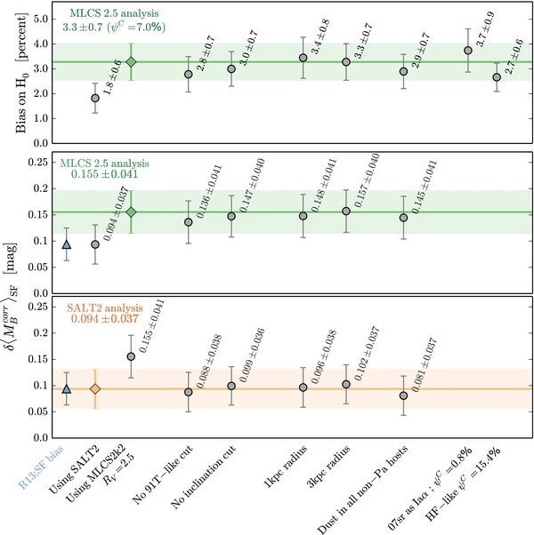
Figure 2. Summary of the influence of the analysis choices made in the paper. The main analysis results are indicated in the upper left of their corresponding panels and drawn as horizontal lines. The shaded bands indicate the corresponding ±1 σ errors. Lower and Middle panels: The LSF bias as presented in Section 2, measured using Hubble residuals from H09 based on SALT2 (lower) and MLCS2k2 (middle) lightcurve parameters. Upper panel: The H0 bias, as presented in Section 3, using Hubble residuals based on MLCS2k2 lightcurve parameters, as in SH0ES11. The main H0 bias uses ψC = 7.0%, but we also present two variants. We consider the case when SN 2007sr is assumed to be a Iaα, in which case ψC = 0.8%, as well as the case where the Cepheid hosts are measured with angular resolution and signal-to-noise typical of the Hubble-flow sample, in which case ψC = 15.4%. The summary results are reported in Table 5.
Download figure:
Standard image High-resolution imageTable 3. The Local Star-formation Bias and Environmental Variations in the H09/GALEX Sample
| Light-curve fitter | Star-formation Bias | SN Hubble Residual dispersiona | ||||
|---|---|---|---|---|---|---|
| Fraction of |  |
Bias | SNe Ia | SNe Iaα | SNe Ia |
|
| SNe Ia (ψ) |
(mag) | Signifiance | (mag) | (mag) | (mag) | |
| SALT2 | 48.9% | 0.094 ± 0.037 | 2.5σ | 0.147 ± 0.019 | 0.144 ± 0.024 | 0.144 ± 0.026 |
| MLCS2k2 RV = 1.7 | 52.2% | 0.136 ± 0.040 | 3.4σ | 0.165 ± 0.011 | 0.127 ± 0.019 | 0.180 ± 0.014 |
| MLCS2k2 RV = 2.5 | 52.1% | 0.155 ± 0.041 | 3.8σ | 0.166 ± 0.012 | 0.122 ± 0.020 | 0.181 ± 0.015 |
| MLCS2k2 RV = 3.1 | 52.4% | 0.171 ± 0.040 | 4.2σ | 0.183 ± 0.011 | 0.137 ± 0.018 | 0.202 ± 0.013 |
Note. aWeighted rms with noise due to small-scale galaxy peculiar velocities (300 km s−1) removed.
Download table as: ASCIITypeset image
Finally, for use with Equation (A.14) in Appendix A of R13, which details the relation between the local star-formation bias and the host mass step, we report the fraction of high mass hosts, FH, in the H09/GALEX sample. We find FH = 89% for the H09 sample studied here, and expect it to be representative of most nearby samples currently in use. This compares with a high-mass fraction of only ∼55% for the SNfactory (Childress et al. 2013b), SDSS (Gupta et al. 2011) or PTF (Pan et al. 2014) samples.
2.4. Robustness of the H09 Local Star-formation Bias
In this section, we test the influence of the various criteria used in performing this portion of the analysis. These include the sample selection, the radius chosen to represent the local environment, and the dust correction. The effects of changing each of these selections in turn are illustrated in the lower two panels of Figure 2, and are discussed in the following paragraphs. Two key ideas to keep in mind here are that (1) while the specific values of ΣSFR can change with the details of the measurement technique, only SNe Ia near the ΣSFR threshold can have much effect, and (2) any errors made in categorizing the local environment are most likely to decrease the measured size of any real LSF bias by mixing SNe Ia from different environments.
Sample construction. In the main analysis, we made two sample selections (see Table 1). As in R13, we removed 91T-like SNe and the SNe from highly inclined host galaxies. Alterations in these selection criteria change the LSF bias by less than 0.015 mag, as illustrated in Figure 2.
Local environment measurement radius. In Section 2.2.4 we presented the rationale for our use of a 2 kpc radius aperture to define the "local" SN environments. We have tested the impact of using either a smaller (1 kpc) or larger (3 kpc) aperture, and find changes of less than 0.01 mag, regardless of which light-curve fitter Hubble residuals are used.
Dust correction. In our main analysis, when the global sSFR was not at least one standard deviation from the threshold set at −10.5 dex, an extinction correction was applied only if the FUV signal was detected at more than 2 σ in a host galaxy compatible with being SF (Section 2.2.2). Here we test the extreme case of applying dust extinction corrections to the local environment whenever the host galaxy is not globally passive. This tests the possibility that strong extinction is responsibly for pushing the observed FUV signal below the 2σ detection threshold. This test essentially consists of assigning the typical AFUV = 2.0 ± 0.6 mag found by Salim et al. (2005, 2007) to the SNe Ia from globally SF hosts that were not corrected for extinction in the main analysis. This change to the analysis reduces the amplitude of the LSF bias by only ∼0.010–0.013 mag, as shown in Figure 2.
GALEX sensitivity. We have considered whether the limited sensitivity of some GALEX exposures might affect our results. Fortunately, almost half of the hosts considered have exposures several times longer than those of the main GALEX AIS survey (see Table 2). We find no direct correspondence between SF sensitivity and redshift or classification probability in the current data set.
In summary, the measurement of the H09 LSF bias is robust at the ∼0.015 mag level against variations in the analysis.
2.5. Hubble Residual Bimodality
R13 suggested the presence of a bimodal structure in the  distribution of the SNfactory data set (see the lower-right histogram in Figure 1 of R13). The brighter mode consisted entirely of SNe Ia from locally passive environments, Ia, while the fainter mode consisted of SNe Ia from a mix of Iaα and Ia environment. While the fainter mode extended over the full range of host galaxy masses, the brighter mode was concentrated in the high-mass half of the distribution.
As in R13 we find that the SNe Ia having locally SF environments have a ∼30% tighter dispersion than the overall sample. After removing the random noise expected due to small-scale galaxy peculiar velocities, we find that the Iaα population has a weighted rms of only 0.127 ± 0.019 mag when using MLCS2k2 Hubble residuals. See Table 3 for a summary of the weighted rms for each environmental subpopulation.
We have fitted the R13 bimodal model, without any adjustment, to the environmentally categorized Hubble residuals of our H09 subset. Here we find that the R13 model is a better fit than a single Gaussian whose dispersion is allowed to float. Specifically, we measure differences of −4.6 and −0.9 in favor of the bimodal model for the Akaike information criterion corrected for finite sample size (AICc) when using MLCS2k2 and SALT2 Hubble residuals, respectively. The result using MLCS2k2 strongly favors the R13 bimodal model, but the evidence for bimodality using the H09 SALT2 Hubble residuals is weaker than found in R13. The mixed evidence for bimodality here is not surprising given the generally larger measurement uncertainties reported by H09.
2.6. Combined Local Star-formation Bias
The LSF bias measured for the H09 sample is in remarkable agreement with the value determined in R13 using the SNfactory sample, both based on SALT2 Hubble residuals. Under the assumption that the LSF bias is a universal quantity, we can combine these measurements (first averaging the six SNe Ia in common). Doing so, we find a common LSF bias of  0.094 ± 0.025 mag, which constitutes a 3.8 σ measurement of this environmental bias. Alternatively, this becomes 0.110 ± 0.024 mag when combining the R13 results with the MLCS2k2 Hubble residuals from the H09/GALEX data set.
3. CONSEQUENCE OF THE LOCAL STAR-FORMATION BIAS ON THE MEASUREMENT OF H0
In this second half of the paper, we turn to the question of whether the confirmed LSF bias affects the current measurements of H0. Currently, the most accurate method to directly measure H0 is to use SNe Ia in the Hubble flow (HF) to estimate H02〈LSN〉, and then calibrate the average standardized SN Ia luminosity, 〈LSN〉, using SNe Ia with accurate and independent distance measurements. The period–luminosity relation of a large number of Cepheid variable stars within a modest number of nearby SN Ia host galaxies has been used to provide a calibration of 〈LSN〉 (Riess et al. 2011; Freedman et al. 2012). Underlying this approach is the assumption that 〈LSN〉 is the same in both the Cepheid-calibrated and the Hubble-flow samples.
However, the Cepheid-calibrated sample targets globally young environments since Cepheids are very young stars, with ages less than 100 Myr. Indeed, the main sequence counterparts of classical Cepheids are B-type stars like those contributing to the FUV flux we use here as a star formation indicator (for a review, see Turner 1996). Thus, the fraction of SNe Ia in SF environments (Iaα) is likely to be higher for the Cepheid sample than for the Hubble flow sample. The average SN Ia standardized luminosity will then differ between the two samples due to the LSF bias demonstrated in Section 2.3; this, in turn, biases the measurement of H0. In the following sections, we estimate the amplitude of this bias on the Hubble constant.
The correction to H0, resulting in an unbiased measurement,  , can be written quite generally as:
Here ψC and ψHF respectively denote the fraction of SNe Ia in the specific Cepheid-calibrated and Hubble-flow samples being compared which have locally passive (Ia) environments. The two terms on the right-hand side work together; even if there is an LSF bias, it only biases H0 if ψC and ψHF are not equal. The appropriate values of ψ are calculated by taking the average of the  probabilities for the corresponding data sets. Conceptually, the net effect of Equation (2) is to form the weighted average of two Hubble diagrams—one for SNe Iaα and one for SNe Ia.
Assuming that the LSF bias,  , is a universal quantity, it may be determined from the specific sample under study or by including external measurements. Note that the value of ψ for any external sample used solely to measure
  is immaterial in this context. At most it affects the sensitivity of the
  measurement from the external sample; it does not enter into ψHF. Conversely, if there are SNe Ia used to calculate both the original H0 measurement and
  , as is the case here, there will be positively correlated errors between these two quantities.
Having established the value of  in Section 2.3, we now evaluate the other inputs to Equation (2), the fraction of SNe Ia with locally passive environments in the Hubble flow and Cepheid-calibrated SN Ia host galaxies. Because the main analysis in SH0ES11 used MLCS2k2 RV = 2.5 Hubble residuals, we do so here.
3.1. The Fraction of Ia Among the SH0ES11 Cepheid Galaxies
We first examine the eight SNe Ia hosts whose distances were measured using the Cepheid period–luminosity relation by SH0ES11. We measure their  in the same manner as for the H09 sample, as described in Section 2.1. The results are summarized in Table 4. The top half of the table summarizes the galaxies used by SH0ES11 to measure H0, while the bottom half presents our measurements for additional SN Ia host galaxies whose Cepheid-based distances are anticipated. The local environments for seven of the eight are covered by both GALEX FUV and NUV observations, while SN 1998eq lacks FUV coverage.
Table 4. Local UV Environments of the Cepheid–SNe Ia Sample
| Name | FUV | NUV | AFUV | Host | Dust | log (ΣSFR) |  |
|---|---|---|---|---|---|---|---|
| (mag) | (mag) | (mag) | Type | Corr. | (M☉ kpc−2 yr−1) | (percent) | |
| SN1981B | 17.34 ± 0.02 | 16.91 ± 0.01 | 1.7 ± 0.1 | SF | Y | −2.34 ± 0.02 | 0 |
| SN1990N | 18.76 ± 0.10 | 18.46 ± 0.04 | 1.5 ± 0.3 | SF | Y | −2.67 ± 0.13 | 9 |
| SN1994ae | 18.33 ± 0.08 | 17.77 ± 0.04 | 2.1 ± 0.3 | SF | Y | −2.09 ± 0.11 | 0 |
| SN1995al | 16.49 ± 0.03 | 15.87 ± 0.01 | 2.3 ± 0.1 | SF | Y | −1.44 ± 0.03 | 0 |
| SN1998aq | no image | 16.29 ± 0.00 | ⋅⋅⋅ | SF | ⋅⋅⋅ | > − 2.4a | 0 |
| SN2002fk | 16.46 ± 0.01 | 15.87 ± 0.00 | 2.2 ± 0.0 | SF | Y | −1.09 ± 0.01 | 0 |
| SN2007af | 17.67 ± 0.02 | 17.27 ± 0.01 | 1.6 ± 0.1 | SF | Y | −2.18 ± 0.03 | 0 |
| SN2007sr b | 22.08 ± 0.57 | 20.65 ± 0.13 | 2.3 ± 0.6 | SF | Y | −3.68 ± 0.33 | 50 c |
| SN2001el | 16.85 ± 0.03 | 16.41 ± 0.01 | 1.7 ± 0.1 | SF | Y | −1.98 ± 0.04 | 0 |
| SN2003du | 18.66 ± 0.10 | 18.44 ± 0.04 | 1.3 ± 0.3 | SF | Y | −2.29 ± 0.11 | 0 |
| SN2005cf b | 22.29 ± 0.25 | 21.16 ± 0.06 | 2.8 ± 0.5 | SF | Y | −3.34 ± 0.23 | 100 |
| SN2011fe | 14.95 ± 0.01 | 14.62 ± 0.01 | 1.3 ± 0.1 | SF | Y | −2.26 ± 0.02 | 0 |
| SN2012cg | 16.67 ± 0.01 | 15.91 ± 0.00 | 2.7 ± 0.1 | SF | Y | −1.62 ± 0.01 | 0 |
| SN2012fr | 17.54 ± 0.01 | 17.02 ± 0.00 | 2.0 ± 0.1 | SF | Y | −2.15 ± 0.02 | 0 |
| SN2012ht | 20.42 ± 0.04 | 19.68 ± 0.01 | 2.7 ± 0.1 | SF | Y | −2.20 ± 0.05 | 0 |
| SN2013dy | 15.64 ± 0.00 | 15.31 ± 0.00 | 1.4 ± 0.1 | SF | Y | −1.87 ± 0.00 | 0 |
Notes.
aBased on NUV magnitude, assuming FUV-NUV = 1 and AFUV = 0.
bTails of interacting galaxies,  could be problematic.
cSee Section 3.1.
could be problematic.
cSee Section 3.1.
Download table as: ASCIITypeset image
Table 5. Effect of SN Ia Environmental Bias on H0
| Component | SALT2 | MLCS2k2 | ||
|---|---|---|---|---|
| RV = 1.7 | RV = 2.5 | RV = 3.1 | ||
| Host-mass correctiona | +0.75% | |||
| LSF-bias correction | −1.8% ± 0.6% | −2.9% ± 0.7% | −3.3% ± 0.7% | −3.6% ± 0.7% |
| Net bias | −1.1% ± 0.6% | −2.1% ± 0.7% | −2.6% ± 0.7% | −2.9% ± 0.7% |
Note. aRemoval of the host-mass corrections applied by SH0ES11 (see their Section 3.1) since the LSF bias already accounts for the host-mass bias. We assume that the bias used for MLCS2K2 was also used for the SALT analysis.
Download table as: ASCIITypeset image
Although SN 1998aq does not have FUV imaging, it does have a strong NUV signal. We can use the NUV signal along with very conservative assumptions to categorize the local environment of SN 1998eq as SF. Specifically, even assuming an extreme UV color of FUV−NUV =1 (see Figure 13 of Salim et al. 2007) and no dust extinction still requires a minimum value for the local star formation density of log (ΣSFR) > −2.46 dex.
SN 2007sr is an exceptional case, as it is located in the well-known tidal tail of the merging galaxies NGC 4038/39 (the Antennae). Tidal environments are known as sites of strong star formation (e.g., Neff et al. 2005; Smith et al. 2010; Kaviraj et al. 2012). The Antennae tidal tail is indeed quite blue (Hibbard et al. 2005), and contains star clusters with mean ages of 10–100 Myr (Whitmore et al. 1999; Fall et al. 2005). Therefore, one might presume that SN 2007sr should be classified as a Iaα. However, SN 2007sr actually lies at a projected separation of 2 kpc from the spine of the tidal tail, and Hibbard et al. (2005) estimate an age around 400 Myr along the portion of the tail projected closest to SN 2007sr. (Note that the Hibbard et al. 2005 age determinations did not include correction for possible dust extinction, and so may be too large.) An age of 400 Myr is older than the estimated dynamical time for the tidal tail, and would therefore suggest that stars near the location of SN 2007sr were originally formed in the disk of their parent galaxy. Tidal forces will act in a similar manner on the volume of stars originally local to the SN 2007sr progenitor, but it is likely that the stars are now more spread out due to dynamical evolution, having moved SN 2007sr off the spine of the tail and lowering the stellar surface density, and thus the measured ΣSFR, compared to the original environment.
When faced with such ambiguity for the Hubble-flow sample, as with highly inclined host galaxies, the simplest avenue was to cut them from the sample. Doing that in this case would result in a value ψC ∼ 0, along with a slight increase in the uncertainty on H0 due to the smaller number of calibrators, since all the remaining environments for the Cepheid-calibrated SNe Ia are SF. Given the possibility that SN 2007sr may be slightly too old to be counted as Iaα, this choice could slightly overestimate the final correction to H0 that is needed. To better reflect the ambiguity for this calibrator, we will take a neutral value of  for our main analysis. We note that SN 2005cf, listed in Table 4 as a likely future calibrator, is also located in a tidal tail. Thus, the question of the proper categorization of tidal tails will resurface when it is time to incorporate SN 2005cf into the measurement of H0.
Combining the eight individual  , we find ψC = 7.0% as the fraction of SNe Ia in the Cepheid-calibrated SNe Ia used for the SH0ES11 measurement of the local Hubble constant. As anticipated, the local environments of this sample is predominately SF.
3.2. The Fraction of Ia in our H09/GALEX Hubble-flow Sample
If we had estimates of  for all 140 nearby Hubble-flow SNe Ia used by SH0ES11 we could calculate and apply the resulting ψHF directly in Equation (2). However, ∼30 of the Hubble-flow SNe Ia used by SH0ES11 are not contained in H09, and in addition, we do not have
  estimates for another 30 due to insufficient GALEX coverage or selection cuts (see Table 1). Thus, unlike the above estimate of ψC, our estimate of ψHF will need to be statistical.
The fact that we still have ∼60% of the SNe Ia in common will reduce the uncertainty substantially since we incur a statistical error (beyond that already incorporated in the  values for individual SNe) only for the ∼40% that remain unmeasured. We have shown in Section 2.1 that the H09/GALEX data set is statistically representative of the entire H09 sample, and we expect that to be true for the ∼30 SH0ES11 Hubble-flow SNe Ia not in H09.
For the H09/GALEX subset having MLCS2K2 measurements we find ψHF = 52.1%. For those with SALT2 measurements ψHF = 48.9%. This is in agreement with the value ψHF = 50.0% ± 5.3% in R13. More comparable is the subset of high-mass hosts in R13, for which the value is slightly higher, ψHF = 63.4% ± 7.5%. This may reflect differences between the untargeted SNfactory search that provided the most SNe Ia in R13 and galaxy-magnitude-limited searches that provided most of the SNe Ia in H09. It also could be due to a greater chance of false-positive associations due to the 4 × greater area covered by the larger aperture used here. Applying ψHF = 52.1% as a statistical estimator to the 59 SH0ES11 SNe Ia environments we were unable to measure, and combining with those we have measured, gives ψHF = 52.1% ± 2.3%. The variations due to the alternatives explored in Section 2.4 are within the final statistical uncertainty on ψHF for the SH0ES11 Hubble-flow sample, and are reflected in the calculations of the variations shown in Figure 2.
3.3. Hubble Constant Corrected for the Local Star-formation Bias
As a result of the high fraction of local SF environments for the SNe Ia in the SH0ES11 sample, they do not provide a calibration that is representative of the H09 nearby Hubble-flow sample. In Section 3.4 we will present further insights into, and explore the robustness of this measured difference in the values of ψHR and ψC.
Using Equation (2) with values ψHF = 52.1% ± 2.3%, ψC = 7.0%, and  0.155 ± 0.041 mag we estimate that the Hubble constant is currently overestimated by 3.3% ± 0.7% due to the LSF bias. As will be discussed in Section 3.5, a small fraction of this bias most likely has been taken into account already because SH0ES11 applied a 0.75% correction to account for potential host-mass dependency in the SN standardized magnitudes. Since the correction for the local star-formation bias also corrects for the host-mass effect (see Section 3.5), we estimate an effective correction to H0 of −2.6% ± 0.7% (see Table 5).
There have been several updates to the basic ingredients since the SH0ES11 analysis. Humphreys et al. (2013) reported an improved value for the distance to the NGC 4258 megamaser that served as one of the zero points for the Cepheid distance scale (along with the LMC distance and parallaxes for Milky Way Cepheids). Efstathiou (2014) re-examined the selection of Cepheids and the resulting calibration of the Cepheid period–luminosity relation for the SN host galaxies, slightly modifying those distances. Since it is the most recent, and includes the revised distance to NGC 4258, we will use the Efstathiou (2014) analysis as our baseline in quantifying how the LSF bias affects the apparent tension between direct and indirect measurements of H0. Note that correction for the LSF bias involves a change to the luminosities assigned to SNe Ia in the Hubble flow relative to those in the Cepheid sample; we make no adjustments to the distances assigned to the Cepheid-calibrated SN Ia host galaxies.
By applying Equation (2), we calculate a value of the Hubble constant corrected for the LSF bias of  = 70.6 ± 2.6 km s−1 Mpc−1 when using the LMC distance, Milky Way parallaxes, and the NGC 4258 megamaser as the Cepheid zero point as in SH0ES11 and Efstathiou (2014). If the NGC 4258 megamaser is used as the sole zero point of the Cepheid distances and the new Humphreys et al. (2013) distance is used with the Efstathiou (2014) analysis, the revised H0 is lower, but less certain, at 68.8 ± 3.3 km s−1 Mpc−1. Table 6 summarizes the LSF-bias corrections for both the SH0ES11 and Efstathiou (2014) estimations of H0, when using either the megamaser or the three Cepheid anchor(s). Details of the contributions to each correction are given, along with the new level of agreement with several recent indirect CMB-based measurements of H0. We emphasize that the SH0ES11 analysis and our corrections both use MLCS2k2 with RV = 2.5, and thus are fully consistent with regard to choice of lightcurve fitter. Our revised H0 is now compatible at the 1σ level with these indirect measurement of the Hubble constant for a flat ΛCDM cosmology.
Table 6. Direct Measurement of the Hubble Constant (in km s−1 Mpc−1)
| Riess et al. (2011) | Efstathiou (2014) | |
|---|---|---|
| anchors: NGC 4258, milky way parallaxes, and lmc distance | ||
| Starting H0 | 72.7 ± 2.4a | 72.5 ± 2.5 |
| No mass bias correction | +0.5 | +0.5 |
| LSF-bias correctionc | −2.4 ± 0.5 | −2.4 ± 0.5 |
| Revised H0 | 70.8 ± 2.5 | 70.6 ± 2.6 |
| New CMB tensiond | 1.3σ/0.6σ/1.1σ | 1.2σ/0.5σ/1.0σ |
| anchor: NGC 4258 | ||
| Starting H0 | 72.0 ± 3.0b | 70.6 ± 3.3 |
| No mass bias correction | +0.5 | +0.5 |
| LSF-bias correctionc | −2.4 ± 0.5 | −2.3 ± 0.5 |
| Revised H0 | 70.2 ± 3.0 | 68.8 ± 3.3 |
| New CMB tensiond | 0.9σ/0.3σ/0.7σ | 0.5σ/0.2σ/0.2σ |
Notes. Top: using Cepheid distances calibrated to the megamaser NGC 4258, Milky Way parallaxes, and LMC distance. Bottom: using Cepheid distances calibrated solely with the distance to the NGC 4258 megamaser. aAfter including the recalibration of NGC 4258 (−1.1 km s−1 Mpc−1; Humphreys et al. 2013) and using the prescription given in Section 3.1 of SH0ES11. bFrom Humphreys et al. (2013). cAdd an extra −0.3 km s−1 Mpc−1 if SN2007sr is considered to be Iaα. dTensions with Planck (67.3 ± 1.2 km s−1 Mpc−1; Planck Collaboration et al. 2014), WMAP 9-year (69.32 ± 0.80 km s−1 Mpc−1; Bennett et al. 2013; Hinshaw et al. 2013), and revised Planck (68.0 ± 1.1 km s−1 Mpc−1; Spergel et al. 2013), respectively.
Download table as: ASCIITypeset image
We note that this estimate can be improved in the future by the various teams who employ SNe Ia to measure H0, by improved matching of the local SN environments between the calibrator and Hubble-flow samples.
3.4. Robustness of the H0 Correction
The robustness of our correction to H0 depends on the robustness of the inputs to Equation (2). In Section 2.4 we have already explored the robustness of the local star-formation bias to changes in our sample selection and measurement procedures. The other key ingredient for the bias on H0 is the difference in the values of ψHF and ψC. In the upper panel of Figure 2, we show how these analysis parameters affect the measurement of the H0 bias (see Section 2.4). None have a significant impact.
SN 2007sr classification.
To further explore the difference between ψHF and ψC we consider the case where SN 2007sr is Iaα. This increases the LSF bias on H0 by 0.4%; hence if one considers this a false-negative due to tidal dilution of the local star-formation surface density, then an extra −0.3 km s−1 Mpc−1 should be applied to the aforementioned revised H0 values. The signs of these changes reverse if SN 2007sr is instead considered Ia. These changes are within our quoted uncertainty.
Simulation of distance effects.
We next considered possible effects due to the redshift difference between the two samples by simulating what value of ψC would have resulted if the Cepheid-calibrated hosts had been observed with the same distances and exposures as the H09 Hubble-flow sample. For each of the six Iaα Cepheid-calibrated hosts having direct FUV detections, the star-formation surface densities were measured using the full set of procedures described in Section 2 after degrading the spatial resolution and increasing the noise to match each of the Hubble-flow galaxies. The net effect, averaged over all pairings, was to increase ψC to 15.4%. This was primarily due to changes in  for the host of SN 1990N when simulated at higher redshift or with shorter GALEX exposure. The resulting change in the H0 bias is once again well within the quoted uncertainties. This is due in part to the fact that we are already accounting for noise by using the full
  probability distribution functions.
Chance of low ψC.
One might expect the Cepheid-calibrated sample to reflect the Ia fraction of 24.9% found for globally SF galaxies (as defined in Section 2.2.2) in the Hubble-flow sample. In fact the Ia fractions are consistent; application of Fisher's Exact Test20, applicable to two sets of categorical data, as here, gives a 18% chance of finding no locally passive environments for the SH0ES11 sample.
Good consistency is also found when comparing based solely on morphology. The SNe Ia hosts with Cepheid calibration have Hubble types Sb—Sm. In our Hubble-flow sample we find that for SN host galaxies of these types the passive fraction is ∼26%. Application of Fisher's Exact Test for this case shows that the passive fraction in the Hubble-flow and current Cepheid-calibrated samples have a 17% probability of being the same. Even including the low locally passive fraction for the Cepheid-calibrated SNe expected to be used in the future (see Table 4), the probability of a common locally passive fraction is 14%.
Consistent, low  dispersions.
One final indicator that the SNe Ia in Cepheid hosts are of class Iaα is that they share the small dispersion that R13 found for this subclass. Using Table 3 of SH0ES11 we calculated an unbiased weighted dispersion in Cepheid-calibrated standardized SN Ia absolute magnitudes of only 0.123 ± 0.034 mag. After removing the dispersion due to Cepheid distance measurement errors, the SN Ia dispersion drops to only 0.101 mag. This agrees well with the dispersion of 0.099 ± 0.009 mag found by R13 for their SNe Ia associated with SF environments, and with the 0.122 ± 0.020 mag dispersion of the Iaα in the H09 Hubble-flow sample (see Table 3). The small dispersion of the Cepheid-calibrated SNe Ia and its similarity to the dispersion of the R13 and H09 Iaα subsets could be a coincidence, but as the overall sample dispersion is much larger, 0.166 ± 0.012 mag, the likelihood ratio strongly favors our result that these SNe Ia truly belong to the Iaα category.
dispersions.
One final indicator that the SNe Ia in Cepheid hosts are of class Iaα is that they share the small dispersion that R13 found for this subclass. Using Table 3 of SH0ES11 we calculated an unbiased weighted dispersion in Cepheid-calibrated standardized SN Ia absolute magnitudes of only 0.123 ± 0.034 mag. After removing the dispersion due to Cepheid distance measurement errors, the SN Ia dispersion drops to only 0.101 mag. This agrees well with the dispersion of 0.099 ± 0.009 mag found by R13 for their SNe Ia associated with SF environments, and with the 0.122 ± 0.020 mag dispersion of the Iaα in the H09 Hubble-flow sample (see Table 3). The small dispersion of the Cepheid-calibrated SNe Ia and its similarity to the dispersion of the R13 and H09 Iaα subsets could be a coincidence, but as the overall sample dispersion is much larger, 0.166 ± 0.012 mag, the likelihood ratio strongly favors our result that these SNe Ia truly belong to the Iaα category.
3.5. Connection to the Host Mass Step Bias Correction
SH0ES11 argued that the step in Hubble residuals occurring around a host mass of 1010 M☉ has a small impact on their estimation of H0 since the host masses for the Cepheid-calibrated SNe Ia are similar to those of the Hubble-flow SNe Ia from H09. Using a linear correction of Hubble residual versus host mass based on external information, the SH0ES11 estimate for H0 is reduced by only 0.75% (see their Section 3).
Here we have shown that even for a sample such as that of H09 where almost all hosts are on the high-mass side of the mass step, there is a bias that is just as large as past studies have found for the size of the host-mass correction over the full mass range of SN Ia host galaxies (e.g., Childress et al. 2013a). These results and those of R13 indicate that star formation is a more important driver than host mass, and that in fact, the host-mass step may simply be a projection of the local star-formation bias in combination with the rapid change in the fraction of SF galaxies as a function of mass as in Figure 11 of Childress et al. (2013a).
If the LSF bias is indeed the more deep-rooted cause of the mass step, then correcting for the LSF bias naturally corrects for the host-mass dependency (see also Appendix A of R13). The H09 sample was used by Kelly et al. (2010) to originally discover the SN Ia host mass bias; for our subset—having significant overlap with that of Kelly et al. (2010)—we find that the mass step calculated at their division point of 1010.8 M☉ drops from 0.100 ± 0.040 mag before correction for the LSF bias to 0.026 ± 0.039 mag afterward. This demonstrates that the LSF bias does in fact remove the mass step. Consequently, for our analysis to be self-consistent we remove the 0.75% offset to H0 applied by SH0ES11, where the intent was to account for the host-mass effect, since our LSF bias correction has removed it from the data.
4. CONCLUSION
We have used the nearby SNe Ia from the independent Constitution data set compiled by H09 to confirm the local environment bias in SNe Ia standardized magnitudes first seen by R13 in the Nearby Supernova Factory SN Ia sample. Using Hubble residuals as presented by H09 along with our GALEX-based measurements of the local star formation, we confirm this bias for standardization using either SALT2 or MLCS2k2 lightcurve parameters with  0.094 ± 0.037 mag and
  0.155 ± 0.041 mag, respectively. Whereas R13 used Hα as star formation indicator, here we use the FUV flux as measured by GALEX. Together these results demonstrate that the effect is not particular to the sample, lightcurve standardization, or type of star formation indicator that is used.
Combining our new SALT2 bias measurement with that from R13 we find that SNe Ia from locally SF environments are  0.094 ± 0.025 mag fainter after standardization than those from locally passive environments. This constitutes a 3.8 σ measurement of this environmental bias. We also measure that in nearby SN Ia samples dominated by high-mass host galaxies, such as that drawn from Constitution, typically ∼50% of the SNe Ia arise in locally passive environments.
This local star-formation bias has a direct consequence on the precision measurement of H0, as exemplified by the SH0ES11 program. We find the local environments of SNe Ia whose absolute magnitudes were calibrated by SH0ES11 using the Cepheid period–luminosity relation are overwhelmingly SF. This in itself is not surprising because Cepheids are young stars. However, in the presence of a local star-formation bias, it means that the standardized magnitudes of these SNe Ia will be dimmer on average than those of the Hubble-flow comparison sample. By applying our measurements of the amplitude of the local star-formation bias along with the relative fractions of SNe Ia in SF or passive local environments for each of the Cepheid-calibrated and Hubble-flow samples, we find that a 3.3% ± 0.7% correction (−2.4 ± 0.5 km s−1 Mpc−1) to the SH0ES11 measurement of H0 is required. The final corrected value, including the revised NGC 4258 megamaser distance (Humphreys et al. 2013), the refined Cepheid analysis of Efstathiou (2014), and backing out the small host-mass correction implemented in SH0ES11, becomes H0 = 70.6 ± 2.6 km s−1 Mpc−1 when starting from the main SH0ES11 analysis using MLCS2k2 SN lightcurve parameters. This corrected value for the Hubble constant is within 1 σ of the current CMB indirect estimations of the Hubble constant from Planck (Planck Collaboration et al. 2014; Spergel et al. 2013) and Wilkinson Microwave Anisotropy Probe (Bennett et al. 2013; Hinshaw et al. 2013). We note that while our corrected value for H0 lies within the uncertainties quoted by SH0ES11, it is a ∼5 × larger correction than their quoted uncertainty on the zero point from SNe Ia in the Hubble flow.
Looking forward to future studies to measure H0, we present star-formation measurements for additional nearby SNe Ia whose distances may soon be calibrated using the Cepheid period–luminosity relation. These are also locally SF, and so the star-formation bias will need to be taken into account in future analyses. Further, we note that similar caution is necessary when using SNe Ia with other distance indicators, such as the Tully Fisher relation, surface brightness fluctuations and tip of the red giant branch, which target galaxies where star formation is unusually high or low.
We also note the discovery of new star formation at SN Ia sites in several morphological E/S0 galaxies; such cases may lead to a better understanding of the connection between different star formation histories and the properties of SNe Ia.
We thank Jake Simones, Evan Skillman, Adam Riess, Robert Kirshner, and Saurahb Jha for useful discussions. This work is based on observations made with the NASA Galaxy Evolution Explorer. GALEX is operated for NASA by the California Institute of Technology under NASA contract NAS5-98034. This work was supported in part by the Director, Office of Science, Office of High Energy Physics, of the U.S. Department of Energy under Contract No. DE-AC02- 05CH11231; in Germany by the DFG through TRR33 "The Dark Universe"; in France by support from CNRS/IN2P3, CNRS/INSU, and PNC; and in China from Tsinghua University 985 grant and NSFC grant No. 11173017. LPNHE acknowledges support from LABEX ILP, supported by French state funds managed by the ANR within the Investissements d'Avenir programme under reference ANR-11-IDEX-0004-02. NC is grateful to the LABEX Lyon Institute of Origins (ANR-10-LABX-0066) of the Université de Lyon for its financial support within the program "Investissements d'Avenir" (ANR-11-IDEX-0007) of the French government operated by the National Research Agency (ANR). This research has made use of the NASA/IPAC Extragalactic Database (NED), which is operated by the Jet Propulsion Laboratory, California Institute of Technology, under contract with the National Aeronautics and Space Administration. Some of the data presented in this paper were obtained from the Mikulski Archive for Space Telescopes (MAST). STScI is operated by the Association of Universities for Research in Astronomy, Inc., under NASA contract NAS5-26555. Support for MAST for non-HST data is provided by the NASA Office of Space Science via grant NNX13AC07G and by other grants and contracts.
APPENDIX A: ILLUSTRATION OF MLCS2K2-BASED HUBBLE RESIDUALS
The characteristics of the Iaα and Ia SN Ia subsets shown in Figure 1 used Hubble residuals derived using lightcurve fit parameters determined using SALT2. In Figure 3 we present the analogous results using Hubble residuals based on MLCS2k2 lightcurve fit parameters.
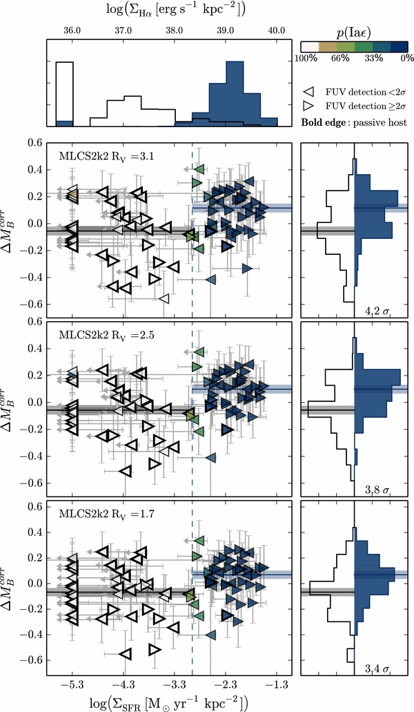
Figure 3. SN Ia MLCS2k2 standardized Hubble residuals ( ) as a function of log (ΣSFR), from the bottom to the top: RV of 1.7, 2.5, and 3.1, respectively. This plot is constructed like Figure 1.
Download figure:
Standard image High-resolution imageAPPENDIX B: R13 SAMPLE CUTS
B.1. Potential Super-Chandrasekhar SNe
In Scalzo et al. (2012), we suggested that 91T-like SNe Ia are good candidates for having masses above the Chandrasekhar limit, and demonstrated that some indeed do. Because of the possibility that these might result from a different progenitor channel, they were not considered in R13. Scalzo et al. (2012) determined the rate of pure 91T-like SNe Ia—excluding those similar to the less extreme 99aa-like subclass—to be  % of a total SN rate for a volume-limited sample. Thus, we expect 91T-like SNe Ia to be a minor component of the H09 sample. Blondin et al. (2012) have spectroscopically classified most SNe Ia in the H09 sample, however, they did not distinguish between 91T-like and 99aa-like events. Silverman et al. (2012) present spectroscopic classifications for a large sample of nearby SNe Ia having significant overlap with the H09 sample, and they do distinguish between 91T-like and 99aa-like events. Combining those studies, we therefore exclude SN 1998ab and SN 2003hu from our baseline analysis on the basis of their 91T-like character. SN 1999gp is also 91T-like, but has no GALEX data or MLCS2k2 measurement. The resulting 91T-like fraction of 2.7% matches the result of Scalzo et al. (2012). Therefore, in this regard the parent population of the SNe Ia sample studied here is in agreement with that of R13.
B.2. Highly Inclined SN Host Galaxies
In R13, highly inclined galaxies were identified as cases where a locally passive environment might incorrectly be associated with an Hα signal due to projection. In the present case, however, highly inclined galaxies are as likely to suffer suppressed FUV emission due to strong dust absorption (see, e.g., Conroy et al. 2010). Thus, it is unclear whether inclination is more likely to produce false-positive or false-negative environment categorizations.
Within the set of host galaxies studied here, SN 1992ag, SN 1995ac, SN 1997dg, SN 2006ak, and SN 2006cc are highly inclined and are classified as Iaα, and therefore may be examples where a locally passive environment has been miscategorized as a SF environment due to projection. On the other hand, SN 1998eg and SN 2006gj are examples of SNe Ia in edge-on galaxies with no FUV signal, which might be suppressed due to dust extinction. Following R13, these cases are removed from our main analysis. In Section 2.4 we examined whether including them in the main sample has any effect on our results, and found it did not. We note that such edge-on galaxies would not be suitable for Cepheid measurements either.
APPENDIX C: ADDITIONAL POTENTIAL CASES OF MISCATEGORIZATION
C.1. Bright Elliptical Cores
Another type of miscategorization can occur when the FUV signal does not directly trace star formation, namely when the signal originating from the very inner cores of E/S0 galaxies surpasses our chosen threshold simply due to the large column of stars along our line of sight (e.g., see FUV surface brightness profiles for E/S0 galaxies in Marino et al. 2011). While this problem is far worse in the NUV band, we considered it prudent to examine this in FUV as well. SNe Ia are rarely detected on E/S0 galaxy cores due to low contrast, subtraction errors, and the overall small fraction of stars projected onto the core relative to the entire galaxy, so only a dozen cases needed this special attention.
We identified two cases of SNe close to the core of E/S0 galaxies for which the GALEX FUV signal is above our threshold: SN 2005hc and SN 2005mc. These have sSFR measurements (Neill et al. 2009) that are ambiguous. In the case of SN 2005hc, there is an apparent SF disk present, which in optical light is hidden by the glare of old stars, and the SN is projected onto this disk. Therefore, the categorization of the local environment of SN 2005hc as Iaα seems correct. We note that in this case a categorization based on morphology alone—which is commonly applied in SN host studies—would produce erroneous results.
In the case of SN 2005mc, located in the (R')SB0 galaxy UGC 4414 (de Vaucouleurs et al. 1991), there is FUV light at the very core, as well as FUV light from a known SF ring. The SN lies close to the core, which is slightly bluer in FUV−NUV than the cores of normal E/S0 galaxies but not as blue as the SF ring. The SDSS spectrum of the core reveals evidence for LINER activity, with stellar-absorption-corrected Hα emission significantly weaker than [N ii] λ6583 Å or [S ii] λ6717, 6731 Å (Baldwin et al. 1981; Veilleux & Osterbrock 1987; Kewley et al. 2006). Thus, the signal in the core may be due in part to the high column density of old stars projected onto the core combined with LINER activity. To test this we remeasured the FUV flux in a 1 kpc aperture, which safely clears any light from the core. The resulting ΣSFR did not change significantly, therefore, we retain classification of SN 2005mc as having a Iaα environment.
As part of this study we examined SN 2003ic, which has an elliptical host galaxy but where GALEX shows signs of recent star-formation. It's observed ΣSFR, which was not corrected for extinction since the host appeared to be globally passive, is below our threshold and gives  . If an extinction correction had been applied, its ΣSFR would have been slightly above our threshold, with
  . It is thus likely to be the third case of an SN Ia associated with comparatively recent star-formation hidden in an otherwise normal-looking elliptical host galaxy. Förster & Schawinski (2008) and Schawinski (2009) have also searched for such cases. This SN Ia is discussed extensively in Kelly et al. (2010) since it is in the largest host galaxy in their sample and thus helps drive some of the trends they report.
C.2. Diluted FUV Signal from Star-forming Environments
Here we consider the possibility that an actively SF environment may fall below our threshold due low stellar surface density or due to geometrical dilution. Potential examples of these situations may include low surface brightness galaxies, tidal tails, dwarf galaxies, or an aperture extending beyond the nominal edge of the SN host galaxy.
Because the vast majority of SNe Ia in the H09 sample came from searches that targeted galaxies selected from magnitude-limited catalogs, the sample contains few dwarf galaxies and no known SNe Ia in tidal tails or giant low surface brightness galaxies. Nor is the drop in surface brightness with galactocentric radius a major consideration for the galaxies considered here; inspection of the GALEX Ultraviolet Atlas of Nearby Galaxies (Gil de Paz et al. 2007) shows that for galaxies typical of those hosting SNe Ia in the H09 sample, when there is active SF it rises above our SF surface density threshold over most of the face of the galaxy. Indeed, within the canonical D25 optical diameter (de Vaucouleurs et al. 1991), the azimuthally averaged FUV surface brightness range is typically only around ∼1 dex (Gil de Paz et al. 2007). Much of this variation is due to the change in filling fraction with radius rather than change in local surface brightness. This compares with the 3–4 dex amplitude of the FUV surface density signal.
However, we have identified the hosts of SN 1999aw and SN 2006an as dwarf galaxies whose sizes are smaller than the GALEX PSF. They were both found in large-area surveys unbiased toward SNe Ia in known galaxies. We estimate colors of B − V ∼ 0.4 ± 0.3 for the hosts of SN 1999aw and SN 2006an, based on photometry from Strolger et al. (2002) and SDSS, respectively. While these optical colors are not nearly as blue as those of the 125 Myr old host of SN 2007if (Childress et al. 2011), the colors for the hosts of SN 1999aw and SN 2006an are consistent with those of the blue compact dwarfs presented in Hunter et al. (2010), all of would have high star formation surface densities given FUV observations of comparable resolution and sensitivity.
In SDSS, the host of SN 2006an has a Petrosian radius of 2.4 ± 0.5 arcsec, or 1.6 ± 0.3 kpc at its redshift of z = 0.065. Thus, the effect of geometrical dilution should be small. Still, because its size is comparable to the GALEX PSF, it will be suppressed by as much as 0.3 dex since our aperture will not encompass all of the flux of a compact SF region close to SN 2006an. Thus, our current limit of log (ΣSFR) < −2.2 dex could increase to as much as log (ΣSFR) < −1.9 dex.
Strolger et al. (2002) find that the host of SN 1999aw is barely spatially resolved, having FWHM ∼ 0.4 arcsec, or ∼0.1 kpc at its redshift z = 0.038. Thus the geometrical dilution would be ∼0.6 dex for a 2 kpc radius aperture relative to the 1 kpc aperture used in R13. Measurement of the FUV flux from the host of SN 1999aw also will be suppressed by roughly 0.3 dex because our aperture doesn't cover the full PSF and the galaxy is unresolved by GALEX. Combining both effects, our current limit of log (ΣSFR) < −3.5 dex could increase to roughly log (ΣSFR) < −2.6 dex. However, if the area over which to measure SF were limited to the size of this tiny galaxy, that would raise the limit to something more like log (ΣSFR) < −0.5 dex.
For both dwarfs, much deeper FUV data would be needed in order to turn our current upper limits into detections able to firmly classify these two dwarfs. Since the current analysis has only two such cases, their impact is negligible. However, this may become an issue given the higher fraction of SNe Ia in dwarf galaxies now being found in large-area surveys unbiased toward known galaxies.
Besides the geometrical dilution for small galaxies, there will be cases where part of our UV measurement aperture extends beyond the nominal edge of the SN host galaxy. The region outside the host will bias ΣSFR low, though there is likely to be some compensation from inner, and often brighter, host light spread outward by the GALEX PSF. However, it is difficult to define an actual galaxy "edge,"; at UV wavelengths disks often extend 20%–40% beyond the nominal D25 optical diameter (Barnes et al. 2011). Therefore, we have not implemented any compensation for this potential bias.
APPENDIX D: DIFFUSE FUV EMISSION
In SF galaxies there is a diffuse FUV component that is comparable to the diffuse Hα observed outside H ii regions. In the case of Hα it remains uncertain whether this diffuse component arises directly from recombination in the warm interstellar medium or scattering off dust particles in the interstellar medium. Further information on the characteristics of the diffuse Hα can be found in Oey et al. (2007), Seon & Witt (2012) and references therein, and in Section 3 of R13. Seon et al. (2011) compare the diffuse Hα and FUV for the Galaxy, finding them to be highly correlated. They estimate that for high latitudes 37% of the Hα in the Galaxy is in a diffuse component on average, but with wide variation. They estimate that in the Galaxy the direct and diffuse components are comparable. Thilker et al. (2005) find that 65% of FUV surface brightness measured on a scale of 1.5 kpc arise from a diffuse component in M33. This compares with a 45% diffuse component for Hα. We have applied their procedure to a number of spiral galaxies in the GALEX Nearby Galaxy Atlas (Gil de Paz et al. 2007), but instead using a 2 kpc radius aperture (to match what we use for the SN host measurements), and find diffuse FUV fractions in the range 30%–80%. Such a diffuse component may increase the chance that an SN Ia with a passive local environment will be mistakenly characterized as a SF environment due to projection onto strong diffuse FUV emission. However, even if the diffuse FUV emission is due to scattering, it is mostly likely to be associated with regions of active star formation over the 2 kpc scale used here. Fortunately, the star formation surface density spans such a large range—1000× in this study and in R13—that these factors do not contribute much uncertainty to star formation categorizations for the majority of SNe Ia.
Footnotes
- 16

- 17
- 18
- 19
http://www.ned.ipac.caltech.edu. We found the NED coordinates for many SNe Ia from Hamuy et al. (1996) to be in error.
- 20
