


ABSTRACT
Epsilon Aurigae is a long-period eclipsing binary that likely contains an F0Ia star and a circumstellar disk enshrouding a hidden companion, assumed to be a main-sequence B star. High uncertainty in its parallax has kept the evolutionary status of the system in question and, hence, the true nature of each component. This unknown, as well as the absence of solid state spectral features in the infrared, requires an investigation of a wide parameter space by means of both analytic and Monte Carlo radiative transfer (MCRT) methods. The first MCRT models of epsilon Aurigae that include all three system components are presented here. We seek additional system parameter constraints by melding analytic approximations with MCRT outputs (e.g., dust temperatures) on a first-order level. The MCRT models investigate the effects of various parameters on the disk-edge temperatures; these include two distances, three particle size distributions, three compositions, and two disk masses, resulting in 36 independent models. Specifically, the MCRT temperatures permit analytic calculations of effective heating and cooling curves along the disk edge. These are used to calculate representative observed fluxes and corresponding temperatures. This novel application of thermal properties provides the basis for utilization of other binary systems containing disks. We find degeneracies in the model fits for the various parameter sets. However, the results show a preference for a carbon disk with particle size distributions ⩾10 μm. Additionally, a linear correlation between the MCRT noon and basal temperatures serves as a tool for effectively eliminating portions of the parameter space.
Export citation and abstract BibTeX RIS
1. INTRODUCTION
Disks are important features in many astrophysical environments. In particular, most—if not all—stars form within a circumstellar disk (Meyer et al. 2007). Deciphering the role disks play in the evolution of their host system is essential in determining past, present, and future aspects of the system (Kamp 2010). This includes properties of the newborn star, planet formation and characteristics, and the disk properties and lifetime. Additionally, the presence of disks in binary systems provides a unique means of analysis.
It was not until the most recent eclipse of epsilon Aurigae (2009–2011) that interferometric imaging showed a disk transiting the primary star (Kloppenborg et al. 2010; Stencel 2012). This, along with the progress of computational modeling in recent years, has opened up a new regime of study for the epsilon Aurigae system (hereafter  Aurigae). Monte Carlo radiative transfer (MCRT) codes, such as 2-Dust (Ueta & Meixner 2003), RADMC-3D (Dullemond & Dominik 2004), and Hyperion (Robitaille 2011), allow the user to "build" astrophysical systems in digital space. The outputs from these models include spectral energy distributions (SEDs), temperature gradients, polarization maps, and synthetic images, which can all be compared to observational results.
Aurigae is a unique—and often confounding—eclipsing binary system consisting of an F0Ia star (∼ 7750 K) and a disk-enshrouded main-sequence B star (Hoard et al. 2010). The first observation in 1821 described the system as "faint" (Fritsch 1824), and although observations have spanned nearly 200 yr, its evolutionary status has not been precisely determined. A large part of this uncertainty arises from the absence of an accurate distance. Distance estimates range from Hipparcos' stellar parallax measurement of 650 pc (Perryman et al. 1997) to <1.2 kpc, based on interstellar absorption and reddening (Guinan et al. 2012). The range in distances leads to a large range of mass ratios, defined as q = M1/M2 = MF0Ia⋆/MB⋆.
Another piece missing in the puzzle that is Aurigae is the lack of solid state infrared spectral lines identifying the dust parameters of the disk. Accurate modeling techniques of disk systems require that these parameters be known or assumed. We investigate another way to constrain the nature of the dust in the disk by analyzing thermal heating and cooling of the disk, using two of the better determined aspects of Aurigae: the disk temperatures (Hoard et al. 2012). These are 1150 ± 50 K for the noon side of the disk (the side of the disk facing the F0Ia star) and 550 ± 50 K for the midnight side (the side facing away from the F0Ia star). This provides a time-dependent measure of the disk-edge temperatures. We use these temperatures to constrain fits to model parameters.
The paper is organized as follows: Section 2 discusses the many unknown parameters present in the Aurigae system and those selected for the models in this paper; details of the radiative transfer, analytic, and combined modeling are given in Section 3; and Section 4 outlines the results, impact, and future work of this method.
2. SYSTEM PARAMETERS
The known parameters in the Aurigae system are quite limited because of the large uncertainty involved in the distance calculation; this creates a number of semiconstrained system parameters. This section describes the selection of parameters used in the present paper, chosen to be representative of Aurigae's broad parameter space. The values assumed for the present models are shown in Table 1.
Table 1. Modeling Parameters
| Parameter | Value | Unit | |||
|---|---|---|---|---|---|
| Assumed values | Scale height ratio | h0/rdisk | 0.03 | ||
| Accretion rate |  |
1 × 10⁻⁷ | M☉ yr−1 | ||
| Disk-flaring exponent | β | 1.15 | |||
| Surface density exponent | p | −1 | |||
| Gas-to-dust ratio | Mgas/Mdust | 100 | |||
| Disk mass | Mdisk | 1 M⊕, 1 M♃ | |||
| Particle size range | amin|amax | 0.001|1, 1|10, 10|100 | μm | ||
| Dependent on q | q = 0.75 | q = 1.25 | |||
| Distance | d | 740 | 952 | pc | |
| B star mass | MB⋆ | 7.69 | 12.71 | M☉ | |
| F0Ia star mass | MF0Ia⋆ | 5.77 | 15.89 | M☉ | |
| Disk outer radius | rdisk | 5.80 | 7.45 | AU | |
| Disk inner radius | rin | 1.34 | 3.43 | AU | |
| Disk thickness |  |
0.55 | 0.71 | AU | |
| Stellar separation | aTotal | 21.47 | 27.60 | AU | |
Download table as: ASCIITypeset image
2.1. Distance Dependence
From well-prescribed binary star physics and observations, Stefanik et al. (2010) determined a mass function of f = 2.51 ± 0.12 M☉. Kloppenborg (2012) and B. Kloppenborg (2013, private communication), through Bayesian statistical methods incorporating interferometric data and optical light-curves, determined angular distributions of the Aurigae system, including the F0Ia star diameter, disk radius, disk thickness, inclination, and others. However, for MCRT models, linear values must replace the angular distributions. This is done by selecting a q and solving for the remainder of the physical aspects of the system, e.g., d(q), where d is the distance. Therefore, the choice of q preselects a specific set of sizes and separations in the system.
Because there is a range of published distances, as described at the end of Section 1, we investigate two q's that span the published results: q = 0.75 and q = 1.25, which give d(0.75) = 740 pc and d(1.25) = 952 pc. These two are selected as representative values of the more probable solutions within the published distance range (650–1200 pc). The set of assumed and q-dependent parameters are listed in Table 1. The effect of these distances, combined with the subsequent parameters, is input into the MCRT code for a comparative analysis.
2.2. Disk Mass
The size of the circumstellar disk is set by the chosen q's and associated distances. The mass is constrained by the following assumptions: (1) the disk density structure assumes a disk viscosity and non-gravitation effects from a stable disk, e.g., a not-too-massive disk; and (2) the density scaling factor provides a slight constraint on the disk mass simply by how it distributes the mass—see Equation (1) for reference. For instance, if a particular model disk has a high mass content, more mass will distribute into the flare of the disk. If this same disk consisted of a lower mass, most of the mass would remain near the disk midplane and closer to the inner portion of the disk, affecting the observed thickness  and apparent disk radius, rdisk. The mass of the disk plays an important role in how the MCRT distributes emitted photons from the sources. Therefore, a soft constraint on the disk mass results from finding a balance of its mass, Mdisk, density structure, ρ(r, z), and size, which is done in the radiative transfer modeling.
Hinkle & Simon (1987) and Stencel et al. (2011) estimate H i gas densities using CO column densities and report nH ∼ 1024 cm−2. Based on nH, the disk's gas-to-dust ratio (Section 2.5), and the associated d (and hence, rdisk), the disk mass is constrained between ∼M⊕ and ∼0.1 M♃. Stencel (2012) uses the far-IR/submillimeter fluxes to estimate a disk mass ⩽6 M♃, making the disk dynamically significant in the system. If we assume the disk is in fact not dynamically significant, then this becomes a high upper limit. Therefore, total disk masses of M⊕ and M♃ are chosen for the current analysis to satisfy the range of plausible disk masses.
2.3. Disk Composition
The lack of spectral features in the infrared region—including the well-known 10 μm silicate feature, hydrocarbon (polycyclic aromatic hydrocarbon, PAH) signatures, and carbon dust features—points to a few possibilities for the Aurigae disk: (1) it does not contain any of these materials; (2) the composition inherently displays smooth-opacity curves through the infrared region; (3) the disk configuration prohibits observable emission or absorptive features; and/or (4) these materials are found in larger particles (that smooth out the identifiable features in the opacities). Specifically, choice 1 is difficult to physically explain, and as this paper presents the inaugural MCRT including all three system components (F01a star, B star, and disk), we dismiss this possibility (for further review of disk compositions, see Natta et al. 2007). Item 2 is addressed in Acke et al. (2013) as a possible explanation but does dismiss small PAHs which do not have a smooth opacity in the IR. Item 3 describes a configuration prohibitive of observing Kirchhoff's emission and absorption laws. In other words, the spectroscopic features are absent from the lack of cold or hot material in front of a hot or cold dense layer. Instead, the edge-on configuration reveals a dense, highly opaque wall of material, assumed to be a blackbody radiator. The fourth item is a typical assumption for disks (Min 2009) and has been suggested in previous publications for Aurigae (Hoard et al. 2010; Stencel et al. 2011).
Additionally, Muthumariappan & Parthasarathy (2012) argued with their radiative transfer modeling of the disk and central B5V star that the disk was composed of carbon. They explored compositions of amorphous carbon, amorphous silicate, and a combined 60/40 mix, concluding that a composition of 10–100 μm particle-sized amorphous carbon (originating from the mass loss of the carbon-rich, post-ABG F0Ia star) best fit the observations. They also showed with SED-fitting that interstellar medium (ISM) dust is not found in their modeled disk. Further explanation and investigation is needed, however, especially because Sadakane et al. (2010) found carbon and oxygen to be slightly underabundant in the F0Ia star; the F0Ia star approximates the solar abundances, suggesting that current information does not reasonably explain a F0Ia star-originated, carbon-rich disk.
We use disk compositions of silicate (in the form of Mg0.5Fe0.5SiO3), amorphous carbon, and a mixture of 60% silicate and 40% carbon for the present models (indicated, henceforth, as 60/40). Amorphous carbon displays a smooth-opacity curve at infrared wavelengths, which provides no prominent features in the infrared SED. In general, materials with smoother opacities are more likely to be found in those modeled situations (as in Acke et al. 2013). The index-of-refraction (m = n + ik) data are supplied by the laboratory astrophysics group at the Astrophysical Institute and University Observatory Jena (Jaeger et al. 1994; Dorschner et al. 1995; Jager et al. 1998).
We note the composition should have a slight dependence on distance, or the mass ratio, as described in Muthumariappan & Parthasarathy (2012). If the disk is younger, closer to a protoplanetary disk (q > 1), its composition is expected to be more like the ISM—the 60/40 mix. An older disk is more likely to have accreted material from the primary, and its composition is more stratified (q < 1). However, we investigate the composition of the disk as a distance-independent parameter to fully investigate the parameter space. Additional comments regarding this dependence are found in Section 4.1.
2.4. Dust Particle Size
We explore the basic assumptions of disk particles for the present work: spherical particles that exhibit optical properties from the Mie solution (originally published in Mie 1908) over a particle size distribution that follows the Mathis et al. (1977), MRN, prescription of n(a)∝a−3.5. We assume three separate groups of particle sizes, defined by their associated amin | amax: 0.001 μm | 1 μm, 1 μm | 10 μm, and 10 μm | 100 μm or small, medium, and large, respectively. Some particle descriptions not explored in the present paper include the following: nonspherical particles, layered particles, and size distribution mixing. The dust parameters for each size distribution were created with BHMie, a Mie theory wrapper for Hyperion based on the Bohren & Huffman (1983) prescription.
2.5. Additional Parameters
Disk Inner Radius. The disk's inner radius is unknown but has been estimated at ∼1 AU from transient He i 10,830 Å absorption during mideclipse (Stencel et al. 2011). For modeling purposes in the present paper, we simply assign the inner radius of the disk based on dust sublimation temperatures. Typical sublimation temperatures for silicate dust sits at about 1600 K (Cowley 1995), but is dependent on the material density and structure. Because the size of the disk is important in the mass distribution of ρ, a region of sublimation was found for each distance (because the stellar size, mass, and temperature change, the intrinsic luminosity also changes). The distance from the central B star to where the temperature ∼1600 K is taken as the disk's inner radius and shown in Table 1.
Gas-to-Dust Ratio. The models presented here use an assumed gas-to-dust (g/d) ratio of 100. The g/d ratio has a slight dependence on the selected distance, just as the disk composition: if the disk is young, it will have a g/d ∼100; a more evolved disk will tend toward g/d ∼1. Hoard et al. (2012) mention that the lack of strong molecular emission lines point toward a low g/d ratio in the disk. However, because the disk is not a pure, thin, debris disk, it should have g/d >1. A disk-edge temperature analysis of g/d = 10 models varies only slightly from the analysis with g/d = 100, but the overall effect of constraining parameters by the method presented here is minimal. Therefore, for the initial analysis, a gas-to-dust ratio of 100 is adopted. Additional modeling efforts will be needed to investigate the full impact of this parameter.
Disk Accretion Rate. The disk accretion rate onto the central B star is another unknown in the system. There is some evidence in the far-ultraviolet portion of the SED that accretion is occurring at the center of the disk (∼10−6 M☉ yr−1 from Pequette et al. 2011; Stencel et al. 2011). Yet these rates seem particularly high—given that young T Tauri stars show a median rate of ∼10−8 M☉ yr−1 (Hartmann et al. 1998)—and suggest the timescale of the disk would be distinctly short. Late-stage disk evolution exhibits accretion rates ∼10−10–10−9 M☉ yr−1 (Williams & Cieza 2011), which are ∼1000 times lower than the suggested Aurigae rates found in Pequette et al. (2011) and Stencel et al. (2011). Therefore, we adopt a reasonable estimate of ∼10−7 M☉ yr−1 for the present analysis (see also Castelli 1978).
Scale Height. The scale height at the disk edge, h0, is taken from analysis completed by Lissauer et al. (1996). They find h0/rdisk ≈ 3%. We adopt this value and use it as an input to the Hyperion code.
2.6. Observed Temperatures
Time-dependent SEDs created by Hoard et al. (2012) show a resolvable variation in the observed flux between ∼2 and ∼40 μm, providing evidence for an asymmetrically heated disk, as shown in Figure 1. The fitting of these blackbody curves provides a distance-independent feature of the Aurigae system, namely the disk-edge temperatures,  and
and  .
.

Figure 1. Top-down configuration of the epsilon Aurigae disk. The F0Ia star is assumed to be to the right of the disk. Four disk positions—all relative to the direct, F0Ia star-facing point—discussed in the present paper are shown in the figure: noon, dusk, midnight, and dawn. A dotted line separates the disk into its day and night sides, from which the observed temperatures,  and
and  , were obtained from this unresolved source. In other words, the observed temperatures result from the integrated portion of the disk facing toward the observer, represented by the shaded region along the outer edge of the disk. Also, modeled temperatures are defined at specific azimuth angles, λ, around the disk edge. These are defined at the single point rather than the face temperatures, which are integrated over the entire face of the disk pointing toward the observer. For reference, the dawn and dusk dashed line fall at about ±78° from noon.
Download figure:
Standard image High-resolution imageIt is important to remember that the day and night fluxes, along with their associated blackbody-fitted temperature profiles, are a compilation of the entire side of the disk facing toward the observer. In other words, the contribution of flux from the disk edge varies based on the curvature of the disk as well as the temperature of the disk at various positions around the disk edge. The thin crescents along the day and night sides of Figure 1 portray the effective amount of flux received from each portion of the disk; Section 3 goes through a detailed description of how the flux is coordinated with the output temperatures from the radiative transfer modeling.
As a corollary to the above statement, review the notation and descriptions in Figure 1 (similar to Figure 2 in Lissauer et al. 1996). The SED-fitted blackbody temperatures,  and
and  , are from Hoard et al. (2012). Disk temperatures at specific azimuthal angles will be defined as T(λ) throughout the paper. Azimuthal angles of 90° and 270° specify noon and midnight, respectively. We consider these angles, as well as λ = 0° and 180°, to be points of delineation between the day and night sides of the disk. These are significant for predicting observable temperature variations and making adjustments to the analytical fits (which will be discussed in Section 4).
3. MODELING METHODS
3.1. Radiative Transfer Modeling
The MCRT code used for this project is Hyperion, described in Robitaille (2011). It is an open-source program which provides a three-dimensional (3D) numerical environment for nonsymmetric placement of numerous luminosity sources in astrophysical systems. For instance, Aurigae requires a F0Ia star be placed at a single position outside of an axisymmetric disk hosting a B star. This allows for convenient analysis of the noon and midnight temperatures of the disk at rdisk. The asymmetric heating is observed at noon due to the presence of the F0Ia star, in the nonrotating MCRT case.
The disk's density is described by the flared, alpha-disk structure (Shakura & Sunyaev 1973; Pringle 1981; Bjorkman 1997):
where r and z are the cylindrical radius and height, respectively; ρ0 is a scaling factor dependent on disk mass and the disks' volume; r0 is a reference radius for the scale height, h(r) = h0(r/r0)β; β is the flaring factor; and α, the viscosity factor, is defined as β − p, where p is the surface density exponent (Cotera et al. 2001; Pascucci et al. 2004; Dullemond et al. 2007). Refer to Table 1 for the assumed values used in the present work.
Thirty-six models span the range of system parameters as discussed in Section 2. A representative example of the MCRT dust temperatures is shown in Figure 2. The other models are given in Figures 3–6. These figures display the temperature distribution of a single slice of half of the disk at a given azimuth. Each slice spans rin to rdisk and −zmax to +zmax (where zmax = 1 AU) in order to show the overall temperature structure of the disk. The images in Figures 3 and 4 mimic the same configuration of Figure 1, where the F0Ia star is located to the right. The B star is found to the left in Figures 3 and 4 and to the right in Figures 5 and 6. The figures now illustrate a flared slice through the disk, instead of a face-on, top-down view as is shown in Figure 1.

Figure 2. Representative example of the temperature output of the Monte Carlo radiative transfer modeling is shown here, spanning the radial (rin ⩽ r ⩽ rdisk) and height (1.0 AU = |z|) distributions of the disk. The densest region of the disk is outlined by the cooler, flared part of the disk where the density drops quickly to computational zero at the flare edge. Although the present paper uses a single, density-weighted temperature to describe the disk edge (see Section 3.1), inclusion of the entire disk temperature distribution illustrates the differences when considering only the disk and central B star, the basal distribution (a), vs. inclusion of the F0Ia star, the noon distribution (b). The edge temperature of (a) is Tbasal, or the coldest temperature at which the disk model will reach, based solely on the interior B star and accretional heating. Tnoon is the density-weighted temperature of the disk facing the F0Ia star. Therefore, the F0Ia star is taken as to the right of figure, whereas the B star sits in the middle of the two figures (both stars not shown). These are the same as Figures 5bVI and 3bVI, which correspond to a Jupiter-mass disk composed of large carbon particles set at a distance of 740 pc. Note the temperature differences within the internal portion of the disk, particularly along the midplane; this is important for particle growth and planetesimal formation.
Download figure:
Standard image High-resolution image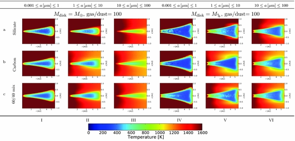
Figure 3. Radiative transfer output temperatures for the disk's noon position, with the system at d = 740 pc. Each image is a vertical slice through half of the disk, with the B star to the left and the F0Ia star to the right. The first column and last row aid as figure identifiers. The models in this figure identified as Likely in Section 4.1 are the following: aIII, aVI, bI, bV, bVI, cII, and cVI.
Download figure:
Standard image High-resolution image
Figure 4. Radiative transfer output temperatures for the disk's noon position, with the system at d = 952 pc. Each image is a vertical slice through half of the disk, with the B star to the left and the F0Ia star to the right. The first column and last row aid as figure identifiers. The models in this figure identified as Likely in Section 4.1 are the following: aVI, bI, bV, bVI, and cVI.
Download figure:
Standard image High-resolution image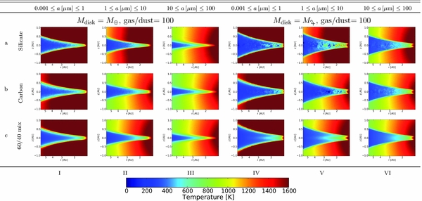
Figure 5. Radiative transfer output temperatures with the system at d = 740 pc for the basal disk. Each image is a vertical slice through half of the disk, with the B star to the right; the F0Ia star has been "turned off." The first column and last row aid as figure identifiers. The models in this figure identified as Likely in Section 4.1 are the same as Figure 3 but for the basal temperatures: aIII, aVI, bI, bV, bVI, cII, and cVI.
Download figure:
Standard image High-resolution image
Figure 6. Radiative transfer output temperatures with the system at d = 952 pc for the basal disk. Each image is a vertical slice through half of the disk with the B star to the right; the F0Ia star has been "turned off." The first column and last row aid as figure identifiers. The models in this figure identified as Likely in Section 4.1 are the same as Figure 4 but for the basal temperatures: aVI, bI, bV, bVI, and cVI.
Download figure:
Standard image High-resolution imageAdditionally, there is no F0Ia star in the Figure 2(a) plot (or those in Figures 5 and 6), as the title suggests; this is what the disk's temperature would look like without the presence of the external F0Ia star. In other words, the basal model shows the minimum temperatures the disk could have for a given set of parameters and are equivalent to those produced by Muthumariappan & Parthasarathy (2012). The basal MCRT models are effective analogues to midnight with the F0Ia star on because of the highly opaque disk. The midnight position is always the point facing away from the F0Ia star, or the side opposite noon; however, it must be noted that midnight does not always indicate basal. The MCRT modeling produces a basal temperature at midnight, but the time-dependent model described in Section 3.2 has a basal temperature toward dawn, not midnight. Again, the MCRT modeling produces midnight disk temperatures equivalent to the basal temperatures.
The images—not the MCRT models—have a temperature cap of 1600 K, which is taken as the sublimation temperature of dust particles. Some temperatures reach well beyond this maximum (toward the inner region of the disk and beyond the most dense regions of the disk), but because the observed temperatures are only 1150 and 550 K, the images' cap was assigned for readability and convenience.
Figure 2 also shows the effect of density on disk heating. The densest part of the disk is highlighted by the much cooler, flared component. The density structure is such that a steep fall-off to an effective ρ ≈ 0 occurs quickly outside of the cooler, denser region. This causes a rather immediate increase in temperature outside the disk structure. Therefore, the hot (>1600 K) regions above and below the flared disk are products of computational floating-point zero densities. Because we are most interested in the temperature at the edge of the dense disk, a density-weighted temperature average accurately portrays those temperatures. Further, in order for the MCRT models to be compared to and used in the analytic analysis, a single disk-edge temperature was required from the MCRT models; all of the temperatures from the MCRT numerical grid located near the rdisk were weighted with their respective densities. Mathematically, it is written as  , where r denotes the radius location and j denotes the cell at a particular disk height, z, at the specified radius. We are particularly interested in Tnoon and Tbasal, which are the density-weighted temperatures at rdisk and λ = 90° with the F0Ia star on and off, respectively. Table 2 gives Tnoon and Tbasal in a similar format to those of the images in Figures 3–6, except both distances and temperatures are included in a single table. Standard deviations from the weighted averaging are included as the error of the temperature calculation; it is essentially the error in flattening the two-dimensional edge into a single value. The shading in Table 2 refers to the model binning as discussed in Section 4.1. Note that for Tbasal—where there is no F0Ia star—the temperatures at every disk-edge azimuth are the same, i.e., Tbasal = T(λ = 0) = T(90) = T(180), etc.
Generally, MCRT models are created to find the best fit through a comparative analysis between modeled and observed SEDs. These models, especially with disk structures, regularly invoke azimuthal symmetry with a central star (e.g., Muthumariappan & Parthasarathy 2012). However, Aurigae provides a unique problem when attempting to reproduce SEDs through MCRT modeling: the F0Ia externally heats the disk, which is rotating at ∼30 km s−1 (Lambert & Sawyer 1986; Leadbeater & Stencel 2010; Leadbeater et al. 2012). Takeuti (2011) analytically explored the effects of disk rotation with a time-dependent energy change (through a specific heat-like term). The combination of the external F0Ia star heating and disk rotation allows for (1) a cooling gradient on the night side of the disk, (2) an off-noon Tmax, and (3) an observable temperature change due to the disk rotation. MCRT models provide a static output of thermodynamic equilibrium temperatures and, in the case of Aurigae, gives symmetric temperature distributions around noon and midnight. Therefore, the model SEDs incorrectly replicate Aurigae's observed SED, if disk rotation is taken into consideration. Nevertheless, this paper establishes a way to effectively use radiative transfer modeling to constrain disk parameters by using Tnoon and Tbasal.
3.2. Combined Analytic and MCRT Modeling
The combination of MCRT and analytic fitting presents an array of possible solutions to be considered for Aurigae. Therefore, we describe a first-order combination of analytic and radiative transfer outputs to decipher the rotational effect on the output flux for both the night and day portions of the disk. This will be referred to as the "analytic+MCRT" model throughout the paper. A summarized outline of the described fitting procedure is given here.
- 1.
- 2.Record Tbasal (F0Ia star off) and Tnoon (F0Ia star on) from the MCRT output (Section 3.1).
- 3.Use Tbasal to fit a cooling curve to the night disk via an integrated, weighted flux of the whole face of the night disk until
 (Section 3.2.1).
 - 4.Fit a single-peaked function on the day disk using T(0), Tnoon, and T(180) (Section 3.2.2).
- 5.


3.2.1. Disk Night (180° ⩽ λ ⩽ 360°)
If one assumes that Tbasal = Tmidnight—implying that no radiation from the F0Ia star reaches the far side of the disk (which is an acceptable assumption based on the high-opacity disk being only slightly heated in the noon MCRT models)—then the MCRT modeling of the night disk would underestimate the observed night SED and subsequent temperature. Therefore, we assume that the night disk is asymmetrically heated, i.e., T(180) > T(360), and in a cooling state as prescribed and suggested by Takeuti (2011). This permits the night disk to radiate according to its thermal capacitance, which can be described by a heat capacity of a mass of disk material. Solutions for the thermodynamic equilibrium equation involving the disk's thermal capacity, thermal radiation, and incoming F0Ia star radiation (given as Equation (11) in Takeuti 2011) found that one could plot the temperature of the disk as a function of time or disk azimuthal angle, λ (based on a specific disk rotation). Takeuti (2011) made no claims about a best-fit scenario, but the concept was useful. Nevertheless, the heat capacity adds yet another parameter to consider in the largely open parameter space of Aurigae. We therefore use this idea to build a first-order approximate cooling curve of the disk.
If the night disk is in an active cooling state after being heated during its day, we seek a solution to the time-dependent night disk temperature:  . We invoke, by definition, t = λ/ω (where ω is the angular rotation speed at the disk edge) and assume k = ω as a first-order approximation, resulting in an azimuthal-dependent disk temperature. Further enhancements of this procedure will more clearly define the physical nature of k and investigate the same radiative equilibrium equation as Takeuti (2011). A simple Newtonian cooling curve represents a solution to the λ-dependent temperature:

The aforementioned assumptions allow for a temperature description based solely on Tmax: night = T(180), Tbasal and an inspection of continuity between the night and day disk temperatures at T(180); it is a first-order prescription that is independent of a distance-dependent angular rotation. Other cooling prescriptions require further approximations (e.g., radiative cooling, as in Takeuti 2011, where  and cp is the specific heat) or do not reproduce the observed night temperature (e.g., a simple exponential, Tdisk = Tmax: nighte−λ).
The basal temperature of each MCRT model is calculated and input to Equation (2); it is used in the Newtonian cooling as an ambient temperature, or the temperature at which the material is constantly surrounded. Then Tmax: night is adjusted until  . This is done by dividing the night disk into segments of azimuth, dλ. The temperature and effective flux are calculated for each segment, along with a weighting factor determined by the segments' angle relative to an Earth's line-of-sight (a cosine term) that is used to properly account for the cylindrical disk's curvature. Integrating over the weighted fluxes for each azimuthal segment provides an effective integrated flux and associated temperature, given as
  , where λi and λf are the beginning and ending azimuth angles facing the observer. This process is implemented to replicate the flux observed from the unresolved source, where the entire disk-face contributes to the observed flux.
Thirty-three out of the 36 models reproduced  . The three models that could not were those with
  , namely, every composition at d = 952 pc with grain size distribution 10 ⩽ a [μm] ⩽ 100 and Mdisk = M⊕ (Figures 6 aIII, bIII, and cIII). These models show that the radiation from the central main-sequence B star heats up the disk edge to temperatures
  ; they also show that most of the disk itself would have temperatures ∼1600 K. After fitting the night side of the disk, T(180) and T(360)—which are Tmax: night and Tmin: night, respectively—are extracted and used in the curve-fitting of the day disk for the remaining 33 models.
3.2.2. Disk Day (0° ⩽ λ ⩽ 180°)
The MCRT model temperatures on the day portion of the disk show a single-peaked, symmetric distribution around noon (λ = 90°) as would be expected by this method. However, by considering the disk's heating/cooling rates, its day-side azimuthal temperatures are inaccurately modeled by the MCRT: the peak will be off-noon. Instead, we use Tnoon from the MCRT modeling in coordination with T(180) and T(360 = 0) from the night analysis. We apply another first-order approximation and fit a single-peaked Gaussian curve to the temperatures at λ = 0°, 90°, 180° rather than adding any further parameters by using the Takeuti (2011) specific heat method.
A Gaussian curve has the prescription
where Tmax: day and λmax: day are the peak day temperature and its associated azimuth angle and Δλ denotes the width of the Gaussian peak. No additional biases, assumptions, or parameters are applied to fitting those three variables for each prescribed model. The day Gaussian fits provide off-noon maxima and a smooth dT/dλ at T(180) between the day and night curves. We do acknowledge that the connection at T(360) = T(0) is not continuous; however, because the temperatures around that point are low compared to the rest of the disk, their flux contribution is quite small, and the error is less than the observed ±50 K. We also note the absence of a Tbasal offset in Equation (3). This is deliberately not included because the temperatures being fit already include a basal term. Therefore, if it was included in the Gaussian function, the fitting would doubly count Tbasal.
After finding the associated constants from the fit, a flux analysis—equivalent to that performed with the night disk—is executed over the day portion. The integrated, weighted  was compared to
  . Because every model matched the
  (except the trio with
  ), the variance between the models and the observations results from the day disk matching. The models are binned in Section 4.1 according to the resulting
  .
.
Figure 7 shows the correlation between the disk azimuthal temperatures defined by the night and day equations (dashed lines) and the integrated temperatures used for observation correlation. The top panel, a, represents the output of the MCRT; the lower panel, b, shows the result of following the newly defined method in this section.
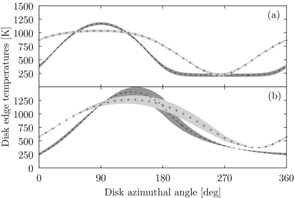
Figure 7. Two different azimuth-dependent temperature models based on the model in Figure 2 are constructed here with Tbasal = 214 K and Tnoon = T(90) = 1, 170 K. Panel a shows a simulated Monte Carlo radiative transfer output where Tbasal = Tmidnight = T(270); and b shows the analytic+MCRT solution as discussed in Section 3.2. The dashed line represents the modeled temperatures across the face of the disk (found every ∼1°), whereas each plus sign shows a predicted, integrated temperature for every 10° of azimuthal angle facing toward the observer. The latter temperatures are integrated over the entire portion of the disk facing the observer, as described in Section 3.2 and represented in Figure 1. Each plus sign represents equivalent SED-determined temperatures one would observe from this unresolved system. Panel b reproduces the observed temperature results at day and night, lending further support of a disk with an off-noon peak and an inherent thermal inertia. The associated error for each modeled temperature distribution is shown by the gray bands.
Download figure:
Standard image High-resolution image3.3. Modeling Error
The implementation of this new method requires an investigation into its effectiveness via its associated error. A number of parameters are considered in this process: the observed temperatures, MCRT density-weighted temperatures Tnoon and Tbasal, and Tmax: night. The nature of this modeling process puts much of the error emphasis on the night calculations.
With the power in the exponential term of Equation (2) assumed to be set, the basal temperature is the only part of the equation that strictly adds uncertainty. However, the point of the cooling equation is to define the disk's azimuthal temperature along the night portion so that an integrated temperature can be obtained to replicate the observations. Therefore, the observed 550 ± 50 K adds its own uncertainty to the model fit, specifically in the adjustment of Tmax: night to provide  . The worst-case error bands shown in Figure 7 result from these uncertainties.
The bands are created by evaluating the model described above with the minimum and maximum temperatures associated with Tbasal and  . Additionally, the error associated with the MCRT noon temperature is used for panel a. Although Figure 7 shows a single model (the same model as presented in Figure 2: a Jupiter-mass disk composed of large, carbon particles at a distance of 740 pc), the error bands are representative of the other modeled systems, because much of the propagated error comes from the observed and MCRT basal temperatures.
Tnoon (1170 ± 25 K) is shown in both panels of Figure 7 at λ = 90°. For panel a, Tbasal = Tmidnight = T(270), whereas Tbasal is used according to Equation (2) in panel b. The dashed lines refer to disk-edge temperatures spaced every ∼1° around its azimuth; the plus sign is the integrated temperature meant to replicate the SED observations. In other words, the plus sign shows the temperature one observes of this unresolved system when a specific λ faces the observer (it is the weighted, integrated temperature of half of the disk facing the observer, as described above). The integrated temperatures at noon, used for comparison to the observations as discussed in Section 4.1, are shown with ±25 K and ±44 K in panels a and b, respectively. The midnight integrated temperatures have similar errors of ±29 K, and ±50 K in each panel. These errors, particularly those from the analytic+MCRT modeling in panel b, are within the same error bands as the observations and allow the analysis to focus on the models with  and
and  .
.
4. RESULTS AND DISCUSSION
4.1. Binned Results
The presented Aurigae models now permit evaluation of the various parameters; to do so, four model bins based on the differences between the observed and modeled day temperatures are defined as follows:
- 1.Likely,;
- 2.Plausible,;
- 3.Unlikely,;
- 4.Highly unlikely,.

There is no bin provided for the three models with  . Therefore, the remaining 33 models are placed in their representative bins: 12 of those 33 models are defined as Likely; 11 are Plausible; and 4 and 6 are defined as Unlikely and Highly unlikely, respectively. Although ∼60% of the total models are Likely and Plausible, ∼40% of the models may not physically represent the system based on their modeled, integrated day and night temperatures, according to the bounds established in this paper. This includes the three models with
  and 10 others with
  greater than 150 K of the observed day temperature. Table 2 gives the Tnoon and Tbasal temperatures of each model but also adds shading according to the defined bins. The bins are segregated into white, light gray, gray, and dark gray, respectively; the three outlier models are shaded in black.
When looking at the various model types that make up the identified bins, we consider the following: distance (740 or 952 pc), disk mass (M⊕ or M♃), dust composition (magnesium–iron silicate, carbon, or a 60/40 mix of those two), and particle size distributions (using MRN cutoffs of 0.001–1 μm, 1–10 μm, or 10–100 μm). The Likely models show a preference for the largest particle size distribution (Nsmall = 2: Nmedium = 3: Nlarge = 7) and carbon (Nsilicate = 3: Ncarbon = 6: Nmix = 3); they also have a slight preference toward a Jupiter-mass disk  and the 740 pc distance (N740 = 7: N952 = 5). The 11 Plausible models preferred the 60/40 mix (2: 3: 6) and the middle particle size distribution (2: 7: 2); they slightly preferred an Earth-mass disk (7: 4) and had no preference toward distance (6: 5). These trends can be identified visually from Table 2.
The main points to consider from the Likely and Plausible models are the tendency toward the larger particle distributions and carbon compositions. The disk mass and distance are not strong dependencies, and when looking at both bins together, the differences wash out between those variables. The distance dependence is somewhat expected, as the physical parameters of the system scale proportionally with distance. However, although an analysis of the disk-edge temperatures did not distinguish between distance, an analysis of the internal disk temperatures may provide a solution. For instance, the 740 pc models provide cold midplane disk temperatures of ∼300 K at ∼4 AU, whereas the 952 pc models have midplane temperatures 2–3 times greater. The large optical depth of the disk revealed by the near-infrared interferometric imaging is also consistent with a cold midplane disk temperature (Kloppenborg et al. 2010). Disentangling these details is an important aspect of future modeling efforts.
As a simple assumption (outlined in Section 2.3 and described in Muthumariappan and Parthasarathy 2012), if the disk is young (denoting q > 1), the composition is expected to be like the ISM. Therefore, a single Likely model has this prescription: a 60/40 mix of large particles in a Jupiter-mass disk. If the disk is older (with q > 1), five Likely models remain and span all compositions, particle sizes, and disk masses. Nevertheless, this simple, physical assumption helps to limit the possible parameters.
For completeness, an analysis of the Unlikely and Highly unlikely bins helps to identify portions of the parameter space that may not physically represent the Aurigae system. The Unlikely bin included only four models and was split evenly between the two masses and distances; the composition was also split between the magnesium–iron silicate and the 60/40 mix, while the particle size followed suit between the small and medium distributions. The six Highly unlikely models all consisted of the smallest particle distribution (6: 0: 0) while slightly preferring the silicates over carbon (4: 2: 0) and a Jupiter-mass disk (2: 4); distance, of course, was evenly spread.
The presented modeling method and subsequent analysis confirms previous assertions of the presence of larger particles within the disk, distinguished by the relatively featureless spectrum of Aurigae (Stencel et al. 2011). This also provides additional support for a carbon-rich disk, but still no clear explanation of why or how that could be the case. This first-order analysis of the disk-edge temperature confirms the technique's usefulness and allows for additional applications, as described below.
4.2. The Tnoon and ΔT Relationship
One of the most significant findings involves the placement of each model on a plot of Tnoon versus ΔT = Tnoon − Tbasal, or the difference between the maximum MCRT model disk temperature (at λ = 90°) and that model's basal temperature. Figure 8 shows the distribution of an error-weighted linear regression fit of the Likely and Plausible models (Tnoon [K] ≈ 0.81ΔT + 410) and its ±σ. When  is plotted with its ±σ of 1100 and 1200 K, a region of confidence is outlined by the intersection of the fitted regression's ±σ with the ±σ of the observed temperature. The model temperatures are plotted according to the appropriate bin. A group of Likely models (solid black circles) sits within the apparent rhombus region of confidence. The Plausible, Unlikely, and Highly unlikely are scattered above and below this region, generally along the linear regression. Therefore, Figure 8 provides a simple test whether a particular model is a solution candidate (if it falls within the confidence region) or if it is not. It becomes a very convenient way to dismiss models, and hence, parts of the parameter space, especially with the number of models required to explore the vast Aurigae parameter space.

Figure 8. Tnoon and ΔT = Tnoon − Tbasal of each Aurigae MCRT model from the present paper are shown here with a best-fit, weighted, linear regression and its ±σ (black lines). The observational day temperature,  , and its associated error, ±50 K, are shown by the gray lines. The ±σ intersection from the linear fit and
  outline a region of confidence for the MCRT models of the Aurigae system. This region serves as a reference for either the need to further investigate a model as a suitable solution for the system (found within the confidence region) or the dismissal of that model's ability to physically explain the system (found outside the region). The Likely models are found within the confidence region. The models are shown with various point-types according to their particular bin as described in Section 4.1. The shading in Table 2 indicates the models that exist within this region.
Download figure:
Standard image High-resolution imageFurthermore, it is significant to note that the y axis of Figure 8 is not the integrated  used for the binning demarcation of individual models, as in the previous section. The points plotted are the density-weighted averages from the MCRT modeling found in Table 2. In other words, the MCRT output—although possibly inaccurately portraying the temperature distribution around the disk—provides a convenient way to investigate the likelihood of a particular model describing the physicality of the Aurigae system by means of Tnoon and Tbasal. The center of the confidence rhombus lies at
  , making Tbasal = 236 K. This gives a general way to identify if a MCRT model is viable or not.
Several models performed with gas-to-dust ratios =10 were found in their appropriate confidence region, according to their model-fitting bin. Investigations of other model varieties have not been applied or tested, but are necessary for further development. Additionally, increasing the number of models and refining the analytic fitting in Section 3.2 to become more physically based will fine-tune the error-weighted linear fit and constrain allowable model descriptions.
If the degeneracy among these disk-edge solutions cannot be broken sufficiently by increasing the number of models or improving the analytic modeling methods, enhancing the numerical modeling methods becomes essential. Incorporating simple, yet effective means in radiative transfer models to demonstrate the dependence of disk temperatures on specific heat and disk rotation would be ideal, especially in extending these concepts to other disk systems with asymmetric heating and observable rotations. SED-fitting has proven effective for Aurigae by Muthumariappan & Parthasarathy (2012), but observational errors and modeling degeneracies make it difficult as well. The presented method—although degenerate limitations also exist—creates another tool for disentangling the parameters in the disk system and should be enhanced with further SED-fitting investigations. Descriptions of the disk interior will also play a role in sorting through the degeneracies (as described in Section 4.1). In the case of Aurigae, the described region of confidence in Figure 8 becomes an effective medium to limit the number of models for further investigation.
4.3. Application to Observation
Both the MCRT and the combined analytic+MCRT models solve for the disk-edge temperatures around the entire disk azimuth. Figure 7 displays these temperatures by the dashed line in both figure panels. Using those predicted temperatures, integrated temperatures are shown every 10° by the plus sign demarcation. Recall that the integrated temperatures are calculated by integrating over the entire portion of the disk facing toward the observer, as was done in Section 3, using the dashed-line temperatures included in each plot. For example, the T(λ⊕ = 90°) point uses the temperatures from ∼0° to ∼180°, giving the integrated temperature of the disk when λ = 90° is pointed toward the observer (hence, the λ⊕ symbol).
Panel a in Figure 7 creates simulated disk azimuthal temperatures based on a slightly altered version of the radiative equilibrium equation equating the dust irradiation temperature with the incoming B5V and F0Ia star radiation presented in Takeuti (2011):

The same stellar parameters as outlined in Table 1 are used for the calculations. In addition, the cos λ term accounts for the angle at which the F0Ia star radiation reaches the disk edge, whereas the η factor acts as a sort of absorptive coefficient. These plots simulate the disk temperature results of a complete 3D MCRT analysis. Panel a is equivalent to a MCRT output of Tnoon = T(90) = 1170 K and Tbasal = Tmidnight = T(270) = 214 K; these values are close to the mean temperatures of all of the Likely and Plausible models.
Panel b of Figure 7 is the result of following the new analytic+MCRT procedure outlined at the beginning of Section 3, using the same prescribed temperatures as in panel a. However, Tbasal is not taken as T(270), but rather the ambient temperature in Equation (2). The most apparent difference between panels a and b is the position and value of the maximum and minimum temperatures.
Figure 7(a) does not reproduce either of the 1150 K or 550 K observed temperatures. The integrated day temperature—with the observer-facing disk azimuth of λ⊕ = 90°—is  , more than 2σ less than
  . The integrated night temperature, at λ⊕ = 270°, is 254 K, almost 6σ lower than
  . This demonstrates the concern of using strictly MCRT SED-fitting, which cannot reproduce either of the observed temperatures.
If the temperatures in Figure 7(a) are artificially adjusted to reproduce the observed temperatures, the noon and midnight temperatures now become T(90) = 1300 K and T(270) = 480 K. None of the 36 MCRT models presented here have these characteristics. However, one model fits within the stated ± error in Table 2: the small, 60/40 mix particles in an Earth-mass disk at a distance of 952 pc. Nevertheless, an investigation of its SED underestimates the observed flux and is therefore discarded as a suitable MCRT model. Note that for these artificially adjusted temperatures, ΔT = 820 K, which places it outside the confidence region in Figure 8. Again, this shows that even a fabricated temperature distribution with the same form as a MCRT output—peak at noon and minimum at midnight—may not be a suitable solution for Aurigae.
Figure 7(b) reproduces the observed day and night temperatures with an off-noon peak and a non-basal midnight temperature. The method used to create this temperature distribution uses the MCRT output temperatures in combination with analytical distributions, following the physical description from Takeuti (2011) and the method described in the present paper. This method allows for elevated temperatures between noon and dusk. In fact, the off-noon peak temperature here is ∼1370 K at λ = 133°. The offset peak raises the observed night temperature so that  , even though
  .
.
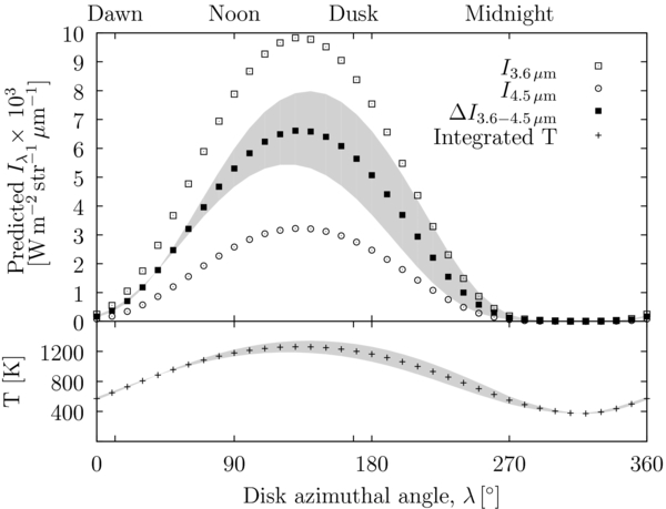
Two observationally distinct properties emerge from an analysis of these two configurations: (1) the offset location of both the peak and minimum integrated temperatures is significant; and (2) the rate of change of the integrated temperatures is different. If the disk can be modeled by the MCRT, it implies a peak at noon and a minimum at midnight, with a dT/dλ ≈ 0 for more than 30° around both of the extrema. If the temperatures are affected by a disk heat capacity (and subsequent thermal inertia), then the peak will be off-noon and the minimum will be close to λ ∼ 0°. Careful observational monitoring will distinguish between the two. In fact, a series of Spitzer Infrared Array Camera (IRAC) observations are underway (and have been since 2009) to monitor the time-dependent, photometric flux variations of the disk in the 3.6 and 4.5 μm bands, in collaboration with Donald Hoard and Steven Howell. Figure 9 shows our predicted specific intensities associated with each of Spitzer's bands (open squares and circles) and the difference between them (filled squares).
Figure 9. This shows predicted specific intensities for λ = 3.6 μm (open squares) and 4.5 μm (open circles) corresponding to the predicted temperatures (bottom panel) of the analytic modeling method presented in Section 3.2 and Figure 7(b). The filled squares show the difference between those two indices and coordinate with ongoing observations from Spitzer's IRAC. The predicted Iλ's at the system is kept in units of W m−2 str−1 μm−1 to refrain from singling out a specific distance. The errors associated with the predicted temperature and corresponding specific intensity differences are shown by the gray bands.
Download figure:
Standard image High-resolution image
The time needed to observe an entire disk rotation period is dependent on the combination of the distance and observed disk rotation speed ∼30 km s−1. Assuming Keplerian rotation, the disk rotation period is around 5 or 7 yr, depending on the size of the disk. These timescales are much less than the evolutionary timescale of a typical disk (∼ 1 Myr), allowing us to be confident that no significant dynamical changes are seen as the disk rotates. Additionally, the rotation period is four to five times less than the system's orbital period. The results of the observations will substantiate the presence, impact, and utility of the heating/cooling effect in the Aurigae disk.
Current work is underway to enhance the described method to accurately model the entirety of the disk's edge temperature. Future iterations of this first-order method will focus on replacing analogous physical descriptions for the assumed shape of the time-dependent temperature distribution, thereby decreasing the overall uncertainty in the methodology and increasing sensitivity of the models. Further iterations will also consider the eccentricity of the system (e ∼ 0.3) and how it plays a role in the temperature distribution within the disk. As the world's telescopes increase their precision and sensitivity, further evidence of asymmetric disk heating will be found in other binary systems projecting some asymmetric configuration, leading to a similar situation as in Aurigae. The ability to produce time-dependent dust temperatures associated with heat capacities and rotations in the given system will be essential in determining the characteristics of the dust and, thereby, the system itself.
5. CONCLUSION
This paper provides the first MCRT modeling of the entire Aurigae system in coordination with analytical calculations that span the parameter space available to the system. The output temperatures of the MCRT modeling are used with first-order approximations of the disk's temperature profile along its azimuthal disk edge. This procedure leads to trends in the models and, with further refinement of the heating and cooling physical applications, will break degeneracies in the solution. Specifically, the models point to carbon-rich particles with a MRN particle size distribution spanning radii of ∼10–100 μm in a Jupiter-mass disk. The analytic+MCRT models do not distinguish between distances of 740 or 952 pc.
The combination of the analytic and MCRT modeling establishes a useful correlation between the MCRT temperatures of Tnoon and Tbasal. The intersection of a weighted linear regression of the model temperatures with the observed day temperatures (and correlated error of ±50 K) creates a region of confidence where the best-fit models conveniently reside. This permits other MCRT models to be compared to this region of confidence as a first-order tool to determine if the model is a plausible solution to consider for Aurigae.
We also make predictions regarding future observations to distinguish if the disk's heat capacity plays an important role in the heating and cooling of the disk. The presence of a time-dependent temperature in the disk refers to material properties of the disk itself, including composition, particle size, and possibly disk mass. Therefore, understanding the disk heating and cooling processes provides a method of determining disk properties in systems without identifiable spectroscopic features.
We would like to acknowledge the continual assistance with the Hyperion code from Dr. Thomas Robitaille and the useful discussions with Brian Kloppenborg and Kathy Geise. We thank the referee for useful comments and suggestions. This work was supported in part by the bequest of William Herschel Womble in support of astronomy at the University of Denver, as well as a Grant-In-Aid of Research from the National Academy of Sciences, administered by Sigma Xi, The Scientific Research Society, for which we are grateful.