


ABSTRACT
In the present series of papers we propose a consistent description of the mass loss process. To study in a comprehensive way the effects of the intrinsic magnetic field of a close-orbit giant exoplanet (a so-called hot Jupiter) on atmospheric material escape and the formation of a planetary inner magnetosphere, we start with a hydrodynamic model of an upper atmosphere expansion in this paper. While considering a simple hydrogen atmosphere model, we focus on the self-consistent inclusion of the effects of radiative heating and ionization of the atmospheric gas with its consequent expansion in the outer space. Primary attention is paid to an investigation of the role of the specific conditions at the inner and outer boundaries of the simulation domain, under which different regimes of material escape (free and restricted flow) are formed. A comparative study is performed of different processes, such as X-ray and ultraviolet (XUV) heating, material ionization and recombination,  cooling, adiabatic and Lyα cooling, and Lyα reabsorption. We confirm the basic consistency of the outcomes of our modeling with the results of other hydrodynamic models of expanding planetary atmospheres. In particular, we determine that, under the typical conditions of an orbital distance of 0.05 AU around a Sun-type star, a hot Jupiter plasma envelope may reach maximum temperatures up to ∼9000 K with a hydrodynamic escape speed of ∼9 km s−1, resulting in mass loss rates of ∼(4–7) · 1010 g s−1. In the range of the considered stellar-planetary parameters and XUV fluxes, that is close to the mass loss in the energy-limited case. The inclusion of planetary intrinsic magnetic fields in the model is a subject of the follow-up paper (Paper II).
Export citation and abstract BibTeX RIS
1. INTRODUCTION
Close-orbit exoplanets in the vicinity of their host stars are thought to be exposed to intense X-ray and ultraviolet (XUV) radiation that deposits a significant amount of energy in the upper layers of the planetary atmosphere. The fact of the presence of Jupiter-type giant planets at orbital distances of ⩽0.1 AU (so-called hot Jupiters) opens questions regarding their upper-atmosphere structure, the interaction with extreme stellar wind plasma flows (Kislyakova et al. 2013, 2014), and the stability against escape of atmospheric gas (e.g., Guillot et al. 1996). Lammer et al. (2003) were the first to show that a hydrogen-rich thermosphere of a hot Jupiter at close orbital distance will be heated to several thousand Kelvin such that hydrostatic conditions will no longer be valid and the thermosphere will dynamically expand. The stellar XUV radiation energy deposition results in heating ionization and the consequent expansion of the planetary atmosphere, which appear to be major driving factors for the mass loss of a planet (Lammer et al. 2003; Yelle 2004; Erkaev et al. 2005; Tian et al. 2005, 2008; García Muñoz 2007; Penz et al. 2008; Guo 2011, 2013; Koskinen et al. 2010, 2013; Lammer et al. 2013). Applied hydrodynamic (HD) models by Yelle (2004), Tian et al. (2005), García Muñoz (2007), Penz et al. (2008), Lammer et al. (2009), and Guo (2011), (2013) and empirical models by Koskinen et al. (2010) also indicate that close-in exoplanets experience extreme heating by stellar XUV radiation, which results in atmospheric expansion and outflow up to their Roche lobes (e.g., Erkaev et al. 2007) with mass loss rates of ∼1010–1011 g s−1. These loss rates are also supported by Hubble Space Telescope (HST)/Space Telescope Imaging Spectrograph (STIS) observations (Vidal-Madjar et al. 2003, 2004), which detected a 15% ± 4% intensity drop in the high-velocity part of the stellar Lyα line during the planet (HD 209458b) transit, which was interpreted as a signature of neutral H atoms in the expanding planetary atmosphere.
The problem of upper atmospheric erosion of close-orbit exoplanets and their mass loss is closely connected with the study of the whole complex of stellar–planetary interactions, including consideration of the influences of intensive stellar radiation and plasma flows (e.g., stellar winds and coronal mass ejections) on the planetary plasma and atmosphere environments. The following effects have to be considered in that respect.
- 1.The XUV radiation of a host star affects the energy budget of the planetary thermosphere, resulting in the heating and expansion of the upper atmosphere, which under certain conditions could be so large that the majority of light atmospheric constituents overcome the gravitational binding and escape from the planet in the form of a hydrodynamic wind (Yelle 2004; Tian et al. 2005, 2008; Penz et al. 2008; Koskinen et al. 2010, 2013; Erkaev et al. 2013; Lammer et al. 2013). This contributes to the so-called thermal mass loss process of atmospheric material.
- 2.Simultaneously with the direct radiative heating of the upper atmosphere, the processes of ionization and recombination as well as production of energetic neutral atoms by sputtering and various photochemical and charge exchange reactions take place (Yelle 2004; Lammer et al. 2008; Shematovich 2012; Guo 2011, 2013). Such processes result in the formation of extended (in some cases) coronas around planets, filled with hot neutral atoms.
- 3.The expanding, XUV-heated and photochemically energized, upper planetary atmospheres and hot neutral coronae may reach and even exceed the boundaries of the planetary magnetospheres. In this case they will be directly exposed to the plasma flows of the stellar wind and coronal mass ejections with the consequent loss due to an ion pickup mechanism. That contributes to the nonthermal mass loss process of the atmosphere (Lichtenegger et al. 2009; Khodachenko et al. 2007b). A crucial parameter here appears to be the size of the planetary magnetosphere, characterized by the magnetopause standoff distance RS (Khodachenko et al. 2007a, 2007b; Lammer et al. 2009; Kislyakova et al. 2013, 2014). Altogether, this makes the planetary magnetic field and the structure of the magnetosphere, as well as the parameters of the stellar wind (e.g., density nsw and speed vsw), very important for the processes of atmospheric erosion and mass loss of a planet.
The background magnetic field of a planetary magnetosphere not only forms a barrier for the upcoming plasma flow of a stellar wind, but it also influences the outflow of the escaping planetary plasma wind formed in the course of atmosphere heating and ionization by stellar XUV. For example, Adams (2011) considered outflows from close-in gas giants in the regime where the flow is most likely controlled by magnetic fields. In that respect it is important to note that the processes of material escape and planetary magnetosphere formation have to be considered jointly in a self-consistent way in their mutual relation and influence. The expanding partially ionized plasma of a hot Jupiter atmosphere interacts with the planetary intrinsic magnetic field and appears to be a strong driver in the formation and shaping of the planetary magnetosphere (Adams 2011; Trammell et al. 2011; Khodachenko et al. 2012), which in its turn influences the overall mass loss of a planet.
The different modeling approaches proposed so far for the simulation of planetary atmosphere expansion (Yelle 2004; Erkaev et al. 2005; Tian et al. 2005, 2008; Penz et al. 2008; Guo 2011; Koskinen et al. 2013; Lammer et al. 2013), in spite of the inclusion sometimes of a lot of details regarding the atmospheric composition and photochemistry processes, quite often miss important basic processes or operate with strong idealizations and simplifications (e.g., a non-self-consistent prescription of the XUV-heated region or neglect of gas ionization–recombination processes). Moreover, the effects of a background planetary magnetic field are usually not considered at all or again are included in a non-self-consistent way (e.g., by prescribing specific magnetic configurations; Trammell et al. 2011).
The investigation of exoplanetary magnetospheres by means of numerical simulations requires an efficient and well-organized model capable of supporting a comparative study of different physical effects and processes that contribute to the formation and shaping of the magnetosphere. To investigate all of the relevant processes and the role of the planetary intrinsic magnetic field in the process of atmospheric material escape and mass loss, as well as the formation and structuring of the planetary inner magnetosphere in a self-consistent way, we adopt a two-step modeling strategy, starting (as a first step) with a hydrodynamic (HD) model of atmosphere expansion, which is presented in this paper. After having developed a comprehensive model for an expanding upper atmosphere of a hot Jupiter, we will perform, as a next step, the MHD modeling, with the inclusion of planetary intrinsic magnetic fields and a study of their role in the formation of the inner magnetosphere and atmosphere mass loss. This part of our investigation will be reported in the follow-up paper.
Therefore, the major purpose of this paper is to develop a general and simple (comprehensive) enough model of an expanding atmosphere of a hot Jupiter that includes all of the major effects and yields results that are consistent with the studies and findings reported by other research groups (Yelle 2004; Erkaev et al. 2005; Tian et al. 2005; Penz et al. 2008; Guo 2011; Koskinen et al. 2013; Lammer et al. 2013). Stellar XUV radiation absorbed in a self-consistently defined inner layer of the modeled atmosphere is a major energy deposition source and driver for the atmosphere expansion. The effects of radiation absorption and reemission as well as atmospheric gas ionization and recombination and the gravity of a planet are included in the model. Special attention in the present numerical modeling is paid to the analysis and deeper understanding of the major drivers and physical effects that result in the expansion of atmospheres of close-orbit exoplanets. While considering a simple hydrogen atmosphere model, we include the effects of radiative heating and ionization of the atmospheric gas and adiabatic and radiative cooling, and we impose more general (compared to previous studies) boundary conditions and study their influence on the simulation results. In addition, the influence of the additional inclusion of  cooling on the model behavior is tested.
Special attention in the present study is paid to an investigation of the different regimes of a hot Jupiter atmosphere expansion that are related to two basic types of one-dimensional (1D) HD solutions, characterized by the presence of a well-formed expanding plasma wind (free-outflow regime) or by just an insignificant slow material escape (restricted-flow regime). In our model such a distinction is achieved in a natural way by choosing different types of outer boundary conditions. As typical parameters for the modeled hot Jupiter planet we take those of HD 209458b (i.e., Rp = 1.4RJ, Mp = 0.7MJ) orbiting a Sun-like star at a distance of 0.05 AU.
For a more clear separation of the various active factors influencing the formation of an exoplanetary magnetosphere, our numerical study is aimed at a simulation of only the expansion of the plasma without the inclusion of rotation effects. This can be justified for the case of tidally locked close-orbit hot Jupiters where the rotational angular velocity of the planet is equal to that of the orbital revolution and is relatively small. In this case, the radial expansion of the hot planetary plasma will dominate the corotation effects in the inner magnetosphere.
The paper is organized in the following way. In Section 2 we address the issue of XUV heating and radiation transfer in the upper atmosphere, which plays a crucial role in the modeling of a hot Jupiter mass loss. In Section 3 the modeling concept is presented, including the atmosphere expansion drivers and the role of the different types of boundary conditions in that respect. Section 4 is devoted to the major equation of the presented model and key assumptions. Section 5 presents the results of the numerical modeling and related basic regimes of atmosphere expansion of a hot Jupiter connected with the specific boundary conditions applied. A possible influence of an intrinsic planetary magnetic field on the expansion flow is addressed and investigated in a number of specific cases. A comparative study of the role of different physical effects included in the model, such as XUV heating, material ionization and recombination, infrared cooling, adiabatic and Lyα cooling, and Lyα reabsorption is also presented in Section 5. In Section 6 we discuss the obtained results and their relevance for hot Jupiters.
2. XUV HEATING AND RADIATION DIFFUSION IN THE UPPER ATMOSPHERE
A crucial issue concerns the details of the XUV heating process. The deeper the heated layer of the thermosphere, the higher the energy needed for photons to be able to reach it because the XUV absorption cross section decreases with the increasing energy of a photon as σXUV ∼ 1/(hν)3. An energetic photoelectron created during photoionization of a hydrogen atom by a photon with energy ε = hν carries the excess energy hν − Eion, where Eion is the ionization energy. This excess energy may be lost by the photoelectron in different ways (briefly addressed below) before it will reach a thermal balance with the entire hydrogen atoms, ions, and background electrons.
For the typical conditions realized in the modeled upper thermosphere, the fastest route for energy loss by a photoelectron is Coulomb collisions with background ions and electrons. The efficiency of heating by this process is ηh ≈ 100%. However, deeper in the atmosphere (i.e., closer to the planet surface), the degree of ionization and plasma density falls, whereas the density of neutrals sharply increases. At these conditions, when the density of neutrals is higher than ∼1010 cm−3, the photoelectron cools down more efficiently through inelastic collisions with atoms (and its energy exceeds the excitation or ionization potential of a hydrogen atom).
Only after having lost its energy down to values below E21 ≈ 10 eV (the excitation energy), the photoelectron will start sharing the rest of its energy with the background medium through elastic collisions with hydrogen atoms. Therefore, each absorbed XUV photon in the dense thermosphere transfers into direct thermal heating of the gas a value not exceeding on average 10 eV. The excess energy is spent mostly on Lyα emission and cascading ionization. In the course of the cascading ionization, the photoelectron shares with a newly released electron, on average, an energy of about (0.2 − 0.5)Eion (Kim et al. 2010). Thus, only about 0.17–0.33 of the energy hν − Eion ≫ Eion goes into heating of the overall gas in this way. At high energies (≫Eion), the cross section of excitation of hydrogen by electron impact and subsequent reemission of Lyα photon is about the same as that of ionization (see, for example, Shah et al. 1987; Sweeney et al. 2001). For this energy-loss channel everything depends on how optically thick the given layer of thermosphere for Lyα photons is. In the case of sufficiently high optical thickness, all of the energy of the photoelectrons eventually returns to the background electrons due to impact deexcitation. In the opposite case it is all lost, and the heating efficiency reduces. Therefore, the heating efficiency ηh of XUV may vary from about 58–67% deep in the thermosphere, down to lower values (up to ∼8–17%) in the dense layers, which are optically thin for Lyα, to 100% in a fully ionized outer plasma envelope. Accordingly, a wide range of applied heating efficiencies ηh ∼ 15–60% can be found in the related studies (Chassefière 1996; Yelle 2004; Lammer et al. 2009; Koskinen et al. 2013; Erkaev et al. 2013; Lammer et al. 2014). A saturation value of 93% was used in Koskinen et al. (2013). The average value most often used for the efficiency of XUV heating in the studies of exoplanet giants is ηh = 50%. That is the value we apply in our modeling. For an accurate calculation of the energy transport process, a kinetic model of photoelectron diffusion is needed (Cecchi-Pestellini et al 2009). In that respect we note that there is an obvious distinction between the net efficiency of absorption ηnet, which equally affects ionization and heating rates, and the heating efficiency ηh, which concerns only heating.
At this point the reabsorption of Lyα emission should also be addressed. For typical temperatures of ∼104 K the cross section of Lyα photon absorption σLα by atomic hydrogen near the line center is in the range of 10−15 to 10−14 cm2. This is much larger than the XUV absorption cross section. Therefore, the thermosphere regions with the most intense XUV heating will be optically thick for Lyα, and the cooling efficiency of the latter will be diminished. It is important to evaluate how strong this effect may be because it results in higher temperatures and higher densities in the "dead zone" of a hot Jupiter magnetosphere and also influences the separation between "wind" and "dead" zones. For that purpose in Section 4.2 we adopt a simple model of Lyα photon spatial diffusion with a coefficient of ∼c/naσLα as determined by the distance and time intervals between the consequent reabsorption events, but we ignore the spectral diffusion of photons from the line center.
3. MODELING CONCEPT
As specified in the overall description of our two-step modeling strategy presented in the introduction, the major goal of the present work is to understand the hydrodynamic behavior of a hot Jupiter's expanding upper atmosphere without including the effects of the background magnetic field of the planet. This goal may be achieved with a 1D HD model that takes into account the most important physical processes, which we discuss below. Even a simplified 1D HD model that deals with a one-gaseous-component (hydrogen) atmosphere and contains only the most important elements and physical processes such as heating by stellar XUV radiation, atmospheric gas ionization and recombination, as well as radiative and adiabatic cooling of the expanding planetary plasma wind, is not yet fully developed and understood because of the complex physics involved. In the present paper we propose our version of such a model.
A widely used simplification, we also disregard the fact that a star illuminates only one side of a planet and assume an azimuthally symmetric radiation flux, taking into account the reduced value of ηnet equal to 0.5. This approach is commonly accepted as a good approximation that enables one to avoid two-dimensional (2D), or extremely complex three-dimensional (3D), modeling without loss of essential physics.
3.1. Atmosphere Expansion Drivers
In the first studies of the planetary atmosphere expansion aimed at estimating the material escape rate and related mass loss, an isothermal Parker-type solution was imposed with an a priori prescribed boundary condition at the planetary inner atmosphere (or surface) related to the XUV heating of a fixed, predefined thin layer (Watson et al. 1981). However, it was shown in Tian et al. (2005) that in a thin-layer-heating approximation the expanding atmosphere mass loss rate strongly depends on the altitude of the layer where the radiation energy is deposited.
Moreover, as was suggested already by Parker, the realistic solution that corresponds to an outflowing (expanding) wind regime requires an additional volume heating in order to compensate for the adiabatic cooling of the expanding gaseous envelope. This was also confirmed in the follow-up numerical modeling studies. For example, in the case of the solar wind, an additional acceleration factor is called for to appear at a few solar radii. This additional driver is attributed to the dissipation of Alfvén waves (Usmanov et al. 2011). For an outflowing atmosphere of a hot Jupiter, one of the possible candidates for the role of such a distributed accelerator is the absorption of XUV, which takes place everywhere where atomic or molecular hydrogen is present. However, it turns out that at distances of about several planetary radii, where the additional forcing of the expanding planetary atmospheric material is needed to keep it in the outflowing regime (i.e., to escape the gravity tension), the gas is highly ionized, and the absorption of XUV decreases.
Nevertheless, the same fact of the increasing ionization degree, which reduces the efficiency of XUV heating, contributes to the additional acceleration of the wind and appears as an additional booster of the planetary plasma wind. That is because the thermal pressure p = (na + ni + ne)kT increases (up to two times) at certain intervals of heights (in the ionization region) because of the contribution of the electron and ion pressure, whereas the density of material ≈(na + ni)mi remains practically unchanged. The created pressure gradient provides an additional driving force for the expansion of ionized atmospheric material. Here we use the standard notations with na, ni, ne, mi, k, and T standing for the number density of neutrals, ions, electrons, ion mass, Boltzmann constant, and temperature, respectively. In the course of the ionization, the expanding atmospheric wind experiences in the ionization region an additional acceleration and reaches velocities that sustain the continuous outflow regime. Note that the adiabatic cooling and the plasma pressure gradient mechanism caused by the ionization act opposite to one another, and the simple isothermal model that does not consider them properly produces an erroneously too strong planetary wind. To our knowledge, the role of the ionization layer and acceleration of the atmospheric plasma by the pressure gradient were not elucidated thus far for the problem of a hot Jupiter plasma wind generation. At the same time, this effect is implicitly included in several reported simulations (e.g., García Muñoz 2007; Guo 2011, 2013; Koskinen et al. 2010, 2013).
3.2. Inner Boundary Conditions
Properly defined boundary conditions at the inner edge of the simulation box appear to be a crucial issue for the models of atmosphere expansion driven by XUV heating. These boundary conditions are usually associated with a deep layer of inner planetary atmosphere, which we conventionally call a planet surface.
Besides the plasma outflow and the related adiabatic cooling, because of plasma expansion, another efficient energy drain that acts to compensate for the XUV heating is an excitation of the second level of hydrogen atoms by electron impact and fast emission of Lyα photons (Murray-Clay et al. 2009). At the same time, because of the exponential decrease with temperature, this mechanism can fully compensate for XUV heating of the deep and cold layers of the thermosphere if the latter decreases with height fast enough. However, because of the wide spectrum of stellar XUV illuminating a planet, its heating rate decreases with height (i.e., with the increase of integrated column density), not exponentially, but more likely as a power law. Therefore, a model that is based only on the Lyα cooling requires a limiting inner boundary at the layer with a temperature of several thousand Kelvin. To admit this condition, one needs an additional justification (i.e., model) for the inner boundary at the lower thermosphere. An estimation of the overall energy budget shows that the inner "cold" thermosphere has to have a temperature of about 1000–2000 K. The cooling mechanism due to infrared emission that involves the H2 and  species is usually addressed in that respect (Yelle 2004). Although complex models that include the major photochemistry effects already exist (Yelle 2004; García Muñoz 2007; Koskinen et al 2007), in the present paper we adopt a bit different and more simple approach to take into account the infrared cooling effects.
While infrared cooling due to  may dominate in the deep thermosphere at pressures larger than ∼1 μbar, it has been concluded in Koskinen et al. (2013), based on a comparison of kinetic and hydrodynamic models, that this process does not affect formation of the expanding planetary wind. In that respect, Koskinen et al. (2013) used a hydrodynamic model with an inner boundary fixed at the level of 1 μbar pressure. On the other hand, regardless of Lyα or infrared cooling, the expanding plasma motion alone, because of the adiabatic cooling mechanism, can effectively remove heat from the deep layers of a thermosphere affected by XUV radiation. In some models this effect is known to be so strong that it eventually overcomes the heating and leads to an unrealistic drop in temperature (Watson et al. 1981). However, in a case when radiation (integral over spectrum) attenuates not exponentially but more likely as the inverse power of the density column, the domination by the adiabatic cooling effect is diminished. Below, using the results of an analytical solution that takes into account only adiabatic cooling and a proxy model of XUV heating at large integrated column densities, as well as by means of the numerical simulation, we show that the inner boundary can be extended down to the deeper layers with a much higher pressure on the order of
  . García Muñoz (2007) also arrives at a similar conclusion.
The question of the inner boundary pressure appears to be a crucial one also because, according to Tian et al. (2005) and Trammell et al. (2011), the material escape at low pressures is practically proportional to it. This has to be avoided in a self-consistent model. Therefore, taking the inner boundary sufficiently deep in the atmosphere, where the XUV energy deposition per particle becomes practically zero, seems to be a reasonable choice for a more realistic model that is independent of the particular parameter values at the inner boundary, or in other words, independent of the size of the simulation box. Indeed, we found (Section 5.2) that at pressures starting from  and higher, the obtained solution shows quite weak dependence on
  .
.
Another important modeling parameter related to the inner boundary pressure that has to be properly defined is the base (or the inner boundary) temperature  . General energy budget considerations constrain it to be at around 1000 K. The particular values of 750 K (Yelle 2004), 1200 K (García Muñoz 2007), and 1350 K (Koskinen et al. 2013) were used in the models of a hot Jupiter. In the model presented in this paper the behavior of a hot Jupiter environment insignificantly depends on a particular value of
  . That is due to taking the inner boundary of the simulation box at sufficiently deep layers with high enough pressure that are unaffected by the stellar XUV. At such a deeply located inner boundary, an extremely steep (exponential) density growth takes place such that the condition of a constant mass flux supposes very small values for the velocity. Therefore, taking the velocity to equal zero at the inner boundary does not affect the numerical solution at all if the boundary is sufficiently deep.
Inclusion in the model of deep thermosphere layers with pressures higher than ∼1 μbar requires a certain attention to the infrared cooling effect due to  and an understanding of how it affects the simulation results. To check this, we performed calculations with a proxy model for the infrared cooling with volume rates of about 10−7 erg cm3 s−1 as reported in Yelle (2004) and García Muñoz (2007). The obtained results enable us to conclude that the temperature profile in the inner atmosphere regions (i.e., close to the planet surface) and the corresponding density distribution are somewhat sensitive to the additional energy-loss mechanism related to the infrared cooling (besides the adiabatic and Lyα cooling). However, because of its local character and the action first of all in the deep layers of the inner thermosphere, the
  cooling leads to the reduction of the simulated material escape rate approximately only by a factor of two. Such an insignificant difference gives a reason for an essential simplification of the model of atmosphere expansion and mass loss by ignoring the complex hydrogen chemistry at the base of the cold thermosphere or the use of its simplified modeling approximations.
3.3. Outer Boundary Conditions
An appropriate definition of conditions at the outer boundary also plays an important role in the modeling. Similar to the case of the inner boundary conditions discussed above, it would be reasonable to have the outer boundary conditions also defined such that the obtained numerical solutions are quantitatively independent of them in a sufficiently wide range of parameters.
Besides, it is necessary to distinguish between the two different types of outer boundary conditions that are related to different external physical circumstances. One is an open (or free) outer boundary, when the expanding atmosphere material can leave the vicinity of a planet, i.e., when the escape of mass and energy takes place and the escaping plasma can flow through the outer boundary unaffected. Another situation corresponds to the closed (or shut-up) conditions when the material flow is suppressed or restricted at a certain distance from a planet by some external physical factors not included self-consistently in the model. As an example of such restricting factors, an encountering stellar wind or planetary magnetic field can be referred. The choice of a particular type of outer boundary condition finally depends on the goal of the specific modeling and the region of application of the modeling results. In particular, in the case of a hot Jupiter, modeling of different parts of the magnetized planetary extended thermosphere may require different sets of external boundary conditions.
For example, simulation of a so-called wind zone of a hot Jupiter magnetosphere (Adams 2011; Trammell et al. 2011; Khodachenko et al. 2012) at sufficiently high latitudes where plasma leaves the planet along the open magnetic field lines needs the open outer boundary conditions, whereas modeling of the "dead zone" occupied by a stagnated plasma of an inner magnetosphere locked in the region of closed magnetic field lines would require the closed boundary.
The interaction of the magnetized hot Jupiter with a stellar wind results in the formation of a magnetosphere obstacle located at several planetary radii from a planet. Depending on the character of the encountering stellar wind plasma flow (subsonic or supersonic/Alfvénic), this magnetosphere obstacle can have the form of a paraboloidal shock or Alfvén wing system (Ip et al. 2004; Erkaev et al. 2005; Khodachenko et al. 2012) elongated in the direction of the plasma flow, which for the close-orbit planets also has to take into account the Keplerian velocity of orbital motion of the planet (Grießmeier et al. 2007; Cohen et al. 2011; Khodachenko et al. 2012). Because of these factors, the outer boundary conditions in the first numerical modeling of a hydrodynamic atmosphere escape on a hot Jupiter (Yelle 2004) were imposed at a relatively close distance of only 3 Rp from the planet. Note that a question regarding the interaction of an upcoming stellar wind with the expanding planetary plasma wind and the role of a planetary magnetic field in this process was not considered in Yelle (2004) or in the later modeling cases (García Muñoz 2007; Penz et al. 2008; Guo 2011, 2013; Adams 2011; Trammell et al. 2011; Koskinen et al. 2013; Khodachenko et al. 2012; Lammer et al. 2013; Erkaev et al. 2013). Thus it still remains a subject for future investigation.
4. MODEL EQUATIONS
4.1. Basic Equations and Major Assumptions
In this section we describe the basic equations of the presented numerical model. For simplicity's sake we restrict the modeling by assuming a purely hydrogen atmosphere of a hot Jupiter composed in the general case of hydrogen atoms, ions, and electrons. As has been shown in García Muñoz (2007), Trammell et al. (2011), Koskinen et al. (2010), and Guo (2011), the atomic and Coulomb collisions in the modeled regions of a hot Jupiter upper atmosphere are efficient enough to ensure the "nonslippage" approximation for neutral hydrogen atoms, ions, and electrons such that the assumptions of Va = Vi = Ve = V as well as temperature equilibrium Ta = Ti = Te = T hold true. Here Vk and Tk with k = a, i, e correspond to the velocity and temperature of components of the partially ionized atmospheric gas, respectively, whereas V and T stand for its velocity and temperature as a whole.
For the typical temperatures ⩽104 K realized in the upper atmosphere of a hot Jupiter (Koskinen et al. 2010), the proton–proton Coulomb collision cross section is well above 10−13 cm−2. The proton–hydrogen collisions are dominated by resonant charge exchange with the cross section at the typical velocity of 10 km/ c−1, at approximately 10−14 cm−2. The location of the exobase for a hot Jupiter that corresponds to the region where the Knudsen number  reaches 1 is determined by the condition when the mean free path
  is equal to a typical scale of flow Δ. In the regions far from the planet, Δ may be taken to be on the order of the planetary radius, i.e., Δ ∼ Rp, and the condition Kn ∼ 1 is realized approximately in the layers with density ∼104 cm−3. That remains well above the height range (10 Rp) considered in the modeling simulations. Close to the planet surface, the barometric height H, which is smaller than Rp, has to be taken as the typical scale Δ. However, because of much larger densities there, the mean free path
  also becomes smaller, and the condition Kn < 1 holds true. Therefore, the fluid approach adopted in the present study is fairly valid.
Within the frame of these assumptions, taking into account the processes of hydrogen ionization (by XUV and electron collision) and recombination, the continuity, momentum, and energy balance equations of the model can be written as follows.


where the following notations are used:

In Equations (1)–(4) we use the standard cross sections of major processes, such as ionization by XUV: σXUV = 6.3 · 10−18 cm2; ionization by electron impact:  ; recombination with an electron: σrec = 6.7 · 10−21 T−3/2 cm2; hydrogen excitation and deexcitation:
  and σ21 = 7 · 10−16 T−1 cm2, respectively; Lyα absorption: σLα ∼ (10−15 ⋅⋅⋅ 10−14) T−1/2 cm2 with the temperatures scaled in units of characteristic temperature of the problem (
 ), except for the exponent power indices in the expressions for σion and σ12, where temperature is taken in energy units. In addition, for the wavelength-averaged terms corresponding to XUV ionization and heating rates in Equations (2) and (4) we use the proxy model proposed in Trammell et al. (2011):


where  is the neutral hydrogen column density.
The typical values for the mean ionization time tXUV ≈ 6 hr and mean photoelectron energy (or energy per absorption event) εXUV ≈ 2.7 eV, which goes to heating, are taken in Equations (6) and (7) to correspond to the integrated stellar XUV energy flux of FXUV ≈ 2 × 10³ erg cm−2 s−1 expected at 0.05 AU orbit around a Sun-analog star. Note that the decrease of heating (Equation (7)) is close to an inverse rather than an exponent power of the density column. The reasons to use the proxy model instead of one calculated with the frequency-binned real Solar spectra are as follows. The deviation of the proxy model from the spectrum-based one is sufficiently small to ensure that the error in the computed mass loss rate is less than 25%. Besides that, using the analytical model enables one to make simple analytical estimations of the expected solutions, which help to verify the correctness of the obtained numerical results (Section 5.2) and to understand the physics of the involved processes.
To take into account the fact that the star illuminates only one side of the planet, in our calculations we reduce the radiation flux (and the corresponding values given by Equations (6) and (7)) by a factor of two, i.e., take ηnet = 50%. In addition, to be definitive we suppose the heating efficiency ηh of stellar XUV (Chassefière 1996; Yelle 2004; Lammer et al. 2009; Koskinen et al. 2013) to be 50% and therefore divide by two once more the outcome of Equation (7), which is then used as an approximation for the term 〈(EXUV − Eion)σXUVFXUV〉 in the energy Equation (4).
4.2. Energy Balance and Radiation Diffusion Equations
Besides the XUV heating term and adiabatic cooling due to plasma expansion (the last term at the left-hand side of Equation (4)), the energy Equation (4) also takes into account energy loss and gain due to excitation and deexcitation of the n = 2 level of hydrogen atom by electron impact as well as cooling due to ionization. We assume that the concentration of excited atoms remains sufficiently low, i.e., na, n = 2 ≪ na, n = 1 ≈ na. The validity of this assumption is specially verified in the course of the modeling simulation. Because of a too-low rate at the considered densities, we also neglect in Equation (2) the process of three-body recombination, which is the reverse of the inelastic impact ionization.
To complete the energy Equation (4) one has to define a way to calculate the concentration na, n = 2 of the excited atoms at the level n = 2. In our model it is controlled by the density of the Lyα photons that are emitted by the excited atoms and reabsorbed by the atoms in a nonexcited state (i.e., level n = 1). In the case of an optically thin gas envelope, the concentration of excited atoms remains very small (negligible) because of fast radiative deexcitation. On the other hand, in the optically thick case, the concentration na, n = 2 may remain moderately high because of Lyα photon sequential reabsorptions until the photons leave the system. Such a process of multiple reabsorptions and reemissions of a photon with a chaotic change of its travel direction (after each reemission act) can be described in the first approximation as diffusion with a coefficient determined by the average distance (naσLα)−1 and velocity c between reabsorptions. The corresponding diffusion equation for the Lyα photons density NLa and concentration of excited atoms may be written as follows.

The terms in the right-hand side of Equation (9) stand for the photon emission by the excited atoms with mean emission time τ21, absorption by nonexcited atoms, and spatial diffusion, respectively. For the typical scale of a system, which approximately equals Rp ∼ 1010 cm and σLa ∼ 10−15 cm2, the gas becomes optically thick for Lyα photons at densities above 105 cm−3.
Introducing a normalized number density of Lyα photons  , the stationary concentration of the excited atoms may be expressed from Equation (8) as
By substitution of this solution in Equations (4) and (9) and taking into account that na, n = 1 ≈ na, we obtain a modified energy-balance equation and the equation for normalized number density of Lyα photons:
Because the emission time τ21 ∼ 1 ns is very small, we neglect the terms proportional to Λe · σ12τ21 and Λe · σ21τ21 in the final form of the Equations (11) and (12), as compared with one.
When the system is essentially optically thick, the diffusion term in Equation (12) tends to zero, and the number density of Lyα photons saturates at a level where collisional excitation and deexcitation balance each other, resulting in  . Note that for temperatures T ≪ E21 the population of excited atoms is much smaller than that of nonexcited, ground-state atoms:
  . In that respect, one of the reasons for inclusion in Equation (11) of a relatively unimportant electron impact ionization term is to ensure a nonzero cooling in the case of total saturation of the n = 2 level by Lyα photons.
Further on, we represent the temperature and velocity of the simulated upper atmospheric material in units that correspond to the characteristic temperature of the problem taken as  and the corresponding
  , whereas the distances will be normalized to a typical scale of the system, defined by planetary radius Rp.
5. SIMULATION RESULTS
The numerical solution of the model Equations (1)–(3), (11), and (12) was performed with an explicit second-order differential scheme on a nonuniform grid with a mesh size taken to be proportional to the radial distance to resolve the decreasing barometric scale height near the planet surface. The dimensionless mesh size (normalized to Rp) at the inner boundary was taken (depending on the particular run) as Δrmin = (1 − 2.5) · 10−3. The time step was constant and on the order of Δt ⩽ 10−1Δrmin . Discretization is centrally based. Time marching is a simple one-stage explicit iteration. A stationary solution is sought with convergence criteria defined as the relative change of calculated values (for example, of the mass loss) at the outer boundary at one step not exceeding 10−4. Usually it takes several hundred to several thousand dimensionless times or 105–106 iterations to achieve the steady state. A spherical geometry with all physical values varying only along the radial distance was considered. Because of the large density gradients realized in the course of the simulation, to increase the accuracy of calculations, instead of real density values in the continuity Equation (1) we dealt with ln (n). In order to suppress the instability of the numerical scheme related to generation of acoustic-gravity waves, a small artificial viscosity term ∇η∇V was added in the momentum Equation (3) with a numerical coefficient η of about 10−5 in dimensionless units.
The initial profile of the neutral thermosphere density in hydrostatic and isothermal equilibrium is given by the solution of Equation (3) in the steady state:
where  is an important dimensionless parameter of the system, defined as the relation of thermal energy to gravitation escape energy at the inner boundary of the simulation region, r = 1 (in units of Rp), i.e., close to the conventional planet surface. For the considered parameters of a hot Jupiter, λ has a typical value of about 10. The coefficient before the exponent in Equation (13) is taken such that the density value at the inner boundary of the simulation region corresponds, for the given temperature, to the pressure of
  . At the same time, from the computing point of view, the exact position of this boundary (at the surface of a planet, or slightly above—in the deep atmosphere) is not important because of a very steep dependence of density on r at the initial dimensionless temperature To = 0.1, which corresponds to an absolute inner boundary temperature value of
  .
.
5.1. Two Basic Regimes of Atmosphere Expansion
Below we consider numerical solutions of a spherical 1D HD model that describe different behavior regimes of a hot Jupiter's upper atmosphere, corresponding to the two basic types (open and closed) of outer boundary conditions.
The position of the outer boundary is taken such that the results of the calculations, such as the mass loss rate, do not depend on the distance of its particular location. The question discussed in the literature is the position of the exobase relative to the model outer boundary. For HD modeling of some particular hot Jupiters (e.g., HD 209458b), it was shown in several papers that the exobase is farther than 10 Rp. Thus in our modeling we also take the location of the outer boundary at 10 Rp, where the numerical solution practically does not depend on the boundary's exact position and the use of hydrodynamic modeling approach is justified. More detailed (García Muñoz 2007) or partially kinetic conditions (Koskinen et al. 2013) also lead to similar results and conclusions.
When the cooling mechanism due to Lyα radiation is taken into consideration, the model admits two general solutions related to the global energy balance. One of the solutions represents the case already mentioned above with an atmospheric material free outflow when the XUV heating is balanced by the advection and adiabatic cooling. Another solution corresponds to a restricted-flow regime, in which the XUV heating is balanced mostly by Lyα cooling. The particular values of physical quantities are also different for these two types of solutions. The restricted-flow solution is characterized by a hotter and about an order of magnitude denser stagnated plasma envelope. An important issue regarding the free-outflow and restricted-flow solutions is that their realization in our model is completely controlled only by the specific outer boundary conditions. Note that the free-outflow and restricted-flow regimes are physically relevant (and may be attributed) to the "wind" and "dead" zones of a hot Jupiter magnetosphere, respectively (Trammell et al. 2011; Khodachenko et al. 2012).
As mentioned above (Section 3.2), the Lyα cooling is inefficient at temperatures below several thousand Kelvin. Therefore, a small outflow of material is needed to compensate for the excess XUV heating in such a dense deep thermosphere. In that respect, instead of a totally closed (shut-up) condition at the outer boundary, we allow a small flow of material at a speed on the order of 0.1 km s−1. This in fact constitutes the matter of the restricted-flow regime. Such an assumption is relevant for the conditions in a "dead zone" of a hot Jupiter's inner magnetosphere or in the front region of interaction with a stellar wind because a small portion of the planetary plasma might still leave the planet there by convection to higher latitudes or to the tail.
To deal with the open outer boundary in practice, we assume the spatial derivatives of physical values to be small, i.e., asymptotically approaching zero with a decreasing mesh size and increasing distance.
A similar approach to the study of atmosphere expansion regimes was adopted for the first time in García Muñoz (2007), where instead of velocity a fixed pressure was imposed at the outer boundary, and solutions with an escaping material flow varying from a supersonic up to a slow subsonic one were obtained.
5.2. Free-outflow Regime of a Hot Jupiter's Atmosphere Expansion
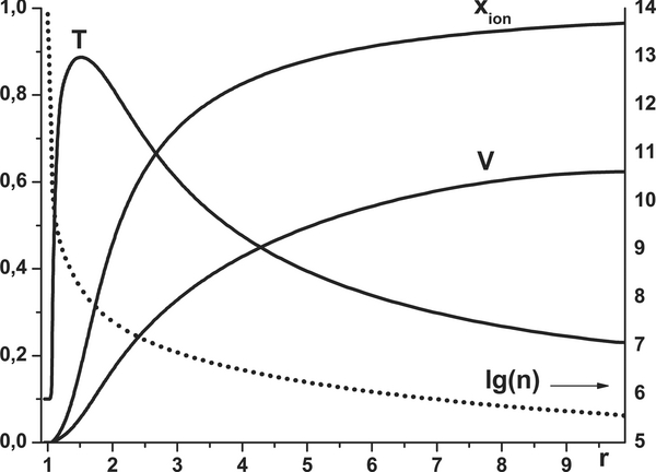
Figure 1 shows the result of a modeling calculation with the typical model parameters summarized in Table 1. The case of an open outer boundary condition was considered. In line with the discussion in Section 3.2, the Lyα reabsorption effects are not important for the studied regime of material free outflow and therefore were not included in the model.
Figure 1. Profile of temperature, velocity, ionization degree (left axis), and density (dotted line, right axis, log scale) in dimensionless units obtained in a calculation with the typical model parameters from Table 1. Download figure:

Table 1. Model Parameters
| Mp | Rp | FXUV (0.05 AU orbit, Sun-analog star) |  |
 |
Outer Boundary Condition |
|---|---|---|---|---|---|
| 0.7 MJ | 1010 cm | 2 × 10³ erg cm−2 s−1 | 1000 K | 10−5 bar | Open |
Download table as: ASCIITypeset image
As can be seen in Figure 1, the maximum temperature realized in the free-outflow regime is about 8500 K and is achieved at a height of about 1.75 · Rp. Then, because of adiabatic cooling, the temperature quickly decreases with height because the XUV heating is not enough to compensate for it once the ionization of the expanding gas takes place. The ionization degree xion = ni/n increases sharply near the temperature maximum, and the velocity of the expanding atmospheric plasma wind driven by the increase in the pressure gradient also increases, mostly at the ionization front. Because the temperature and density quickly decrease with distance, the escaping material reaches supersonic velocity at a distance of about 6 · Rp.
A comparison of the obtained results with the outcomes of the closest (in the sense of model parameters and simulation conditions) model by Koskinen et al. (2013) reveals that, in spite of general (phenomenological) agreement, the models show some nonprincipal difference in specific physical quantities. These may be attributed to the slightly different values of XUV flux used in the modeling simulations, which result in different heating rates qXUV = na〈(EXUV − Eion)σXUVFXUV〉 in Equations (4) (and (11) realized in the course of modeling, and to different net and heating efficiencies. In particular, our model gives a slightly higher density and a bit smaller velocity with a slightly smaller (than by Koskinen et al. 2013) maximum XUV heating rate:  .
.
The calculation of mass loss rate  yields the value 7 · 1010 g s−1, which is by a factor of almost two larger than that predicted with the model by Koskinen et al. (2013). However, the mass loss rates become practically equal if we take the same net efficiency,
  , as that used by Koskinen et al. (2013).
The most significant difference between our model results and those of Koskinen et al. (2013) concerns the predicted maximum temperature, which in our case is 3500 K less. One of the reasons is that Koskinen et al. (2013) use a Lyα cooling reduced by a factor of 0.1. Switching off the Lyα cooling in our model reduces the difference down to 2500 K.
Regardless of the maximum temperature, the value of pressure-averaged temperature
over the distance interval from Rp to 3Rp, which is used in Koskinen et al. (2013) as a measure of a possible transit effect of a planet, in the case of our model is 6000 K. That is rather close to the temperature range of 6200–7800 K reported in Koskinen et al. (2013).
The behavior of the temperature and density of the expanding planetary atmosphere as parametric functions of pressure in the deep region of dense thermosphere layers near the inner boundary, obtained by solving numerically the model equations, is shown in Figure 2. The position of the inner boundary itself in this study was taken slightly (a few percent) below the level of r = 1 (in units of Rp). Note that temperature smoothly approaches the base (inner boundary) temperature To = 0.1 (in units of Figure 2. Temperature and velocity in dimensionless units as functions of pressure at the inner boundary in the thermosphere. Dotted line: analytic solution defined with Equations (16) and (17). Download figure: ), and velocity decreases down to negligibly small values.
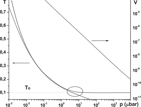
To understand the nature of the obtained numerical result, let us compare it with a simple analytical solution. Close to the inner boundary, in the dense layers of the thermosphere where the velocity is rather small, we can ignore inertial terms and ionization in the momentum Equation (3). Then, the barometric density profile n(r) = n0 exp(− r/H(T, r)) with the local scale height of H(T, r) = r2kT/(GmMp) is an approximate solution of Equation (3), which under the above-mentioned conditions has the following form:
We assume that XUV absorption takes place in a thin layer near r ≈ Rp with very large column densities NL so that σXUVNL ≈ σXUVnH ≫ 1, and it is balanced by adiabatic expansion.
Then, from the energy balance Equation (4) (or (11)) in a quasi-stationary state, using the approximation Equation (7) taken at NL ≫ 1, assuming as a zero-order approximation the barometric density distribution with the scale height H(T, r), and expressing r2Vr in terms of mass loss rate  , we obtain an approximate relation between temperature and density in the vicinity of the inner boundary:
where EF = εXUV/(0.21.2 · tXUV), To is the inner boundary temperature measured in units of  , and
, and  is the local scale height in the vicinity of the inner boundary. In these calculations we continue using tXUV ≈ 6 hr and εXUV ≈ 2.7eV, which correspond to the stellar XUV flux expected at 0.05 AU orbit around a Sun-analog star.
Solution of the barometric Equation (15), with Equation (16) taken into account, yields
The starting point rmin of the solution is determined from Equation (16) by taking T = To and n = no. The maximum pressure (or density, i.e.,  ) up to which solution Equation (17) is valid follows from the right-hand side of Equation (16) with const = 1:

The term in brackets in Equation (18) is approximately a ratio of energy delivered by XUV to energy removed by the expanding material flow, if each particle has energy  . Because the material escape is almost energy limited and the particle energy is 10 times higher than
  , the term in brackets is about 20–30. This means that the maximum pressure is much larger than that at the layer with a density of 1/σXUVHo where a significant portion of XUV is absorbed. Typical hot Jupiter conditions in this case yield an estimate for pressure of pmax ∼ 10 μbar.
The analytic solution Equation (17) expressed by means of Equation (16) as a function of pressure is shown in Figure 2. The value pmax = 10μbar corresponds well to the point (marked by an ellipse) where the numerical solution, approaching the inner boundary level, begins to deviate significantly from the analytical solution of Equation (16). Note that in this region the velocity is already very small. At larger pressures, corresponding to deeper atmospheric layers, the considered model solution is governed more by numerical factors, such as the small viscosity (η = 10−5 in dimensionless units) introduced into Equation (3) for stability reasons. At such very large pressures and so deep in the thermosphere, the hydrogen chemistry, molecular and eddy diffusion are probably more important than the adiabatic cooling considered in this example.
5.3. Planetary Atmosphere Mass Loss: Influence of the Inner Boundary Position and XUV Flux
To investigate how the inner boundary location may influence the obtained numerical results regarding the escape of hot Jupiter atmospheric material and to verify the possibility of neglecting the effects of infrared cooling by  at the base of the thermosphere (as presently assumed), we performed a series of dedicated calculations and present their outcome below.
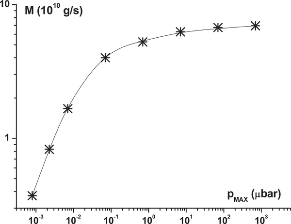
Figure 3 shows a dependence of the simulated mass loss rate on a value of fixed pressure Figure 3. Mass loss rate as a function of the inner boundary pressure Download figure: at the inner boundary, or rather on the position of the inner boundary relative to the fixed distribution Equation (13). One can see that for
 less than psat ∼ 1 μbar the escaping flow is strongly affected by a particular value of the inner boundary pressure
 . Such a dependence of the numerical solution on the inner boundary condition (i.e., on the location of the inner boundary of the simulation box) has been referred to in several previous studies (e.g., Trammell et al. 2011; Adams 2011), where proportionality of the mass loss rate to the boundary pressure was assumed as an input condition. One can see from Figure 3 that, for
  higher than psat ∼ 1μbar, the influence of the inner boundary pressure on the mass loss rate becomes less significant.
 .
.
As to the behavior of other physical quantities in the model, we find that between the cases of  and
and  the material density at distances of a few Rp varies by a factor of two, whereas the location of the temperature maximum for
  shifts by ∼0.3 Rp to smaller heights.
The choice of a particular maximum pressure at the inner boundary is also related to the depth of absorption of XUV photons. The absorption parameter σ(ε) · NL for a photon of given energy ε = hν can be estimated as
Therefore, fixing the thermosphere inner boundary (i.e., depth) at the level of  means that photons with energy higher than ε > 20 · Eion, which correspond approximately to wavelengths shorter than 5 nm, will be excluded from the consideration. Such a restriction would limit the generality of the model.
The discovered mass loss "saturation" effect for sufficiently large inner boundary pressures ( ) is related to a rather weak (for large
  ) dependence of the obtained numerical solution on the base temperature
  . In particular, the variation of
  from 750 K to 1500 K results in a change in the mass loss rate
  by only 14%.
Figure 4 shows the dependence of the mass loss rate on the intensity of XUV radiation of a Sun-like star illuminating the planet (full analog of HD 209458b), expressed in terms of the orbital distance to the star. It has a power-law character. The fact that the increase of the mass loss rate with decreasing distance is very close to R−2 enables one to draw a conclusion on the proportionality between the mass loss rate and the XUV flux. Similar behavior has been reported in a number of papers (e.g., Lammer et al. 2003; Garcia Muñoz 2007).
Figure 4. Dependence of mass loss rate on XUV flux expressed as an orbital distance of a planet to a Sun-like star. The straight line corresponds to R−2. Download figure:
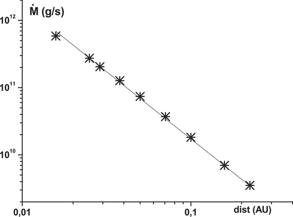
For a Jupiter-type planet at an orbital distance below 0.02 AU near a Sun-like star, the tidal forces and Roche lobe effects, which are not included in our model, become important (Garcia Muñoz 2007; Penz et al. 2008; Erkaev et al. 2007). Therefore, we restrict the considered range of orbital distances by 0.02 AU. To justify the omission of a tidal force, a test calculation was performed for a tidally locked system with the gravity potential in the equatorial plane of mGMp/r(1 + 1/2(r/rL)3), where rL is a distance to the Lagrange point, which for the considered hot Jupiter (HD 209458b) system is rL ≈ 4.6. It was found that the tidal force increases the escape velocity (on the day side of the planet). However, the mass loss rate increases only by 10% and the maximum temperature decreases by only 10%. Therefore, it may be concluded that within the above assumptions the main results of our study are not strongly affected by the inclusion of a tidal force, though it should be taken into account for a complete model of the HD 209458b system (after all of the major effects are properly studied and understood). At the same time, because the main goal of this paper is to build a comprehensive (1D) self-consistent model of a hot Jupiter's upper atmosphere escape for its further generalization to the case of a magnetized planet, without the inclusion of tidal force the role of other material escape drivers and their mutual relation becomes more clear and easy to understand.
5.4. Accounting for the Infrared Cooling Effect
To study the role of the infrared cooling effect in our computations, we followed the approach of Penz et al. (2008) and included the term −naCir in the right-hand side of Equation (4). The taken coefficient Cir = 0.05 K/s approximately corresponds to the  cooling rate reported in Yelle (2004) and García Muñoz (2007).
The  is produced in reactions that involve ionized molecular hydrogen
  in the region where H2 is the dominant species instead of atomic hydrogen. To take this fact into account and restrict the infrared cooling by layers populated by molecular hydrogen, we included reactions of molecular hydrogen dissociation and association, H2 + M↔2H + M, with the rates provided in Yelle (2004) and García Muñoz (2007). Assuming a local balance between H2 and H as determined by the rates of association and dissociation, the relation between species is given by

In the presence of H2 the energy Equation (4) should be modified. At short wavelengths the cross section of XUV absorption by H2 is about 2.5 times larger than that for H. Without making a big error we can put it to be twice larger, that is, the same cross section as for H but for two hydrogen atoms comprising the hydrogen molecule. Finally, the heating term in Equation (4) may be modified corresponding to  . Therefore, in the infrared cooling term −naCir, instead of na we use the sum density,
  . After combining the momentum equations for H2 and H, the momentum equation can also be expressed in terms of the sum density nHΣ and average mass
  :
:
This equation replaces Equation (3) in the considered set of model equations. The average mass  can be expressed through sum density nHΣ using Equation (19).
The corresponding energy density rates for XUV absorption, advection, as well as adiabatic and radiation cooling obtained by solving the modified equations of the model are shown in Figure 5. With the inclusion of infrared cooling Cir, the peak XUV absorption rate is about two times larger than in the calculation presented in Figure 1. This happens because of the deeper penetration of XUV that is due to the generally smaller column density.
Figure 5. Spatial dependencies of XUV absorption rate (thick solid line), advection and adiabatic cooling rate (thin solid line), and radiative cooling rate due to infrared and Lyα emission (dotted line). Download figure:

Note that radiative cooling consists of an infrared part at low temperatures and a Lyα part at sufficiently high temperatures. The maximum infrared cooling rate reaches the maximum XUV heating rate, and both have values slightly larger than 10−7 erg · cm-3 · s−1, which agrees well with the results of Yelle (2004). The value of pressure at this maximum is about 0.07 μbar. The transition from molecular to atomic hydrogen occurs at a slightly larger height, where a pressure of 0.015 μbar and temperature of about 2000 K are realized. One can see that close to the conventional planet surface, i.e., r = 1 (in units of Rp), infrared cooling clearly dominates. Then, after some short space interval (∼0.05Rp), the Lyα radiation becomes an efficient coolant. Finally, at heights above 1.5 Rp only the adiabatic and advection cooling counteract the XUV heating.
The spatial distribution profiles of the main physical quantities obtained in the course of the calculations including the effects of H2 chemistry and Figure 6. Profiles of temperature, velocity, ionization degree (left axis), and density (dotted line, right axis, log scale) in dimensionless units obtained in a calculation that included H2 chemistry and infrared cooling by Download figure: cooling are shown in Figure 6. A comparison of these results with those presented in Figure 1 reveals that accounting for the infrared cooling effects in the deep layers does not lead to any principal difference in the system behavior. Accounting for the
  cooling effect as ∝nHΣCir leads to a reduction of the material escape rate of about two times. Variation of the Cir value by an order of magnitude results only in a moderate (about a factor of 1.7) change in the mass loss rate. Thus, the effect of
  cooling has been estimated more or less robustly. This result differs from that of Penz et al. (2008), where no influence of infrared cooling was reported. In that respect we note that, in spite of the peak cooling rate in our case and in Penz et al. (2008) being the same, the XUV heating rate in Penz et al. (2008) is about an order of magnitude larger.
 for the model parameters from Table 1.
5.5. Material Ionization as a Distributed Acceleration Factor
Here we would like to demonstrate the performance of the above-discussed (Section 3.1) effect of the "ionization boost" (due to the contribution of the electron and ion pressure gradients) in the increase of the atmospheric material outflow speed.
It follows from the integration of Equation (3) over r (from the planet surface to infinity) that the term with the electron pressure gives a positive input to the kinetic energy of the expanding flow. The electron density increases with the radial distance over the integration interval from ne = 0 at r = Rp up to some maximum value and then again falls to zero, and the total number density of hydrogen n monotonically decreases with distance. Because of that, two areas can be distinguished depending on the radial distance r: (1) the area of increasing electron pressure (closer to the planet) where the pressure gradient acts as a decelerating factor on the plasma flow, and (2) the outer area of decreasing pressure where the electron pressure gradient accelerates the expanding plasma flow. Because the total density n decreases exponentially fast with distance, and the location of maximum of electron pressure is spatially close to that of the maximum temperature, the overall contribution of the electron pressure gradient term in the flow kinetic energy can be estimated as
The effect of acceleration of the escaping wind by the additional pressure gradient of the ionized gas is illustrated in Figure 7, where besides the typical free-outflow solution (the same as in Figure 1), the calculations without ionization and with zero electron pressure are shown. In the limiting case without ionization, the XUV radiation equally heats the whole volume of gas, resulting in a very large escape velocity and high temperature that continuously increase with distance. The speed of the expanding wind exceeds the adiabatic sonic point Figure 7. Profiles of velocity and temperature in the true case (dotted lines), the zero electron pressure case (thick lines), and the no-ionization case (thin lines). Download figure: at about 7.3 Rp. In another limiting case, shown in Figure 7, the effect of material ionization is included. This results in the spatial dependence of XUV heating and its strong decrease at heights beyond several Rp. At the same time, the electron pressure in this limiting case (i.e., the ionization boost) is set to zero, so the effect of the additional pressure gradient of the ionized gas is artificially ignored. The resulting flow velocity in this case is essentially smaller than that in the true case, and it never reaches the sound speed values, while the overall mass loss is 1.5 times smaller. Contrary to these limiting cases, the true case, with the effects of ionization and the additional pressure gradient of the ionized gas (electron pressure) properly taken into account, is characterized by an increase in outflow velocity, which reaches a sonic point at the distance of 6.25 Rp. Note that because of the different spatial distributions of temperature in the cases considered here, the corresponding density profiles are also essentially different.
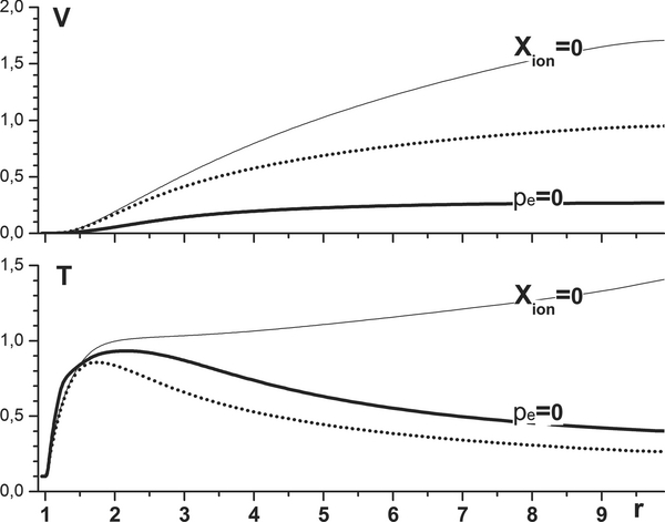
The comparison of the limiting cases presented in Figure 7 enables one to conclude that the effect of the ionization boost is essentially important in the case of a hot Jupiter's expanding atmosphere. It appears to be a major mechanism that compensates to a certain degree for the decelerating action of adiabatic cooling and provides the necessary additional propulsion force to support the free-outflow regime of atmosphere expansion.
Inclusion of the tidal force effects in the comparative study of the "ionization boost" slightly but not principally affects the results of the modeling. In particular, whereas in the case without the tidal force the effect of the "ionization boost" at r = 8 Rp causes an increase in the escape velocity of ΔV ≈ 0.5 (see Figure 7), the inclusion of the tidal force under the same other conditions results in ΔV ≈ 0.4.
It should be noted that electron pressure acts primarily on ions. In the outer, highly ionized layers of the expanding atmosphere, where the electron pressure gradient acts as an accelerating force, the ions naturally appear as a major mass-contributing component. As to the inner regions populated by partially ionized plasma, it was shown by Guo (2011) that because of fast charge exchange the added momentum of ions is effectively transferred to atoms.
5.6. Restricted-flow Regime of a Hot Jupiter's Atmosphere Expansion
When the closed condition is applied at the outer boundary of the simulation box, the expanding atmospheric material flow gradually decays until a steady state with an almost zero flux through the outer boundary is achieved. This situation corresponds to the suppressed- or restricted-flow regime. Because of the absence of adiabatic cooling in this case, the energy-balance condition is provided for due to Lyα emission. This is true everywhere except in a cold, nonionized, and dense thermosphere with a temperature of several thousand K and less. In reality, in the case of a complete absence of material escape, a solution with a temperature at the inner boundary on the order of 1000 K, provided only by Lyα cooling, is not possible. Therefore, in our numerical model we allow a small outflow velocity at the outer boundary such that the corresponding small flow in the dense thermosphere can sustain an energy balance with the XUV heating. Under these circumstances, the material escape rate is proportional to the allowed fixed-outflow velocity at the outer boundary. It is worth, in that respect, comparing the different temperature profiles realized for different outflow velocities.
Figure 8 shows the temperature profiles obtained for different values of the outer boundary outflow velocity. With a series of subsequent simulation runs we found that for Vout < 0.1 km s-1 the solution does not depend on the outflow velocity Vout at the outer boundary any more. The maximum value of the velocity achieved inside the simulation box is about two to three times larger than the outer boundary outflow velocity, but it still remains rather small, Vmax < 0.25 km s-1. At a fixed outer boundary velocity of Vout = 0.1 km s-1, the mass loss rate is 3.5 times smaller than in the case of free outflow (i.e., open outer boundary).
Figure 8. Temperature profile in the case of a restricted-flow regime for different fixed outflow velocities: 0.1 (thin solid line), 0.03 (dashed), 0.01 (thick solid), and 0.003 (dotted). Download figure:

It can be seen in Figure 8 that the material temperature grows much faster near the planet surface as compared to the case of an open outer boundary condition. The temperature grows continuously over large distances because the adiabatic cooling does not work in this case, except in only a restricted region at r ⩽ 1.15 Rp close to the planet surface. The pressure-averaged temperature (see Equation (14)) in the interval of heights Rp ⩽ r ⩽ 3 Rp is about 9000 K. This leads to the formation around a planet of a gas envelope that is several times (up to an order of magnitude) denser and somewhat hotter, as compared to the case of a free-outflow regime.
As already pointed out, the temperature in the case of a restricted-flow regime depends on the efficiency of Lyα cooling. In view of the fact that deep near the planet surface the atmospheric gas is optically thick for Lyα, it is important to also check for the possible influence of Lyα reabsorption (included in Equation (11)). It becomes important when the number of Lyα photons is sufficiently large:  .
.
This estimation follows from Equation (12) after an approximation of spatial derivatives as Figure 9. Temperature and density distributions in the case when Lyα reabsorption is included in the model (thick solid lines) and without it (dashed lines). A closed condition (i.e., a restricted-flow regime) is applied at the outer boundary in both cases. For comparison, the dotted line shows the density distribution in the case of the open (i.e., free-outflow regime) outer boundary condition. Download figure: . For the conditions of restricted flow, the reabsorption affects the Lyα cooling rate at heights below 2 Rp (Figure 9). Figure 9 shows the result of a model calculation with a relatively high Lyα absorption cross section of σLα ∼ 10−14T-1/2 cm2.
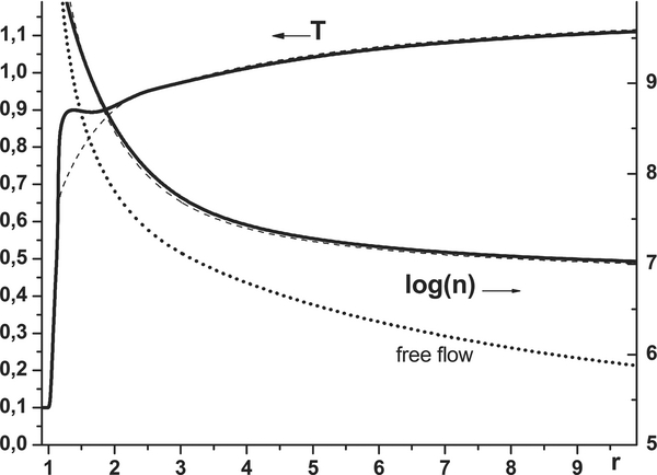
As expected, because of strong reabsorption and an established balance between hydrogen excitation and deexcitation that diminishes the efficiency of cooling, the temperature visibly increases at distances below 2 Rp. The maximum increase in temperature as compared to the case without Lyα reabsorption is about 1500 K. Farther from the planet, the effect of Lyα reabsorption decreases, and for r > 2.5 Rp it becomes negligible. As to the influence of Lyα reabsorption on the gas density at distances up to several Rp, i.e., inside the dead-zone region that might be formed in the presence of a magnetic field, as can be seen in Figure 9, such an influence is rather small and practically undistinguishable in the numerical calculation result. Therefore, depending on the purpose of the particular numerical simulation, in some cases the effect of Lyα reabsorption can be neglected, despite its obvious influence on the temperature of gas close to the planet.
Figure 9 also allows one to compare the density distributions realized in the cases of open and closed outer-boundary conditions, i.e., in the free-outflow and restricted-flow regimes, which may correspond, for example, to the "wind" and "dead" zones of a hot Jupiter magnetosphere (Trammell et al. 2011; Khodachenko et al. 2012). In particular, the plasma density in the case of a restricted-flow regime is up to an order of magnitude higher than in the case of free outflow.
Based on the obtained numerical solutions, it is possible to estimate the strength of a hot Jupiter's magnetic field needed to affect and confine the hot gaseous envelope around the planet, energized by the stellar XUV. For this purpose we check the spatial behavior of the plasma beta 8πnT/B2 in the equatorial plane for different values of magnetic field at r = Rp, assuming for the sake of being definitive an undisturbed magnetic dipole field geometry and a quasi-stationary restricted-flow regime. The result is presented in Figure 10, which in particular shows that surface fields larger than 1 G should strongly affect the plasma outflow. The area of strongest magnetic control is located near 2 Rp, whereas the overall size of the magnetic field–dominated region may reach, depending on the field strength, up to several Rp. Note that because of the steep density increase close to the planet surface, thermal pressure exceeds magnetic pressure even for very large surface fields.
Figure 10. Spatial behavior of plasma thermal beta for different strengths of magnetic field at the planet's surface. Download figure:

Another interesting issue concerns the flow above the dipole poles. As is well known, if plasma moves along the magnetic field lines in a strong dipole field, the divergence of material flux (guided by the magnetic field lines) at the pole regions is larger than that in the case of a spherically isotropic expansion. Because adiabatic cooling is crucial for sustaining the temperature of the expanding material, a certain reduction of the temperature and escape velocity in the polar regions, as compared to the isotropic expansion case, may be expected. This effect is demonstrated in Figure 11, which shows the outcome of our 1D HD simulation with an artificially increased ("cubic") divergence term as ∂V/∂r + 3V/r (analogous to the divergence of a dipolar magnetic field in polar regions), taken instead of the true divergence term divV = ∂V/∂r + 2V/r, which corresponds to an isotropic spherically symmetric expansion. Justification for such a substitution based on the dipole field geometry can be found, for example, in Trammell et al. (2011). One can see in Figure 11 that the outflow velocity and density in the case of increased divergence are significantly smaller. The maximum temperature realized in the case of inflated flow is ∼1000 K lower than that for the spherically symmetric isotropic flow. The sonic point is reached at about 8 Rp and farther than in the equatorial case, contrary to expectations.
Figure 11. Velocity and density in the case of an artificially increased ("cubic") divergence (solid lines) in comparison with the true divergence case (dashed lines). Download figure:
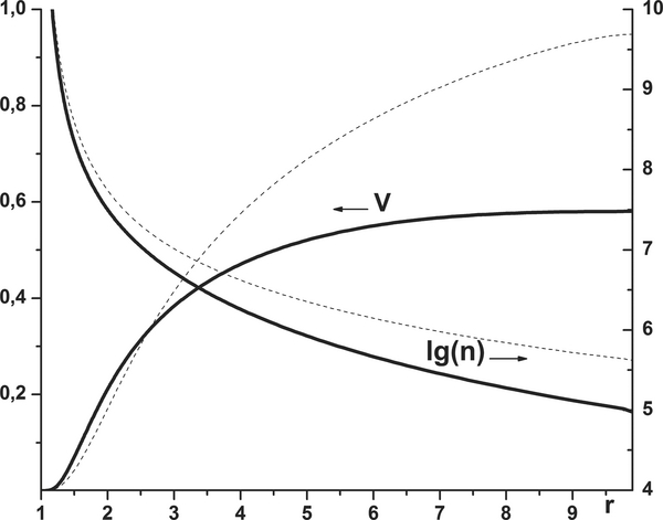
6. DISCUSSION AND CONCLUSIONS
We investigated the formation and escape regimes of a hot plasma envelope of a Jupiter-type exoplanet created by XUV heating of the planetary hydrogen atmosphere while taking into account the processes of radiation transfer (i.e., excitation/deexcitation), ionization/recombination, and adiabatic cooling of the atmospheric gas. Our study confirmed the results reported in a number of previous works dedicated, as in the present paper, mostly to the exoplanet HD 209458b (Yelle 2004; García Muñoz 2007; Guo 2011, 2013; Koskinen et al. 2010, 2013) and revealed that a hot Jupiter plasma envelope under the typical conditions of an orbital distance 0.05 AU around a Sun-type star should be rather hot, but with not very fast hydrodynamic escape, resulting in mass loss rates of about (4 − 7) · 1010 g s-1. The escaping material flow becomes supersonic at distances of about 10 planetary radii.
Note that, being interested in the pure thermal escape of a hot Jupiter upper atmosphere caused only by stellar radiation factors (i.e., material XUV heating and ionization), we did not include the effects of the stellar–planetary gravitational interaction. On the other hand, from the dedicated studies (Penz et al. 2008; Erkaev et al. 2007, 2013), it is known that in a system like that of HD 209458b the location of the L1 point is at about 4.3 Rp. This means that the effects of gravitational material escaping because of gas expansion beyond the Hill sphere add to the pure thermal mass loss and should be properly included in a more complete model. At the same time, preliminary estimates provided in the present paper (Figure 10) reveal that the intrinsic magnetic field may strongly influence the motion of the escaping planetary plasma up to the distances comparable with L1 in the HD 209458b system. In this case the role of the gravitational escape effects will be strongly diminished, whereas the dominating magnetic field will control the process of the mass loss.
To evaluate the physical drivers of the escape and the parameters of the created hot plasma envelope around the planet, we checked the influence of various processes, such as infrared cooling by  molecules in the deep and cold layers of the planetary thermosphere, emission and reabsorption of Lyα photons, and boundary and the geometry conditions that may reflect different kinds of interaction with the planetary magnetic field.
Having in mind the primary goal of the 1D HD numerical modeling presented in this paper, as a first step in our two-step modeling approach aimed at understanding first the hydrodynamic behavior of the expanding nonmagnetized upper atmosphere of a giant exoplanet, significant attention was paid to the investigation of different types of boundary conditions and their influence on the achieved material escape regimes. Based on this understanding, the next step (MHD modeling) with the consequent inclusion of the planetary magnetic field and its relevant effects can be done in a more comprehensive and justified way. Moreover, several general conclusions regarding the influence of a magnetic field on the plasma distributions, flows, and temperature regimes were already possible in the present HD simulations, based on the results obtained for different types of inner and outer boundary conditions.
It was found that because of the ability of the short-wavelength photons to penetrate deeper into the atmosphere, the high-energy part of the XUV spectrum, as a heater of the deep and dense layers of the thermosphere, plays an important role in the formation of a hot plasma envelope around the planet. This is directly related to the value of maximum pressure implied at the inner boundary of the planet. Using the proxy model of spectrally integrated solar XUV flux, we derived a simple analytical estimate for the maximum pressure (Equation (18)) up to which XUV heating can be balanced by adiabatic cooling for the given base temperature of the atmosphere and mass loss rate. For the typical parameters of HD 209458b, this pressure is ∼10 μbar, i.e., higher than that used in previous models of the planet. Note that the velocity of escaping gas at the height where this pressure is realized in the atmosphere is negligibly small as compared to the thermal speed, and the XUV spectral cutoff is around the wavelength of 2.5 nm. It was also demonstrated with a series of test simulations that the inner boundary of the simulation box located at the heights of lower pressures produces proportionally smaller escape rates, whereas the boundary at larger pressures gives approximately the same results.
At the pressure values used at the inner boundary, the hydrogen is present mostly in a molecular form, and such species as  may provide an efficient cooling effect by infrared radiation. By incorporation of these factors into the model we found that the hydrogen chemistry at the base of the thermosphere might change the parameters of the formed hot extended plasma envelope and result in reduction of the material escape rate by a factor of about two.
In the present work we also reached a deeper insight into the mechanism of formation of the escaping planetary wind. As is known from stellar wind studies, a supersonic flow of escaping material has to be supported by a mechanism of additional heating/energizing, which operates in the distance range where the flow gains its greatest velocity. Various mechanisms of wave heating are traditionally referred to for the stellar winds in that regard, although the exact process remains unknown. In the case of a hot Jupiter, it appears that the XUV heating of atmospheric gas alone is not enough to balance the adiabatic cooling at distances of several planetary radii because gas becomes ionized and the radiation absorption decreases at heights >3 Rp. However, the same effect of gas ionization, which reduces the efficiency of XUV heating, plays the important role of a booster of the escaping wind because of the buildup of an additional electron pressure gradient force. The thermal pressure almost doubles at the ionization front because of the appearance of additional electron pressure, which contributes to the acceleration of the escaping partially ionized plasma flow. This effect means that part of the absorbed stellar XUV energy is stored in the thermal energy of electrons and is then converted into the kinetic energy of the expanding plasma flow. In that respect, a self-consistent account of the processes of gas ionization and recombination is crucial for the correct calculation of planetary atmospheric material escape. A simple use of the prescribed or fixed ionization ratios may lead to unrealistic and erroneous results in that respect.
We investigated two types of HD solutions that represent two basic regimes (restricted flow and free outflow) of the expanding gaseous envelope of a giant exoplanet heated by stellar XUV. In fact, both regimes can be realized in the same physical system, depending only on the type of outer boundary condition (closed or open), which may in their turn be a consequence of the specific action of the planetary magnetic field.
In the free-outflow regime the adiabatic cooling alone provides an efficient balance to XUV heating. It dominates over the radiation cooling everywhere except at the base of the dense and cold thermosphere, where infrared radiation is more efficient. Lyα radiation cooling may compete with adiabatic cooling only in a thin layer around the temperature maximum and, as we have found out, only if the mass loss rate is below 5 × 10¹⁰ g s-1. It was found that at orbital distances from 0.25 to 0.1 AU, where the effects of stellar gravitation may be still unimportant, the mass loss rate is mainly defined by the expansion and escape of the hot planetary atmospheric material, and it is proportional to the stellar XUV flux.
The kinetic mV2/2 and thermal 3kT/2 energies per particle in a fully ionized escaping gas are an order of magnitude smaller than the stored ionization energy Eion. A part comparable with Eion in the energy budget is the energy of particles (Eg = 8.6 eV) that exit the gravitational bounding of the planet. Because the energy deposited in the system by the XUV flux illuminating the planet is removed mainly by the expanding gas outflow (except for an inessential part lost via Lyα photons), and this was confirmed to be true by the performed numerical calculations, the atmospheric mass loss can be estimated as  . This value for ηnet = 50% is just about 14% less than the
  obtained in the course of the numerical simulations. Note that the heating efficiency ηh is not included in these estimations because the energy spent by the ionization of neutral atmospheric gas constitutes the major portion of the whole absorbed energy. This estimate indicates that in the range of the considered stellar–planetary parameters and XUV fluxes the mass loss is indeed energy limited, as was found in a number of other models (Lammer et al. 2003; Erkaev et al. 2007).
In the restricted-flow regime, the XUV heating is balanced by gas excitation and radiation of infrared and Lyα photons. However, the infrared and Lyα cooling act only at certain restricted and nonoverlapping temperature ranges that correspond to particular regions in the atmosphere. As result, the layers with temperatures between 2000 K and 7000 K cannot be effectively cooled by radiation. Because of that, a flow with relatively small, of about 200–300 ms-1, velocities at the outer boundary is built up that provides the necessary additional adiabatic cooling. Mass conservation requires that the material is either removed through the outer boundary or is settled in a kind of zonal convection.
Another specific detail of the restricted-flow solution that we investigated is Lyα reabsorption. For the cross section of about 10−15 to 10−14 cm2, the atmospheric gas of the considered giant planet HD 209458b is everywhere optically thick for Lyα photons. The reabsorption leads to an increase in the population of excited hydrogen atoms and results in a decrease of Lyα cooling. The numerical solution that treats Lyα radiation transfer in a diffusion approximation shows that the optical thickness of the gaseous envelope leads to an increase in temperature of about 1000 K at distances below 2 Rp. At the same time, at larger distances the temperature and density remain nearly the same as in the case without inclusion of Lyα reabsorption.
Finally, based on the simulated escaping atmosphere of HD 209458b, we find that the intrinsic planetary magnetic field, which may have at the planetary surface a value higher than 1 G, may certainly affect the material flow and result in formation of a "dead" zone of stagnated plasma in the equatorial plane around the planet. In the magnetic polar regions, the material escape rate might be severely diminished due to stronger divergence of the magnetic dipole field lines, as compared to the spherically isotropic case. That results in a stronger adiabatic cooling.
This work was supported by SB RAS Research Program grant II.8.1.4, RFBR grants 09-08-00970, 12-02-00367, and 14-29-06036, and OFN RAS Research Program No. 22. M.L.K., H.L., and K.G.K. acknowledge the projects P25587-N27, S11606-N16, and S11607-N16 of the Austrian Science Foundation (FWF). The authors are thankful to EU FP7 project IMPEx (No. 262863) for support of numerical modeling work and providing a collaborative environment for research and communication. The authors also thank the International Space Science Institute (ISSI) in Bern, and the ISSI team "Characterizing stellar- and exoplanetary environments."