


ABSTRACT
We describe a new method (Poisson probability method, PPM) to search for high-redshift galaxy clusters and groups by using photometric redshift information and galaxy number counts. The method relies on Poisson statistics and is primarily introduced to search for megaparsec-scale environments around a specific beacon. The PPM is tailored to both the properties of the FR I radio galaxies in the Chiaberge et al. sample, which are selected within the COSMOS survey, and to the specific data set used. We test the efficiency of our method of searching for cluster candidates against simulations. Two different approaches are adopted. (1) We use two z ∼ 1 X-ray detected cluster candidates found in the COSMOS survey and we shift them to higher redshift up to z = 2. We find that the PPM detects the cluster candidates up to z = 1.5, and it correctly estimates both the redshift and size of the two clusters. (2) We simulate spherically symmetric clusters of different size and richness, and we locate them at different redshifts (i.e., z = 1.0, 1.5, and 2.0) in the COSMOS field. We find that the PPM detects the simulated clusters within the considered redshift range with a statistical 1σ redshift accuracy of ∼0.05. The PPM is an efficient alternative method for high-redshift cluster searches that may also be applied to both present and future wide field surveys such as SDSS Stripe 82, LSST, and Euclid. Accurate photometric redshifts and a survey depth similar or better than that of COSMOS (e.g., I < 25) are required.
Export citation and abstract BibTeX RIS
1. INTRODUCTION
Clusters of galaxies are among the most massive large-scale structures in the universe. They form from gravitational collapse of matter concentrations induced by perturbations of the primordial density field (Peebles 1993; Peacock 1999). Galaxy clusters have been extensively studied to understand how large-scale structures form and evolve during cosmic time, from galactic to cluster scales (see Kravtsov & Borgani 2012 for a review).
Despite this, the properties of the cluster galaxy population and their changes with redshift in terms of galaxy morphologies, types, masses, colors (e.g., Bassett et al. 2013; McIntosh et al. 2014), and star formation content (e.g., Zeimann et al. 2012; Santos et al. 2013; Strazzullo et al. 2013; Gobat et al. 2013; Casasola et al. 2013; Brodwin et al. 2013; Zeimann et al. 2013; Alberts et al. 2014) are still debated, especially at redshifts z ≳ 1.5.
It is also unknown when the intracluster medium (ICM) virializes and starts emitting in X-rays and upscattering the CMB through the Sunyaev–Zel'dovich (SZ) effect (Sunyaev & Zel'dovich 1972). See Rosati et al. (2002) for a review. In general, the formation history of the large-scale structures and the halo assembly history (e.g., Sheth & Tormen 2004; Dalal et al. 2008) are not fully understood.
High-redshift clusters counts are used to constrain cosmological parameters (e.g., Planck Collaboration XX 2013), to test the validity of the ΛCDM scenario and quintessence models (Jee et al. 2011; Mortonson et al. 2011; Benson et al. 2013). Cluster counts are strongly sensitive to the equation of state of the universe, especially at z ≳ 1 (Mohr 2005), when the universe starts accelerating and the dark energy component starts becoming dominant. The SZ effect, weak lensing measurements (Rozo et al. 2010), X-ray scaling relations, and data (Vikhlinin et al. 2009; Mantz et al. 2010) are used to evaluate the mass, the redshift of the clusters, and their mass function. Moreover, high-redshift cluster samples might be used to test the (non-) Gaussianity of the primordial density field and to test alternative theories beyond General Relativity (see Allen et al. 2011; Weinberg et al. 2013 and references therein for a review).
Searching for high-redshift z ≳ 1 galaxy clusters is therefore a fundamental issue of modern astrophysics to assist our understanding of open problems of extra-galactic astrophysics and cosmology from both observational and theoretical perspectives.
An increasing number of high-redshift z ≳ 1 spectroscopic confirmations of cluster candidates have been obtained in the last years. To the best of our knowledge, in the literature there are only 11 spectroscopically confirmed z ≳ 1.5 clusters (Papovich et al. 2010; Fassbender et al. 2011; Nastasi et al. 2011; Santos et al. 2011; Gobat et al. 2011; Brodwin et al. 2011, 2012; Zeimann et al. 2012; Stanford et al. 2012; Muzzin et al. 2013; Newman et al. 2014). Only some of them have estimated masses greater than 1014 M☉. In addition, Tanaka et al. (2013) spectroscopically confirmed a z = 1.6 X-ray emitting group, whose estimated mass is 3.2 × 10¹³ M☉. A z ∼ 1.7 group associated with a z ∼ 8 lensed background galaxy was found by Barone-Nugent et al. (2013).
High-redshift clusters have been searched for using several independent techniques; such as, e.g., those that use X-ray emission (e.g., Cruddace et al. 2002; Böhringer et al. 2004; Henry et al. 2006; Šuhada et al. 2012) or the SZ effect (e.g., Planck Collaboration XXIX 2013; Hasselfield et al. 2013; Reichardt et al. 2013). However, such methods require a minimum mass and are rapidly insensitive to detecting z ≳ 1.2 clusters (see, e.g., discussion in Zeimann et al. 2012). This seems to also be true for the SZ effect.
It is commonly accepted that early-type passively evolving galaxies segregate within the cluster core and represent the majority among the galaxy population, at least at redshifts z ≲ 1.4 (e.g., Menci et al. 2008; Tozzi et al. 2013).
Various methods search for distant clusters by taking advantage of this segregation. Its evidence is observationally suggested by a tight red-sequence relation which early-type galaxies exhibit in the color–magnitude plots. Such high-z searches are therefore based on overdensities of red objects and are commonly performed adopting either optical (Gladders & Yee 2005) or infrared (Papovich 2008) color selection criteria. They find a great number of cluster candidates, even at z ∼ 2 (e.g., Spitler et al. 2012). However, all these methods seem to be less efficient at redshifts z ≳ 1.6. Moreover, such methods require a significant presence of red galaxies. There might be a bias in excluding clusters with a significant amount of star-forming galaxies or, at least, such searches might be biased toward large-scale structures with specific properties in terms of galaxy colors (Scoville et al. 2007a; George et al. 2011).
The red-sequence has been confirmed in clusters and observed to be fairly unevolved up to z = 1.4 (Mei et al. 2009; Rosati et al. 2009; Strazzullo et al. 2010). However, its presence and evolution are still debated at higher redshift. Recent work showed evidence of increasing star formation activity in cluster cores at z ≳ 1.5 (Hilton et al. 2010; Fassbender et al. 2011; Santos et al. 2011).
Several methods use photometric and/or spectroscopic redshifts to search for high-redshift overdensities (Eisenhardt et al. 2008; Knobel et al. 2009, 2012; Adami et al. 2010, 2011; George et al. 2011; Wen & Han 2011; Jian et al. 2014). Similar to the methods outlined above, they are generally less efficient at z ≳ 1.5. This is due to the difficulty of obtaining spectroscopic redshift information for a sufficient number of sources at z > 1, to the significant photometric redshift uncertainties, and to the small number density of objects.
In fact, typical 1σ statistical photometric redshift uncertainties are ∼0.15 at redshifts z = 1.5, while the mean number of galaxies within a redshift bin Δz = 0.3 and a circle of 1 Mpc diameter is ≲ 9 and ≲ 3, at z = 1.5 and z = 2.0, respectively.
Powerful radio galaxies (i.e., FR IIs; Fanaroff & Riley 1974) have been extensively used for high-redshift cluster searches (e.g., Rigby et al. 2014). High-redshift (i.e., z ≳ 2) high-power radio galaxies are frequently hosted in Lyα emitting protoclusters (see Miley & De Breuck 2008 for a review). Recently, Galametz et al. (2012) and Wylezalek et al. (2013) searched for megaparsec-scale structures around high-redshift (i.e., z ≳ 1.2), high-power radio galaxies using an IR color selection (Papovich 2008).
FR I radio galaxies (Fanaroff & Riley 1974) are intrinsically dim and are more difficult to find at high redshifts than the higher-power FR IIs. This has so far limited the environmental study of the high-redshift (z ≳ 1) radio galaxy population to the FR II class only.
However, due to the steepness of the luminosity function, FR I radio galaxies represent the great majority among the radio galaxy population. Furthermore, on the basis of the radio luminosity function, hints of strong evolution have been observationally suggested by previous work (Sadler et al. 2007; Donoso et al. 2009). Their comoving density is expected to reach a maximum around z ∼ 1.0–1.5 according to some theoretical models (e.g., Massardi et al. 2010).
At variance with FR II radio galaxies or other types of active galactic nuclei (AGNs), low-redshift FR Is are typically hosted by undisturbed ellipticals or cD galaxies (Zirbel 1996), which are often associated with the brightest cluster galaxies (BCGs; von der Linden et al. 2007). FR Is are preferentially found locally in dense environments at least at low redshifts (Hill & Lilly 1991; Zirbel 1997; Wing & Blanton 2011). This suggests that FR I radio galaxies might be more effective for high-redshift cluster searches than FR IIs.
Chiaberge et al. (2009, hereinafter C09) derived the first sample of z ∼ 1–2 FR Is within the COSMOS field (Scoville et al. 2007b). Chiaberge et al. (2010) suggested the presence of overdensities around three of their highest redshift sources. Based on galaxy number counts, the authors found that the megaparsec-scale environments of these sources are 4σ denser than the mean COSMOS density. Tundo et al. (2012) searched for X-ray emission in the fields of the radio galaxies of the C09 sample. They took advantage of the Chandra COSMOS field (C-COSMOS). They did not find any evidence for clear diffuse X-ray emission from the surroundings of the radio galaxies. Their stacking analysis suggests that, if present, any X-ray emitting hot gas would have temperatures lower than ∼2–3 keV. Furthermore, Baldi et al. (2013) derived accurate photometric redshifts for each of the sources in the Chiaberge et al. (2009) sample.
The goal of this project is to search for high-redshift clusters or groups using FR I radio galaxies as beacons. In this paper we introduce our newly developed method and we test it against simulations. The method is tailored to the specific properties of the sample (C09) we consider, and it uses photometric redshifts. In a companion paper (Castignani et al. 2014, hereafter Paper II) we apply our method to the C09 sample. We will refer to the sources in the sample using the ID number only, as opposed to the complete name COSMOS-FR I nnn.
In Section 2 we outline the motivations for introducing our new method; in Section 3 we briefly describe our newly developed method. Then we test our method against simulations. In Section 4 we consider two z ∼ 1 clusters, and we test the efficiency of our method to detect them when they are located at different redshifts. In Section 5 we perform similar tests on simulated clusters. In Section 6 we summarize our results and we draw conclusions. In the Appendix we fully describe the details of our method.
Throughout this work we adopt a standard flat ΛCDM cosmology with matter density Ωm = 0.27 and Hubble constant H0 = 71 km s−1 Mpc−1 (Hinshaw et al. 2009). The physical projected distance is fairly constant within the redshift range of our interest, and it varies by ∼5% from z = 1 to z = 2. At redshift z = 1.5, a projected separation of 60 arcsec corresponds to 512 kpc (physical units).
2. MOTIVATIONS FOR A NEW METHOD
As outlined in Section 1, the goal of this work is to introduce a new method to search for high-redshift (z ≳ 1) megaparsec-scale overdensities on the basis of photometric redshifts only. We primarily introduce the method in order to search for groups and clusters in the COSMOS field (Scoville et al. 2007b) around the FR I radio galaxies in the C09 sample. Due to the COSMOS multiwavelength coverage, increasingly accurate photometric redshift determinations have been derived (Mobasher et al. 2007; Ilbert et al. 2009).
Our method is tailored to the specific properties of both the sample and the survey adopted, but it can be also applied to other multiwavelength surveys and samples, if accurate photometric redshift information is available.
Furthermore, the method requires the projected coordinates of fiducial beacons (e.g., in our project we adopt the sample of z ∼ 1–2 radio galaxies). This implies that our method relies on a positional prior, i.e., it is introduced to search for a cluster or group environment around assigned locations in the projected sky. Therefore, it is not properly a method to search blindly for clusters and groups within a given survey, even if it can be possibly applied for such purposes. This strategy is similar to that adopted in George et al. (2011), who associated galaxies with previously selected groups and that adopted in Hao et al. (2010), who searched for clusters around the BCGs.
In this section we briefly discuss the problems that affect methods that search for high-redshift clusters on the basis of number densities, with particular attention to those that use photometric redshifts. Then, we focus on the peculiarities of our sample and the resulting need for introducing a new method to search for high-redshift megaparsec-scale overdensities.
- 1.As pointed out by Scoville et al. (2007a), methods that identify high-redshift structures on the basis of the observed surface densities have to discriminate galaxies at different redshifts, to avoid projection effects. As noted in Eisenhardt et al. (2008), galaxy number counts are more susceptible to projection effects than, for example, the detection of X-ray emission from the ICM. This makes problematic the identification of the structures at different distances along the line of sight.
- 2.Number densities are increasingly small for increasing redshifts, at z ≳ 1. This affects also the deepest sky surveys. For example, the COSMOS field survey has, on average, number densities per unit redshift of ∼25, 10, and 3 counts arcmin−2 dz−1 at redshift z ∼ 1, 1.5, and 2.0, respectively (Ilbert et al. 2009), where only those galaxies with i+ AB magnitudes in the range 21.5 < i+ < 24.5 are considered. These low number counts imply that shot-noise strongly affects any z ∼ 1–2 cluster search based on galaxy number counts and photometric redshifts since megaparsec-scale overdensities are extended and detected over scales of ∼1 arcmin (e.g., Santos et al. 2009), typical of those of cluster cores. In fact, 1 arcmin corresponds to ∼480 kpc at z = 1.
- 3.Typical statistical photometric redshift uncertainties are σz ∼ 0.1–0.2 at redshifts z ∼ 1–2. This applies to surveys such as COSMOS (Ilbert et al. 2009) and CFHTLS (Coupon et al. 2009). Note that a distance of σz = 0.1 along the line of sight corresponds to more than 100 Mpc, which is significantly more than the typical size of large-scale structures in the universe. Therefore, these uncertainties highly affect the line of sight discrimination of real cluster members from the foreground and any attempts to determine cluster membership on the basis of photometric redshifts only.Furthermore, the typical statistical photometric redshift uncertainty increases within the redshift interval of our interest and undergoes a catastrophic failure at z ≳ 1.5 (Ilbert et al. 2009). In fact, photometric and spectroscopic redshift information cannot be easily obtained between z ∼ 1–2 because most of the relevant spectral features fall outside of the instrumental wavelength bands in that redshift range, which is therefore called redshift desert (Steidel & Shapley 2004; Banerji et al. 2011).
- 4.Megaparsec-scale overdensities might undergo significant evolution between z ∼ 1–2. Their structure and number density might significantly change with cosmic time. In fact, diffuse protoclusters with star-forming galaxies have been in fact found at redshifts higher than z ∼ 2.0 (Steidel et al. 2000; Venemans et al. 2007; Capak et al. 2011).
Methods that search for high-redshift groups or galaxy clusters that are based on optical number counts and photometric redshifts have to carefully identify the different megaparsec-scale structures that are present along the line of sight, in order to avoid projection effects.
Most of the existing methods, such as those that are based on wavelets, Friends-of-Friends algorithms, peak finding methods, Delaunay–Voronoi tessellations, and adaptive kernel (see, e.g., Ebeling & Wiedenmann 1993; Postman et al. 1996; Scoville et al. 2007a; Eisenhardt et al. 2008) that search for high-redshift clusters on the basis of number counts and redshifts are very efficient at z ≲ 1.5, but show reduced efficiency at higher redshifts because of the abovementioned problems.
All these methods are based on the two-dimensional (2D) surface density more than on the three-dimensional (3D) number density. As noted in Scoville et al. (2013), considering the 3D number density would require a more accurate photometric redshift information. All the abovementioned methods characterize the projected space with a high accuracy, in order to identify megaparsec-scale structures of different scales. However, such a detailed multi-scale projected space analysis implies that establishing whether multiple overdensity peaks in the 2D projected density field are part of a single larger structure in practice becomes extremely difficult and subjective (Scoville et al. 2013). For this reason, previous studies are not always able to provide galaxy cluster and group candidate catalogs (Scoville et al. 2013). Therefore, we will introduce a less sophisticated but flexible method to overcome to these limitations.
Furthermore, high photometric redshift uncertainties do not allow us to consider the 3D number density. Therefore, we consider the 2D surface density and the redshift information separately. In order to overcome the problems listed above, a detailed distance discrimination based on photometric redshifts is therefore required. As we show in the following this can be achieved to the detriment of a less detailed tessellation of the projected space.
3. THE POISSON PROBABILITY METHOD (PPM)
Our method is based on galaxy number counts and photometric redshifts. It consists in searching for a dense environment around a given location in the sky. Concerning our specific goal to search for cluster environments around the FR Is in the C09 sample, we will adopt the photometric redshift information for the galaxies in the COSMOS field as given in the Ilbert et al. (2009) catalog. Limiting the sample to only FR Is, we consider their recently estimated photometric redshifts from Baldi et al. (2013), when spectroscopic redshifts from the zCOSMOS-bright (Lilly et al. 2007) and MAGELLAN (Trump et al. 2007) catalogs are not available (see also Paper II). Note that this applies to any catalog and data set with characteristics similar to those we adopted.
The Poisson probability method (PPM), is adapted from that proposed by Gomez et al. (1997) to search for X-ray emitting substructures within clusters. The authors note how their method naturally overcomes the inconvenience of dealing with low number counts per pixel (≳ 4), which prevents them from applying the standard techniques based on χ2-fitting, e.g., Davis & Mushotzky (1993); see Gomez et al. (1997). We are similarly dealing with the problem of small number counts. Therefore standard methods might not be appropriate, as discussed above. We refer to the Appendix for a comprehensive description of the PPM. Here we briefly summarize the basic steps of the procedure.
- 1.We tessellate the projected space with a circle centered at the coordinates of the beacon and a number of consecutive adjacent annuli. The regions are concentric and have the same area (2.18 arcmin2).
- 2.For each region, we count galaxies with photometric redshifts within a given interval Δz centered at the centroid redshift zcentroid for different values of Δz and zcentroid. The values of Δz and zcentroid densely span between 0.02–0.4 and 0.4–4.0, respectively.
- 3.For each area and for a given redshift bin we calculate the probability of the null hypothesis (i.e., no clustering) to have more than the observed number of galaxies, assuming Poisson statistics and the average number density estimated from the COSMOS field.8 Starting from the coordinates of the beacon we select only the first consecutive overdense regions for which the probability of the null hypothesis is ⩽30%. We merge the selected regions and we separately compute the probability, as has been done for each of them. We estimate the detection significance of the number count excess as the complementary probability. We do not consider overdensities that start to be detected at r ≳ 130 arcsec, corresponding to ≳ 1 Mpc from the location of the beacon.
- 4.In Figure 1 we report the PPM plots for the fields of some of the sources in the Chiaberge et al. (2009) sample. For each choice of the parameters zcentroid and Δz we plot the detection significance defined in the previous step. We adopt the following color code: ⩾2σ, ⩾3σ, and ⩾4σ points are plotted in cyan, blue, and red, respectively. We do not plot <2σ points. The abscissa of the vertical solid line is at the redshift of corresponding source. The vertical dashed lines show the redshift uncertainties as given in B13. We apply a Gaussian filter to eliminate high frequency noisy patterns. Figure 1 shows the plot where the filter is applied.
- 5.We define as overdensities only those regions in the filtered plot for which consecutive ⩾2σ points are present in a region of the PPM plot at least δzcentroid = 0.1 long on the redshift axis zcentroid and defined within a tiny δ(Δz) = 0.01 wide interval centered at Δz = 0.28. These values are chosen because of the properties of the errors of the photometric redshifts of our sample and of the size of the Gaussian filter we apply. In particular the redshift bin (Δz = 0.28) corresponds to the estimated statistical 2σ photometric redshift uncertainty at z ∼ 1.5 for dim galaxies (i.e., with AB magnitude i+ ∼ 24; Ilbert et al. 2009). These magnitudes are typical of the galaxies we expect to find in clusters in the redshift range of our interest. We verified that the results are stable with respect to a sightly different choice of the redshift bin Δz.
- 6.In order to estimate the actual significance of each megaparsec-scale overdensity we apply the same procedure outlined in the previous step, but progressively increasing the significance threshold until no overdensity is found. We assign to each overdensity a significance equal to the maximum significance threshold at which the overdensity is still detected. Note that in case the overdensity displays multiple local peaks we do not exclude the lower significance ones.
- 7.We estimate the redshift of each overdensity as the centroid redshift zcentroid at which the overdensity is selected in the PPM plot.
- 8.We also estimate the size of each overdensity in terms of the minimum and maximum distances from the FR I beacon at which the overdensity is detected. In order to do so we consider all the points in the PPM plot within the region centered around Δz = 0.28 and at least δzcentroid = 0.1 long on the redshift axis zcentroid which defines the overdensity. For each of these points the overdensity is detected within certain minimum and maximum distances. We estimate the minimum and maximum distances of the overdensity as the average (and the median) of the minimum and maximum distances associated with all of these points, respectively. We also compute the rms dispersion of the distances as an estimate for the uncertainty.
- 9.In order to estimate the fiducial uncertainty for the redshift of the overdensity we consider all sources located between the median value of the minimum distance and the median value of the maximum distance from the coordinates of the source within which the overdensity is detected in the projected space. We also limit our analysis to the sources that have photometric redshifts within a redshift bin Δz = 0.28 centered at the estimated redshift of the overdensity. This value is chosen to ensure consistency with the value used for our detection procedure (see above). We estimate the overdensity redshift uncertainty as the rms dispersion around the average of the photometric redshifts of the sources that are selected in the field of the radio galaxy.
- 10.We associate with each radio galaxy any overdensity in its field that is located at a redshift compatible to that of the radio source itself (see the Appendix). Note that multiple overdensity associations are not excluded.
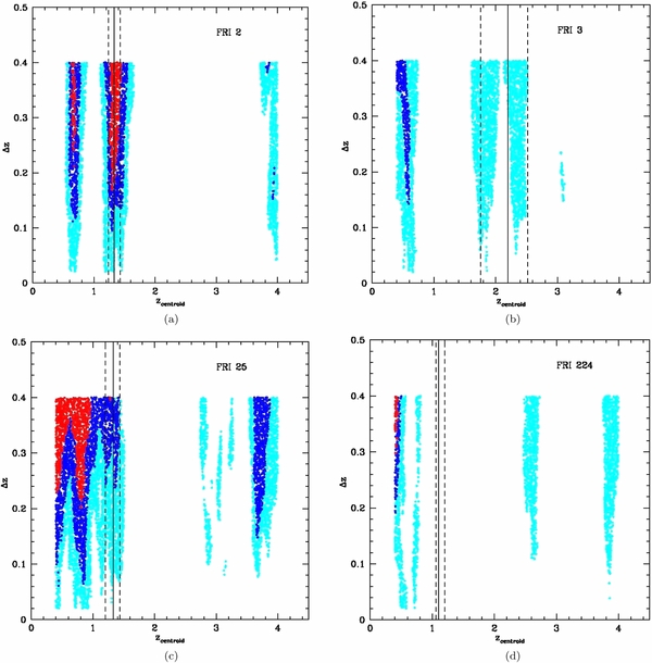
Figure 1. PPM plots for the fields of sources (a) 02, (b) 03, (c) 25, and (d) 224 of the Chiaberge et al. (2009) sample. The abscissa of the vertical solid line is at the redshift of the source. The vertical dashed lines show its uncertainties as given in Baldi et al. (2013). Each point represents the detection significance of the number count excess for a specific choice of the values of the redshift bin Δz (within which we perform the number count) and its centroid zcentroid. The detection significance is estimated as the complementary probability of the null hypothesis (i.e., no clustering) to have more than the observed number of galaxies in the field of the beacon (i.e., the FR I radio galaxy in our case), assuming Poisson statistics and the average number density estimated from the COSMOS field. We plot only the points corresponding to overdensities with a ⩾2σ detection significance. Color code: ⩾2σ (cyan points), ⩾3σ (blue points), and ⩾4σ (red points). A Gaussian filter that eliminates high frequency noisy patterns is applied.
Download figure:
Standard image High-resolution imageOur approach implicitly assumes azimuthal symmetry around the axis oriented at the coordinates of the beacon. Since we extend the tessellation up to ∼6 arcmin (i.e., ∼3 Mpc at z = 1.5) from the coordinates of the beacon, we do not exclude the possibility of detecting non-circularly symmetric systems. (see Postman et al. 1996, for a similar methodology). Furthermore, our method is also flexible enough to find clusters even if the coordinates of the cluster center are known with ∼100 arcsec accuracy (as tested with simulations; see Sections 4.1 and 5.2).
We note that the great majority of low-power radio sources in clusters or groups are found within ∼200 kpc from the core center up to z ≃ 1.3 (Ledlow & Owen 1995; Smolčić et al. 2011). Furthermore, FR Is are typically hosted by undisturbed ellipticals or cD galaxies (Zirbel 1996), which are often associated with the BCGs (von der Linden et al. 2007). Similarly to the FR Is, BCGs are preferentially found within ∼41 kpc from the cluster centers (Zitrin et al. 2012; Semler et al. 2012). Therefore, this suggests that FR Is in cluster environments are preferentially hosted within the central regions of the core, at least at low redshifts. The results presented in the companion paper (see discussion in Section 8.8 of Paper II). for the z ∼ 1–2 cluster candidates associated with the Chiaberge et al. (2009) sample suggest that this is generally true also at higher redshifts. This motivates the peculiar projected space tessellation described in this section and adopted for our cluster search (see the Appendix for further discussion)
In the next section we test the PPM against simulations. We use the COSMOS survey and the photometric redshift catalog of Ilbert et al. (2009). We follow two different approaches: (1) we use two clusters discovered in the COSMOS field at z ∼ 1 and then we shift them to higher redshifts in order to assess the PPM efficiency to detect megaparsec-scale structures at progressively high redshifts. (2) We simulate spherically symmetric clusters of different size and richness, and we locate them at different redshifts (i.e., z = 1.0, 1.5, and 2.0) in the COSMOS field. Then, we apply the PPM and we test if we can detect the simulated clusters.
Note that we do not test our method by adopting mock catalogs derived from N-body numerical simulations to simulate the COSMOS density field shown in previous work for groups in COSMOS up to z ≃ 1 (e.g., George et al. 2011; Jian et al. 2014). This test omission is motivated by the fact that we lack sufficient spectroscopic redshift information. We also have both smaller number count statistics and larger photometric redshift uncertainties, both of which strongly affect these studies at higher redshifts (i.e., z ≳ 1).
3.1. The PPM Theory
In this section we report a sequential list of logical statements that clarify the theory the PPM procedure is based on. We refer to the Appendix for the proofs.
- 1.Since high photometric redshift uncertainties affect any high-z cluster search, the redshifts and projected coordinates of the galaxies are considered separately. The field is tessellated with concentric regions of equal area centered at the projected coordinates of the beacon, i.e., the radio galaxy in our case (see Section A.1).
- 2.Sources with photometric redshifts within the redshift bin Δz centered at the redshift centroid zcentroid are selected. The values of Δz and zcentroid densely span the ranges of our interest (see Section A.2).
- 3.The probability of the null hypothesis (i.e., no clustering) is calculated for each region, given the values of Δz and zcentroid (see Section A.4).
- 4.Starting from the projected coordinates of the beacon, the first consecutive regions for which the null hypothesis is rejected at a level ⩾70% are selected. Then, the regions are merged to form a new one (see Section A.4). This procedure aims at selecting the region in the projected space where the overdensity is present.
- 5.
- 6.Fluctuations of
 on scales δΔz and δzcentroid smaller than the typical statistical photometric redshift uncertainties are not physical and ultimately due to noise. They are locally removed by convolving with a Gaussian filter, i.e., .9 is an effective mean field defined on the space of (zcentroid; Δz); see Section A.5.
 - 7.We apply a variational approach and show that the filter simultaneously suppresses (in linear approximation) the variations of both in the space of (zcentroid; Δz) and in the ensemble of all the possible redshift realizations of the galaxies in the field (see Section A.5). The variations of in the ensemble originated from the fact that photometric redshift uncertainties are neglected when calculating (see Section A.3).
- 8. is a good estimate for (1) the probability that the null hypothesis is rejected, where photometric redshift uncertainties are not neglected and (2) the significance of the number count excess in the field. In fact, the significance of the number count excess is decreased by the filtering procedure to take the additional variance due to the photometric redshift uncertainties into account (see Sections A.3 and A.5).
- 9.We conservatively fix a 2σ wide redshift bin Δz = 0.28 and we apply the peak finding algorithm we developed for our discrete case. Such a procedure belongs to a more general context known as Morse theory (see Section A.6). The algorithm allows us to select the cluster candidates in the field within the redshift range of our interest and, for each overdensity, it provides (1) an estimate for its redshift, (2) an estimate for the cluster core size, and (3) a rough estimate for the cluster richness (see Section A.7).
- 10.The association of the cluster candidates detected in the field with the beacon (i.e., in our case the radio galaxy) is performed by using the cluster redshift estimate and the redshift of the radio galaxy, as well as the corresponding uncertainties (see Section A.8).
- 11.A generalization of the method to other data sets and surveys is provided in Section A.10.


4. CLUSTERS AT z ≃ 1 SHIFTED TO HIGHER REDSHIFTS
In this section we test the effectiveness of the PPM in detecting overdensities as a function of redshift. We consider the z ∼ 1 cluster candidates with ID numbers 62 and 126 (hereafter F062 and F126, respectively) in the Finoguenov et al. (2007, hereinafter FGH07) group COSMOS catalog, selected by using XMM-Newton observations (Hasinger et al. 2007).
F062 is in the field of the source COSMOS-FRI 01. This source is part of the C09 sample and it is found in rich megaparsec-scale environment by the PPM (see Paper II for further discussion). The offset between the X-ray centroid of F062 (estimated in FGH07) and the projected coordinates of COSMOS-FRI 01 is about ∼10 arcsec. This corresponds to 78 kpc at the spectroscopic redshift of the radio galaxy, i.e., zspec = 0.88 (Lilly et al. 2007; Trump et al. 2007). The redshift of F126 as estimated in FGH07 is z = 1.0. FGH07 also estimated masses M500 = (5.65 ± 0.37) × 1013 M☉ and (6.87 ± 0.69) × 1013 M☉ for F062 and F126, respectively.10
In Figure 2 we plot the RGB images of F062 (left panel) and F126 (right panel) centered at the X-ray coordinates of the clusters, as in FGH07. We plot as green circles the locations of the galaxies in the Ilbert et al. (2009) catalog with photometric redshifts within a Δz = 0.2 long redshift bin centered at the redshift of the cluster. Concerning F062, we show as a yellow circle the location of COSMOS-FRI 01. The images are obtained using Spitzer 3.6 μm, and Subaru r- and V-band images for the R, G, and B channels, respectively. As clear from visual inspection, both F062 and F126 exhibit a clear segregation of red objects within their megaparsec-scale core. Note that the brightest cluster member of F126 is associated with a radio source that is below the flux threshold of the C09 catalog. The two groups considered here also have comparable core sizes, X-ray fluxes, luminosities, and temperatures (see Table 1 in FGH07 for further details). They have similar X-ray properties, but F126 seems significantly richer than F062 (see Figure 2). Hence, we prefer to consider both of them, instead of only one. This is in order to make our conclusions more robust. In fact, if we adopted one single cluster candidate, our simulations might be biased by the specific properties of that overdensity and our results might not be valid in a more general sense. In the following we outline the different tests we perform. In Section 4.1 we will describe the results in detail.
- 1.First, we apply the PPM and we test if it detects F062 and F126 (at their actual redshift).
- 2.We apply the PPM using increasing offsets between coordinates of the center of the PPM tessellation and the X-ray coordinates of the cluster center. This is done to estimate the required accuracy in the projected coordinates of the cluster center in order to detect cluster candidates with the PPM.
- 3.We shift both F062 and F126 to higher redshifts and we test whether the PPM is able to detect them. The procedure is quite complex and we describe it in the following. We select the fiducial cluster members by adopting a color (I − K)AB selection criterion to identify the redder sources. A cluster membership is required since we want to shift the cluster members to increasing redshifts. The cluster members are selected within a redshift bin centered at the redshift of the cluster candidate and within a projected area centered at the X-ray cluster coordinates. Both the redshift bin and the projected area are selected according to the PPM, as we will discuss in detail. A color selection is preferred to a cluster membership assigned on the basis of the photometric redshift information. Our choice is motivated by the fact that we select galaxies that are in the field and at the redshift of F062 and F126, until the mean COSMOS density is reached. A selection based on the photometric redshift information (e.g., Papovich et al. 2010) might be biased toward selecting cluster galaxies as well as field galaxies. This would imply an overestimation of the number of the cluster members as well as of the number count excess associated with F062 and F126. Conversely, our color criterion avoids it, since we select galaxies starting from the reddest ones, which are most likely the elliptical galaxies of the cluster.We subtract the cluster members from the fields of F062 and F126. We apply the PPM to see if any residual structure is detected and if the cluster membership has been correctly assigned. Some of the cluster members may not have been identified. If this is the case, the PPM might still detect an overdensity in the field, once the cluster members are subtracted. However, the opposite case in which too many sources are selected as cluster members is not tested with this approach. This is because the PPM is not used to detect the presence of underdense regions.We add the fiducial cluster members to the fields of two sources of the C09 sample, namely COSMOS-FRI 70 and COSMOS-FRI 66, where no overdensity is detected by the PPM in the redshift range z ∼ 1–2 of our interest (see also Paper II). This is done applying a rigid rotation to the projected coordinates of the selected cluster members. Two fields are used because weak overdensities not detected by the PPM procedure might be present in the redshift range of our interest. Therefore, the clusters would be more easily detected if their members are shifted to the redshifts of these non-detected overdensities. This might imply that the cluster detection significance is overestimated. The choice of the two fields reduces the possibility that this bias occurs. Then we apply the PPM in the new field to test if megaparsec-scale overdensities is still detected.We shift the fiducial cluster members to zc, sim = 1.5, 2.0. We firstly estimate the AB I-band magnitude Isim that each of the cluster member would have if located at higher redshift zc, sim. Then we reject all of the cluster members with Isim ⩾ 25. This is the same selection criterion applied in Ilbert et al. (2009) in estimating the photometric redshifts. This is done to simulate the COSMOS sensitivity and to properly reject the faintest galaxies that would not be detected when shifted to a redshift higher than their own.We assign a photometric redshift to each of the cluster members selected with the previous procedure, according to a Gaussian probability distribution. The average is set equal to the redshift of the simulated cluster zc, sim. We adopt a variance equal to the square of the typical statistical 1σ accuracy σz(zc, sim) = 0.054(1 + zc, sim) of the photometric redshifts around zc, sim for sources with i+ ∼ 24 and redshifts within 1.5 < z < 3 (see Table 3 of Ilbert et al. 2009), typical of the cluster galaxies we consider. This is done in order to assign properly a photometric redshift to each of the cluster members once they are shifted to a redshift higher than the true redshift of the cluster.We finally apply the PPM to see if the clusters are still detected by the PPM at z = 1.5 and 2.0.
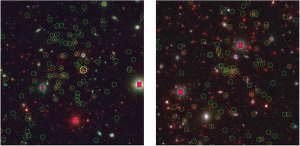
Figure 2. RGB images of F062 (left) and F126 (right) centered at the X-ray coordinates of the clusters, as in FGH07. The images are obtained using Spitzer 3.6 μm, and Subaru r+- and V-band images for the R, G, and B channels, respectively. Green circles indicate objects with 0.78 < zphot < 0.98 (left) and 0.9 < zphot < 1.1 (right). The yellow circle in the left panel shows the location of COSMOS-FRI01. The projected sizes of the fields are 180'' × 180''. North is up.
Download figure:
Standard image High-resolution image4.1. Results
- 1.In Figure 3 we show the PPM plots (as in Figure 1, see Section 3) for F062 (left) and F126 (right). We adopt the following color code: ⩾2σ, ⩾3σ, and ⩾4σ points are plotted in cyan, blue, and red, respectively. The abscissa of the vertical solid line indicates the redshift of the cluster candidate.In Table 1 we report the PPM results for F062 and F126 (top part). We also report the PPM results of our simulations, when these two clusters are added to the fields of COSMOS-FRI 66 and COSMOS-FRI 70 of the Chiaberge et al. (2009) sample (middle part). In the bottom part of the table, we report the PPM results where the clusters are shifted to z = 1.5. In the first four columns we list the cluster ID number (i.e., F062, F126), the cluster redshift, the cluster redshift as estimated by the PPM, and the cluster detection significance. In the fifth column we report the distance rmax from the location of the radio galaxy in the projected space at which the overdensity formally ends. For the above quantity, the average, the rms dispersion around the average, and the median value (inside parentheses) in units of arcsec are reported, as estimated by the PPM procedure. The rms dispersion and the median value are not reported where the former is null, i.e., where the estimated rmax is maximally stable with respect to zcentroid, i.e., where the rms dispersion is null. In the sixth column we report the field to which the cluster is added; 66 and 70 denote that the cluster members are added to the fields of COSMOS FR I 66 and COSMOS FR I 70, respectively. The symbol "—" denotes that the PPM is applied to the fields of F062 and F126, where the cluster members are not subtracted.Concerning the PPM results for F062 and F126 (top part), they are detected with significance levels of 3.8σ and 4.3σ, respectively. The estimated redshifts are z = 0.86 and z = 0.96, respectively. In addition to the cluster candidate at z ∼ 1, the PPM detects another 2.7σ overdensity in the field of F126 at z = 0.64. This is a clear example of a projection effect.Note that our redshift estimates fully agree with the actual redshifts of the two cluster candidates (i.e., z = 0.88 and z = 1.0 for F062 and F126, respectively) and that the PPM effectively finds systems whose masses are compatible to those of rich groups and, therefore, they are even below the typical cluster mass cutoff ∼1 × 10¹⁴ M☉, as is the case with F062 and F126. Hereinafter we do not estimate the redshift uncertainties following the PPM procedure prescription. This is mainly because we know the redshift of the cluster in our simulations. Therefore, we can directly compare our estimates with the original cluster redshifts to derive the statistical uncertainties. Conversely, in Paper II we estimate redshift uncertainties (following the procedure described above) for the overdensities we find within the C09 sample.
- 2.We then apply the PPM using increasing offsets θoff between the cluster center of the PPM tessellation and the actual center as measured from the X-ray emission. This is done to find the required accuracy in the coordinates of the cluster center in order to detect megaparsec-scale overdensities with the PPM. We keep the right ascension of the center of the PPM tessellation fixed and we change its declination from θoff =10 up to 500 arcsec.We find that F062 and F126 are detected up to θoff = 150 and 500 arcsec, respectively. The clusters are detected with a fairly constant significance (between ∼3.2–3.8σ and ∼3.7–4.8σ for F062 and F126, respectively). However, a mild trend of decreasing significance for increasing offsets is observed. F062 is detected with significances of 3.8σ, 3.2σ, and 3.2σ at θoff = 0, 75, and 150 arcsec, respectively. In fact, F126 is detected with significances of 4.3σ, 3.9σ, 3.7σ, and 3.7σ at θoff = 0, 100, 300, and 500 arcsec, respectively.A clear trend between rmax and θoff is observed for F062. The estimated size increases up to rmax ≃ 150 arcsec for θoff = 125 arcsec. While the estimated size for θoff = 0 arcsec is rmax = 72.6 ± 5.1 arcsec. Conversely, no trend is observed for F126.These results suggest that the PPM is effective to detect megaparsec-scale overdensities even if the projected coordinates of the cluster center are known with an accuracy of only ∼100 arcsec. This implies that the PPM can be efficiently applied even if the cluster center coordinates are not accurately known.
- 3.We want to shift these two groups to redshifts higher than z ∼ 1, thus we select the fiducial cluster members of both F062 and F126. We select those sources that fall within circular regions of radius 70.7 and 165.8 arcsec centered at the coordinates of the cluster center, for F062 and F126, respectively. These are the regions in the projected space within which the clusters are detected by the PPM.We conservatively select sources with photometric redshifts within a redshift slice Δz = 4σz(zc) centered around the redshift zc of the cluster, where σz(zc) = 0.054(1 + zc) is the 1σ statistical photometric redshift uncertainty of faint galaxies with i+ ∼ 24 and 1.5 < z < 3 sources (see Table 3 of Ilbert et al. 2009), typical of the cluster galaxies we consider. The redshift slice considered here is bigger than that adopted throughout the PPM procedure (i.e., Δz = 0.28) to make sure that the large majority of the sources at the redshift of the cluster are included in the bin, even if the accuracy of their photometric redshifts is poor. This is not a cluster membership assignment. In fact, the cluster members will be selected among these sources by using an (I − K)AB color criterion, as we will describe in the following.11Since red and passively evolving galaxies constitute the majority among the cluster core galaxies at z ∼ 1, we also adopt a color selection criterion to define the fiducial cluster members. We sort the selected galaxies according to their (I − K)AB color, from redder to bluer. This specific color criterion has been chosen because the rest frame ∼4000 Å absorption feature typical of the spectra of early type galaxies falls just between the K and I bands at redshift z ∼ 1.The cluster members are then removed from the field starting from the reddest source until the average COSMOS number density within the selected 4σz bin is reached.According to the outlined procedure we select as cluster members 57 and 249 galaxies down to (I − K)AB = 1.12 and 1.30 magnitudes for F062 and F126, respectively. As expected, these cluster members are faint, since their I-band magnitudes are between I ∼ 21.9–25.3 and I ∼ 21.1–25.7 for F062 and F126, respectively.We want to make sure that the cluster membership is not biased toward preferentially selecting sources that are located in certain regions in the projected space around the cluster center. In order to do this we verify whether the differential radial number counts are consistent with a constant—no clustering—once the cluster members are removed from the field.In Figure 4 we plot the differential number counts of the sources in the fields of F062 (left panel) and F126 (right panel), as a function of the distance from the projected cluster center coordinates. Sources are counted within the 4σz redshift slice adopted throughout the cluster membership procedure and within regions of equal areas (i.e., 2.18 arcmin2), analogously to what was done for the PPM. The areas are chosen to be equal among each other in order to have a constant mean field density per region.The galaxy number counts along with the corresponding 1σ Poisson uncertainties for the error are plotted as blue symbols. Number counts, once the cluster members are subtracted from the fields of both F062 and F126, are plotted as black points, along with the 1σ uncertainties estimated according to the Skellam distribution.12 The uncertainty in the radial coordinate corresponds to the half-width of each region.The vertical red dashed lines show the radial interval within which the cluster members are selected. By construction, according to the cluster membership procedure, black and blue points coincide outside of this interval. The horizontal line shows the mean COSMOS number counts of ∼30 galaxies associated with a 2.18 arcmin2 area around which the black points are scattered.The radial profiles of both F062 and F126 clearly show that the number count excess (blue points) is limited within the projected area defined within the vertical dashed lines. Furthermore, once the cluster members are subtracted, such a number count excess disappears. In fact, the values associated with the black points are consistent with the mean COSMOS number density within the reported 1σ uncertainties.In Figure 5 we report the PPM plots of the fields of F062 and F126, where the cluster members are subtracted. The adopted color code is analogous to that of Figure 3. We apply the PPM and we verify that neither F062 nor F126 are now detected. In fact, as is clear from visual inspection, the high significance pattern at the redshift of the cluster completely disappears in the case of F062, while a residual ≳ 2σ feature is still present in the case of F126 at its redshift. According to the PPM procedure, such a feature is interpreted as noise because it is not enough extended to be detected as overdensity, i.e., it is less than δzcentroid = 0.1 long on the redshift axis zcentroid at fixed Δz = 0.28.The other megaparsec-scale overdensity that was previously detected by the PPM in the field of F126 at z = 0.64 with a significance of 2.7σ is still detected with similar significance (2.6σ) and redshift (z = 0.61). This confirms that the specific cluster membership assigned here combined with the PPM is efficient at removing the degeneracy resulting from the projection effect.As explained above, for our simulations we perform the cluster membership by selecting fiducial cluster members within a circular region centered at the X-ray coordinates of F062 and F126. The radius of the region corresponds to the projected size of the cluster, as estimated by the PPM. In the following we reconsider our estimates by using the PPM plots and we compare the fiducial sizes estimated with the PPM with those obtained by previous work.In Figure 6 we report the PPM plots for F062 (left panel) and F126 (right panel), where only the points corresponding to ⩾3σ overdensities are plotted. This is because the two clusters are detected with significance higher than 3σ. Since we are interested in the cluster size, we plot the cluster size (rmax ) associated with each point in the plot, as estimated by the PPM for specific zcentroid and Δz. We refer to the legend in Figure 6 for the specific color code adopted. As clear from visual inspection of the plots, the values of rmax are stable with respect to the Δz parameter.By averaging among the values associated with the points at Δz ≃ 0.28 that define the overdensities, we estimate the sizes rmax = 72.6 ± 5.1 arcsec and rmax = 181.3 ± 33.4 arcsec for F062 and F126, respectively, according to the PPM procedure. Here we report the average value and the rms dispersion around the average. The cluster sizes 70.7 arcsec and 165.8 arcsec that are assumed when performing the cluster membership correspond to the median values of rmax for F062 and F126, respectively.Based on the X-ray surface brightness, FGH07 estimated a core size r500 = 48 arcsec for both F062 and F126. By assuming spherical symmetry and a β-model density profile for the cluster matter distribution (Cavaliere & Fusco-Fermiano 1978) we estimate r200 = 76 arcsec for both F062 and F126.13George et al. (2011) estimated core sizes of r200 = 73 arcsec and 81 arcsec and core masses M200 = 5.25 × 10¹³ M☉ and 8.32 × 10¹³ M☉, for F062 and F126,14 respectively, on the basis of the mass versus X-ray luminosity relation given in Leauthaud et al. (2010). Using spectroscopic redshift information, Knobel et al. (2012) estimated a size of 659 kpc (i.e., ∼84 arcsec at the redshift of the cluster) for F062.We find that our size estimates are in good agreement with those reported by previous work. However, for F126 our estimate is higher than previous work.Since we want to shift the cluster members of both F062 and F126 to higher redshifts we select two fields where no overdensity is detected with the PPM in the redshift range z ∼ 1–2. We prefer to shift the cluster members of both F062 and F126 into other fields because we want to make sure than no overdensity is detected by the PPM in the redshift range z ∼ 1–2 for the considered field. We note in fact that this is not the case of F062, i.e., a 2.4σ overdensity is detected at z = 2.00. Furthermore, the choice of the same field for both F062 and F126 allows us to directly compare the results we obtain with the PPM for the two clusters, once the cluster members are added to such a field.In Figure 7 we report the PPM plots for the fields of COSMOS-FRI 66 (left panel) and COSMOS-FRI 70 (right panel). As clear for visual inspection of the plots, no high significance pattern is detected in these plots within the redshift range z ∼ 1–2. A weak 2σ overdensity is detected by the PPM at redshift z = 1.60 in the field of COSMOS-FRI 66. However, such a feature is not detected if a slightly different redshift bin (i.e., Δz = 0.24) is adopted throughout the PPM procedure. All of the other isolated ≳ 2σ patterns clearly visible in the plots are interpreted as noise. This is because either they are not located around the y-axis value Δz = 0.28 that is relevant for the overdensity detection or they are not extended enough to be detected as an overdensity (i.e., they are less than δzcentroid = 0.1 long on the redshift axis zcentroid at fixed Δz = 0.28), according to the PPM procedure.Since no clear overdensity is detected in the fields of COSMOS-FRI 66 and COSMOS-FRI 70 we use them as empty control fields (ECFs). Note that we cannot exclude the presence of underdense or dense regions that are not detected by the PPM but are still present in these two ECFs at the redshifts of our interest.If a cluster is superimposed on an underdense region, the PPM might underestimate the detection significance or it might detect no overdensity. Conversely, if the cluster is added to an overdense region, the PPM tends to overestimate the overdensity significance. The reason to choose two ECFs instead of one is to see whether these two scenarios occur. In particular, we will compare our results obtained from each ECF separately to look for a possible mismatch.We add to each ECF the fiducial cluster members of F062 and F126, separately, and we apply the PPM at the coordinates of COSMOS-FRI 66 and COSMOS-FRI 70.15 In Figure 8 we report the resulting PPM plots, where the clusters F062 (left panel) and F126 (right panel) are in the field of COSMOS-FRI 70. As is clear from visual inspection of the plots, both F062 and F126 are still detected at their true redshift with significances between ∼3–4σ. In Table 1 (middle part) we report the PPM results of our simulations. The estimated redshifts for F062 and F126 are z = 0.86 and z = 1.0, respectively, where the cluster members are added to the fields of COSMOS-FRI 70. Therefore, the estimated redshifts fully agree with those of the clusters. The estimated sizes of F062 and F126 are rmax = 74.3 ± 6.7 arcsec and rmax = 92.0 ± 10.0 arcsec, respectively, where the cluster members are added to the field of COSMOS-FRI 70. These size estimates agree, independently of the ECF adopted (within the errors), with those previously obtained where the cluster members are not subtracted from their own fields (see Table 1, top). These results suggest that the cluster properties estimated by the PPM are not affected by the applied cluster membership and by the fact that the cluster members are added to a field different from that original of the cluster.In order to shift the cluster members of both F062 and F126 to higher redshifts (i.e., zc = 1.5 and 2.0) we need to address the problem of the detection limit. The COSMOS number density drops off rapidly with increasing redshift. In fact, the number density per unit redshift is, on average, dn/dz/dΩ ≃ 25, 10, and 3 arcmin−2 at redshifts z ∼1, 1.5, and 2.0, respectively (see Ilbert et al. 2009). Therefore we expect some of the selected cluster members would not be detected if they were located at higher redshifts since their flux would be lower than the survey threshold.In order to address this problem we estimate the I-band magnitude each cluster member would have if it were located at a higher redshift. Then we reject all the sources with I ⩾ 25, that is the magnitude cut applied to the Ilbert et al. (2009) catalog.We assume that each cluster member is located at the redshift of the clusters F062 and F126, i.e., zc = 0.88 and 1.0, respectively. Then, we estimate the simulated I-band magnitude each cluster member would have if shifted to zc, sim = 1.5 and 2.0. Practically, we perform the K-correction by using the spectral energy distribution (SED) of each object, i.e., we linearly interpolate the flux measurements reported in the I09 catalog, and we correct the apparent magnitude for the luminosity distance.Then, as outlined above, we reject all the members for which IAB ⩾ 25. This procedure reduces the number of the cluster members from 57 to 9 sources (zc, sim = 1.5) and to 1 source (zc, sim = 2.0) in the case of F062 and from 249 to 58 (zc, sim = 1.5) and 9 galaxies (zc, sim = 2.0) for F126. We note that the magnitude cut (I < 25) is applied in the Ilbert et al. (2009) to the I(auto) magnitude, that corresponds to the Subaru i+ band magnitude obtained with SExtractor (Bertin & Arnouts 1996). Therefore, the I(auto) magnitudes should be considered instead of the I (Subaru or CFHT) magnitudes. However, we prefer to adopt the I magnitude instead of the I(auto) magnitude because the latter is automatically estimated by SExtractor and, therefore, the former is more reliable for our simulations. However, we verify that the I(auto) magnitudes of the selected cluster members are, on average, only 0.3 ± 0.4 and 0.3 ± 0.2 lower than the corresponding I magnitudes for F062 and F126, respectively. The reported uncertainty is the rms dispersion around the average. Therefore, the I magnitudes are consistent within ∼1σ with the I(auto) magnitudes for the selected cluster members. This suggests that the results of our simulations would not change if we chose the I(auto) instead of the I magnitudes.In the following we will address the problem of assigning coordinates to the cluster members of both F062 and F126 when they are located at zc, sim ⩾ 1.5. The K-correction applied here ignores any contribution from possible evolution.
- 4.Having addressed the problem of cluster membership, we assign fiducial coordinates to each of the cluster members, when the overdensity is shifted to a higher redshift. We assume that the coordinates in the projected space of each galaxy remain unchanged when the overdensity is shifted to higher redshift. Therefore, projection effects and the peculiar motions of the galaxies are neglected. This approximation is good enough because a high accuracy of the projected coordinates of the cluster members is not required in order to apply the PPM. In fact, each area of the PPM tessellation has a projected size of a few ∼100 kpc. Such a size is much larger than the projected positional uncertainty resulting from our approximation.Concerning the galaxy redshifts, we assume that all the selected members are at the same distance to the observer, corresponding to redshift zc, sim = 1.5, 2.0, equal to that of the simulated cluster. Then, we assign to each cluster member a photometric redshift accordingly to a Gaussian probability distribution centered at the redshift of the cluster zc, sim and a standard deviation σc, sim = 0.054(1 + zc, sim).This value corresponds to the 1σ statistical photometric redshift uncertainty of i+ ∼ 24 and 1.5 < z < 3 sources (see Table 3 of Ilbert et al. 2009), typical of the cluster galaxies we consider.
- 5.We shift both F062 and F126 to higher redshift, i.e., zc, sim = 1.5, where the cluster members are added to the fields of COSMOS-FRI 66 and COSMOS-FRI 70, separately. In Figure 9 we report the corresponding PPM plots for both F062 (left panel) and F126 (right panel). The vertical solid line is located at the redshift of the overdensity. As clear from visual inspection of the PPM plots, both F062 and F126 are still detected if they are located at zc, sim = 1.5. In Table 1 (bottom part) we report the PPM results for these simulations. F062 and F126 are detected with 2.9σ and 2.5σ significance levels; the estimated redshifts are z = 1.56 and z = 1.59, respectively, if the cluster members are added to the field of COSMOS-FRI 70. This suggests that the PPM is effective in finding high-redshift groups at z ≃ 1.5, albeit with lower significance than at z ∼ 1 (i.e., ∼2.5–3σ). The estimated sizes for both F062 and F126 are consistent, within the reported errors, with those previously obtained for these two clusters at their true redshift (see Table 1, top part) The results are quite independent of the ECF considered. Neither F062 nor F126 is detected at zc, sim = 2.0.

Figure 3. PPM plots for the cluster candidates F062 (left), F126 (right), as given in FGH07. Overdensities: ⩾2σ (cyan points), ⩾3σ (blue points), ⩾4σ (red points). The vertical solid lines indicate the redshift of the cluster candidate.
Download figure:
Standard image High-resolution image
Figure 4. Blue points: differential number counts of the sources in the fields of F062 (left panel) and F126 (right panel), as a function of the distance from the cluster center coordinates. Sources are counted within a Δz = 4σz redshift bin centered at the redshift of the cluster (i.e., Δz = 0.406 and 0.432 for F062 and F126, respectively). Black points: differential number counts, as for blue points, where the cluster members are subtracted from the field of the cluster. Number count 1σ uncertainties are plotted along the y-axis. The uncertainty in the radial coordinate is the half-width of each region within which the number counts are performed. Vertical dashed lines show the region where the cluster members are selected. The horizontal solid red line shows the mean COSMOS number count per area.
Download figure:
Standard image High-resolution image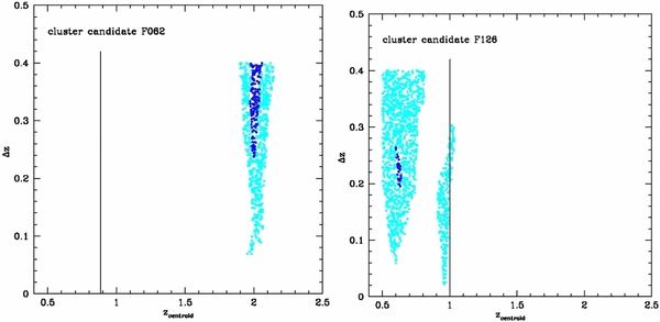
Figure 5. PPM plots where the clusters F062 (left) and F126 (right), in the FGH07 catalog, are subtracted. Overdensities: ⩾2σ (cyan points), ⩾3σ (blue points), and ⩾4σ (red points). The vertical solid line indicates the redshift of the cluster candidate. Note that no ⩾4σ overdensity is present in the plots.
Download figure:
Standard image High-resolution image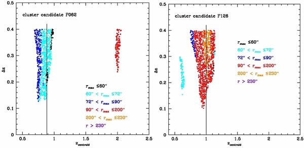
Figure 6. PPM plots for F062 (left) and F126 (right). We plot only those points that correspond to ⩾3σ overdensities for a specific choice of the redshift bin Δz and its centroid zcentroid. Different colors correspond to different values of the cluster size rmax associated with each point and estimated with the PPM. See the legend in the plots for further information about the color code adopted.
Download figure:
Standard image High-resolution image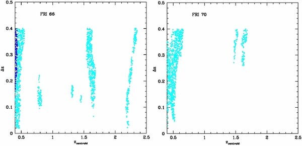
Figure 7. PPM plots for the fields of COSMOS-FRI66 (left) and COSMOS-FRI70 (right) in the Chiaberge et al. (2009) sample. Overdensities: ⩾2σ (cyan points), ⩾3σ (blue points), ⩾4σ (red points). Note that no ⩾4σ overdensity is present in the plots.
Download figure:
Standard image High-resolution image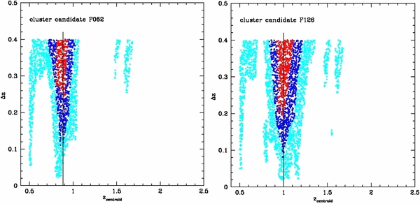
Figure 8. PPM plots of F062 (left) and F126 (right), where their cluster members are added to the field of COSMOS-FRI70. The vertical solid line in each panel is located at the redshift of the cluster. Overdensities: ⩾2σ (cyan points), ⩾3σ (blue points), and ⩾4σ (red points).
Download figure:
Standard image High-resolution image
Figure 9. PPM plots for the F062 (left panel) and F126 (right panel), shifted at zc, sim = 1.5 and located in the field of COSMOS-FRI70. The abscissa of the vertical solid line is at the redshift of the overdensity (zc, sim = 1.5). We plot only the points corresponding to detected overdensities for different values of Δz and zcentroid. Color code: ⩾2σ (cyan points), ⩾3σ (blue points), and ⩾4σ (red points). The Gaussian filter that eliminates high frequency noisy patterns is applied. Note that no ⩾4σ overdensity is present in the plots.
Download figure:
Standard image High-resolution imageTable 1. PPM Results
| F062 and F126 | |||||
|---|---|---|---|---|---|
| ID | zcluster | zPPM | Significance | rmax (arcsec) | Field |
| F062 | 0.88 | 0.86 | 3.8σ | 72.6 ± 5.1 (70.7) | — |
| F126 | 1.00 | 0.96 | 4.3σ | 181.3 ± 33.4 (165.8) | — |
| F062 and F126 added to the ECFs | |||||
| ID | zcluster | zPPM | Significance | rmax (arcsec) | Field |
| F062 | 0.88 | 0.86 | 3.5σ | 71.6 ± 3.6 (70.7) | 66 |
| F062 | 0.88 | 0.86 | 4.0σ | 74.3 ± 6.7 (70.7) | 70 |
| F126 | 1.00 | 0.94 | 4.9σ | 109.9 ± 6.1 (111.8) | 66 |
| F126 | 1.00 | 1.00 | 4.1σ | 92.0 ± 10.0 (86.6) | 70 |
| F062 and F126 added to the ECFs and shifted to higher redshift | |||||
| ID | zcluster | zPPM | Significance | rmax (arcsec) | Field |
| F062 | 1.50 | 1.61 | 2.6σ | 50.0 —— | 66 |
| F062 | 1.50 | 1.56 | 2.9σ | 50.0 —— | 70 |
| F126 | 1.50 | 1.51 | 3.1σ | 111.3 ± 2.4 (111.8) | 66 |
| F126 | 1.50 | 1.59 | 2.5σ | 85.4 ± 4.2 (86.6) | 70 |
Notes. PPM results for F062 and F126 where the cluster members are not removed (top part). PPM results where the cluster members are added to the ECFs (middle part) and where they are also shifted to z = 1.5 (bottom part). Column description: (1) cluster ID number; (2) cluster redshift; (3) cluster redshift estimated with the PPM; (4) significance of the overdensity estimated by the PPM in terms of σ; (5) average maximum radius (arcsec) of the overdensity along with the rms dispersion around the average (both estimated with the PPM). The median value (arcsec) is written between the parenthesis. The rms dispersion and the median value are not reported in those cases where the rms dispersion is null; (6) field to which the cluster is added; 66 and 70 denote that the cluster members are added to the fields of COSMOS-FRI 66 and COSMOS-FRI 70, respectively. The symbol "—" denotes that the PPM is applied to the fields of F062 and F126, where the cluster members are not subtracted.
Download table as: ASCIITypeset image
5. SIMULATED CLUSTERS
We now perform another set of simulations, by creating simulated clusters with different richness and size. Then, we apply the PPM to test if they are detected at different redshifts.
We consider as cluster members Nc sources uniformly distributed within a sphere of comoving radius Rc centered at the redshift zc.
We consider both ECFs used in Section 4 and four additional ECFs (denoted by ECF 3, 4, 5, and 6) where no overdensity is detected by the PPM within the redshift range z ∼ 1–2. We increase the number of ECFs with respect to our previous analysis because the ECFs might host some overdensities that are just slightly below the 2σ PPM detection threshold, but they might be detected once other galaxies are added to the same field. The effect of overdensities and underdensities in the location of our simulated clusters should be marginalized with the increased number of random fields. In Figure 10 we report the PPM plots for the four additional ECFs. Concerning the cluster sizes, in this section we only refer to comoving sizes, unless otherwise specified.
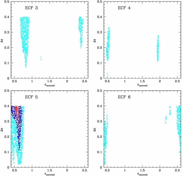
Figure 10. PPM plots for the four additional ECFs. Overdensities: ⩾2σ (cyan points), ⩾3σ (blue points), and ⩾4σ (red points).
Download figure:
Standard image High-resolution imageWe choose the following parameters: Nc = 10, 30, 60, 100, 150, and 200; zc = 1.0, 1.5, and 2.0; Rc = 1.0, 2.0, and 3.0 Mpc. This results in 54 simulated clusters obtained by considering all the possible combinations of the values of Nc, zc, and Rc. In particular, the redshifts are chosen in the range of our interest, while the adopted comoving sizes and the considered values for the richness are typical of clusters and groups we expect to find in the COSMOS survey adopting our method.
In fact, in Paper II we estimate cluster core sizes for the z ∼ 1–2 cluster candidates found in the fields of the Chiaberge et al. (2009) sample. Average physical and comoving core sizes rmax = (772 ± 213) kpc and rmax = (1762 ± 602) kpc are obtained, respectively. The average is performed using all the cluster candidates, and the reported uncertainty is the 1σ rms dispersion around the average.
As discussed in Paper II, the estimated number of the fiducial cluster members varies with the cluster detection significance from ∼10 for our cluster candidates at the highest redshifts (z ∼ 2) to more than ∼200 for our z ∼ 1 clusters candidates.
Note that clusters of galaxies usually include up to thousands of galaxies. Here we adopt smaller values for Nc because the Ilbert et al. (2009) catalog lacks faint I > 25 galaxies that still constitute a significant fraction of the cluster galaxies at redshifts z ≳ 1 (Rudnick et al. 2012).
As discussed in Paper II, mass estimates are found in the literature for some of our cluster candidates at redshift z ∼ 1. In particular, FGH07 estimated a cluster mass M500 = 5.65 × 10¹³ M☉ for the rich group associated with source 01, for which the PPM selects ∼100 cluster members within a circle of rmax = 70.7 arcsec radius and a redshift bin Δz = 0.28 centered at the spectroscopic redshift z = 0.88 of the cluster. Knobel et al. (2009, 2012) reported masses within M ∼ 1.4–2.2 × 10¹³ M☉ for the cluster candidates in the fields of sources 16, 18, and 20 for which ∼100, ∼200, and ∼100 fiducial cluster members are selected by the PPM, respectively. Source 16 has a spectroscopic redshift z = 0.97, while the photometric redshifts of sources 18 and 20 are z = 0.92 and z = 0.88, respectively. As pointed out in Section 4.1, such mass estimates and cluster detections further suggest that PPM effectively finds systems whose masses are compatible with those of rich groups. Therefore, the PPM is able to detect structures whose mass is even below the typical cluster mass cutoff ∼1 × 10¹⁴ M☉.
For a given simulated cluster we change the exact redshift of each of the Nc members to account for the observational uncertainties. Conversely, we do not change their projected coordinates of the cluster members because the angular positional uncertainties are negligible with respect to the photometric redshift uncertainties (Ilbert et al. 2009). For the same reason, we also neglect the galaxy peculiar velocities and, therefore, all of the cluster members are assumed to be at the same redshift zc. We assign to each of the Nc sources a photometric redshift drawn from a Gaussian probability distribution centered at the mean zc and whose standard deviation is σc = 0.054(1 + zc). This is the 1σ statistical photometric redshift uncertainty of i+ ∼ 24 and 1.5 < z < 3 sources (see Table 3 of Ilbert et al. 2009), typical of the cluster galaxies we consider, consistent with what has been done throughout this work (see, e.g., Section 4).
We consider the case where (1) the equatorial coordinates at which we choose to center the tessellation of the PPM, (2) the equatorial coordinates of the adopted ECF and (3) the equatorial coordinates of the center of the spherically symmetric simulated cluster all coincide. In particular, for our simulations we keep (1) the equatorial coordinates at which we choose to center the tessellation of the PPM and (2) the equatorial coordinates of the adopted ECF unchanged, i.e., (1) and (2) will always coincide. The ECFs are in fact chosen because the PPM does not detect any overdensity in these fields at the redshift range (z ∼ 1–2) of our interest. Conversely, some overdensities might be present at a certain offset from the equatorial coordinates of the adopted ECF. In this case the PPM might detect these overdensities if the equatorial coordinates at which we choose to center the PPM tessellation do not coincide with those of the center of the adopted ECF.
However, in order to test the efficiency of the PPM to detect clusters if the cluster center coordinates are not accurately known, in Section 5.2 we will offset (by an angle θ) the input PPM coordinates with respect to the center of the spherically symmetric simulated cluster.
5.1. General Results and Trends
In Table 2 we summarize the results for all 54 simulated clusters. Each entry of the table shows the fraction of ECFs in which the cluster with specific values of Nc, Rc, and zc is detected. For example, the fraction 4/6 means that the cluster is detected in four out of the six ECFs.
Table 2. Simulated Cluster Detections (Null Offset)
| Rc | Nc = 10 | Nc = 30 | Nc = 60 | Nc = 100 | Nc ⩾ 150 | ||||||||||
|---|---|---|---|---|---|---|---|---|---|---|---|---|---|---|---|
| (Mpc) | zc = 1 | 1.5 | 2 | 1 | 1.5 | 2 | 1 | 1.5 | 2 | 1 | 1.5 | 2 | 1 | 1.5 | 2 |
| 1.0 | 0/6 | 4/6 | 5/6 | 6/6 | 6/6 | 6/6 | 6/6 | 6/6 | 6/6 | 6/6 | 6/6 | 6/6 | 6/6 | 6/6 | 6/6 |
| 2.0 | 0/6 | 3/6 | 3/6 | 1/6 | 5/6 | 6/6 | 5/6 | 6/6 | 6/6 | 6/6 | 6/6 | 6/6 | 6/6 | 6/6 | 6/6 |
| 3.0 | 0/6 | 2/6 | 3/6 | 0/6 | 4/6 | 6/6 | 0/6 | 6/6 | 6/6 | 4/6 | 6/6 | 6/6 | 6/6 | 6/6 | 6/6 |
Notes. Detection results for the simulated clusters with different input richness (Nc), redshift (zc), and size (Rc), in the case where (1) the equatorial coordinates at which we choose to center the tessellation of the PPM, (2) the equatorial coordinates of the adopted ECF, and (3) the equatorial coordinates of the center of the spherically symmetric simulated cluster all coincide. Column description: (1) comoving size (Mpc) of the simulated cluster; (2–13) detection rates for simulated clusters of different richnesses Nc and redshifts zc. Each fraction n/6 denotes that the cluster is detected in n out of the six adopted ECFs.
Download table as: ASCIITypeset image
Our simulations suggest that the majority, i.e., 47, 44, and 41 out of the 54 simulated clusters, are detected at least in three, four, and five ECFs. For the 41 clusters that are detected in at least five out of the six ECFs, the redshift zPPM estimated by the PPM is fully consistent with the input simulated cluster redshift zc. In fact, the average difference for the 41 clusters is 〈zPPM − zc〉 = 0.02 ± 0.05, where all the detections for the 41 clusters are considered and the reported uncertainty is the rms dispersion around the average. Therefore, the statistical 1σ uncertainty for our redshift estimates is ∼0.05. It is estimated by Gaussian propagation of the mean offset with the rms dispersion. Interestingly, this is fully consistent with the independently estimated redshift uncertainties (∼0.06–0.09) described throughout the PPM procedure
The 41 overdensities that are found in at least 5 ECFs are detected with significances spanning from ≳ 2.7σ up to ∼12σ, depending on the adopted parameters, and a median value of 5.2σ. At a fixed richness (Nc) and size (Rc), the clusters are more easily detected for increasing redshifts. This is because the mean COSMOS number density rapidly drops with increasing redshifts. At fixed richness (Nc) and redshift (zc), more compact clusters are more easily detected with higher significance than more extended overdensities. This is because compact clusters have higher number densities than more extended overdensities.
Furthermore, clusters with low values for Nc are more easily detected at redshifts higher than at zc = 1. This is due to the decreasing mean number density for increasing redshifts. In fact, at redshifts z ⩾ 1.5, only 10 cluster members seem to be sufficient (see also the results outlined in Paper II). In fact, among the six clusters with Nc = 10 and z ⩾ 1.5, five are detected in at least three ECFs. However, only one of them is detected in at least five ECFs.
The reported trends are clearly due the fact that we consider the cluster parameters Nc, Rc, and zc as independent. In fact, we do not change the cluster parameters Nc and Rc when we shift the cluster to higher redshift. This is motivated by the fact that the statistics at z ≳ 1 is poor and we prefer to investigate whether the PPM is able to detect overdensities over a wide range of adopted parameters. However, the results of these simulations are clearly dependent on all the simplifications we made (e.g., spherical symmetry; Nc, Rc, and zc are considered independent). We note that this is a different approach to that adopted for the simulations in Section 4, where we simulate how the cluster would be observed if it were located at higher redshift. Given all the assumptions we make, the accuracy of our simulations is reasonably good for our purpose of detecting high-redshift overdensities on the basis of number counts and photometric redshifts, given the specific properties of both real clusters and the adopted survey.
The general relationship among the richness parameter Nc, the size Rc of the cluster, the cluster mass, and the significance of the cluster detection is complex (i.e., it depends on the depth of the photometric catalog, the redshifts, the evolution of luminosity function), especially at the redshift of our interest (z ∼ 1–2), where the properties of the cluster galaxy population in terms of luminosity and segregation within the cluster are expected to evolve and are not fully understood.
We will address problems of completeness and purity of the cluster catalogs derived with the PPM in a forthcoming paper (G. Castignani et al., in preparation).
5.1.1. Projected Cluster Sizes
We find that the comoving sizes, estimated by our method, are consistent with the comoving cluster sizes (Rc) of our simulations within ∼30%.
5.1.2. The Case of a 2 Mpc Comoving Size Cluster
As outlined in Table 2, at zc = 1, 11 out of 18 simulated clusters are detected in at least 5 ECFs. Among the 18 simulated clusters, apart from the clusters with Rc ⩾ 2 Mpc and Nc = 10, the remaining 16 simulated clusters are all detected at zc ⩾ 1.5 in at least four ECFs.
The simulated cluster with Nc = 30 cluster members and Rc = 2.0 Mpc is one of the four clusters that are detected in at least four ECFs only if located at zc ⩾ 1.5
In Figure 11 we report the PPM plots for this specific cluster in the case where it is located in the field of COSMOS-FRI 70 and where the offset θ = 0 arcsec. The abscissa of the vertical dashed line is equal to the input redshift of the simulated cluster: zc = 1.0 (left panel), zc = 1.5 (middle panel), and zc = 2.0 (right panel). We adopt the same color code as in Figure 1.
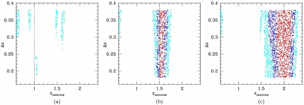
Figure 11. PPM plots for the simulated cluster located in the field of COSMOS-FRI70, with θ = 0 arcsec, and at different redshifts: z = 1.0 (left), z = 1.5 (middle), and z = 2 (right). The dashed vertical line corresponds to the input redshift of the simulated cluster. Overdensities: ⩾2σ (cyan points), ⩾3σ (blue points), and ⩾4σ (red points). A Gaussian filter to eliminate high frequency noisy patterns is applied.
Download figure:
Standard image High-resolution imageIn particular, the cluster at zc = 1.5 and zc = 2.0 is detected with significances of 3.7σ and 4.7σ, respectively. The estimated redshifts are z = 1.56 and z = 2.00, respectively. The estimated sizes are rmax = 86.6 arcsec and rmax = 70.7 arcsec, which correspond to 1.9 Mpc and 1.8 Mpc (comoving), at the estimated cluster redshifts, respectively.
Interestingly, both the redshift and size of these overdensities fully agree with the input parameters of our simulations. All these results further confirm that the PPM is very effective in finding clusters and rich groups and in estimating their properties such as redshift and size, if the projected cluster coordinates are known. In the following we will test the PPM against simulations in the case where the projected cluster coordinates are known with an accuracy of 100 and 200 arcsec.
5.2. Increasing the Offset θ
We repeat all 54 simulations for increasing offsets θ between the input coordinates of the PPM and the center of the simulated cluster. In order to do so, we shift the coordinates of cluster members by θ = 100 arcsec. We keep unchanged both the PPM input cluster equatorial coordinates and the equatorial coordinates of the adopted ECF. As explained above, this is because the surroundings of the ECFs might host dense regions in the redshift range of our interest. In Table 3 we summarize our results, where θ = 100 arcsec, analogous to what is reported in Table 2 for the case of null offset θ.
Table 3. Simulated Cluster Detections (θ = 100'' Offset)
| Rc | Nc = 10 | Nc = 30 | Nc = 60 | Nc = 100 | Nc = 150 | Nc = 200 | ||||||||||||
|---|---|---|---|---|---|---|---|---|---|---|---|---|---|---|---|---|---|---|
| (Mpc) | zc = 1 | 1.5 | 2 | 1 | 1.5 | 2 | 1 | 1.5 | 2 | 1 | 1.5 | 2 | 1 | 1.5 | 2 | 1 | 1.5 | 2 |
| 1.0 | 0/6 | 1/6 | 1/6 | 0/6 | 3/6 | 6/6 | 2/6 | 5/6 | 5/6 | 4/6 | 5/6 | 6/6 | 6/6 | 6/6 | 5/6 | 6/6 | 6/6 | 6/6 |
| 2.0 | 1/6 | 1/6 | 0/6 | 0/6 | 3/6 | 5/6 | 2/6 | 5/6 | 6/6 | 2/6 | 5/6 | 5/6 | 6/6 | 6/6 | 6/6 | 6/6 | 6/6 | 6/6 |
| 3.0 | 0/6 | 0/6 | 0/6 | 0/6 | 2/6 | 4/6 | 1/6 | 3/6 | 5/6 | 3/6 | 6/6 | 6/6 | 4/6 | 6/6 | 6/6 | 6/6 | 6/6 | 6/6 |
Notes. Detection results for the simulated clusters with different input richness (Nc), redshift (zc), and size (Rc), in the case where (1) the equatorial coordinates at which we choose to center the tessellation of the PPM, (2) the equatorial coordinates of the adopted ECF, and (3) the equatorial coordinates of the center of the spherically symmetric simulated cluster do not coincide. We fix the offset θ = 100 arcsec between (1) and (3), changing the equatorial coordinates of the center of the spherically symmetric simulated cluster, while (1) and (2) still coincide. Column description: (1) comoving size (Mpc) of the simulated cluster; (2–13) detection rates for simulated clusters of different richnesses Nc and redshift zc. Each fraction n/6 denotes that the cluster is detected in n out of the six adopted ECFs.
Download table as: ASCIITypeset image
For θ > 100 arcsec the PPM becomes highly inefficient mainly because of the constraint applied to an angular separation of ∼2 arcmin from the coordinates at which the PPM tessellation is centered. In fact, for θ = 200 arcsec, the simulated clusters are all detected in less than five ECFs. Only four high-redshift (zc = 1.5), rich (Nc ⩾ 60), and extended (Rc ⩾ 2 Mpc) clusters are detected in at least three ECFs. Among the four, only the cluster with zc = 1.5, Nc = 200, and Rc = 3 Mpc is detected in four ECFs. This is not surprising. In fact, for such a high value of θ, very extended and rich structures have more chances to be detected.
Note that by considering all the possible combinations of the parameters (i.e., the different ECFs, the offsets, and the different values for Nc, Rc, and zc), 972 clusters are simulated as part of this work.
5.2.1. General Results and Trends
Our simulations suggest that the great majority, i.e., 30 out of the 41 clusters that are detected in at least five ECFs in the case where θ = 0 arcsec, are also found in at least five ECFs if θ = 100 arcsec. Note that 23 out of the 30 clusters have Nc ⩾ 60 and zc > 1 (see Table 3).
For the 30 simulated clusters, the redshift zPPM estimated by the PPM is fully consistent with the input simulated cluster redshift zc. In fact, the average mismatch for the 30 clusters, in the case where θ = 100'' is 〈zPPM − zc〉 = 0.02 ± 0.07, where all detections for the 30 clusters are considered and the reported uncertainty is the rms dispersion around the average. Therefore, the statistical 1σ uncertainty for our redshift estimates is ∼0.07, estimated with Gaussian propagation of the mean offset with the rms dispersion. Interestingly, this is again fully consistent with the independent redshift estimate uncertainties (∼0.06–0.09) described throughout the PPM procedure.
Furthermore, note that poorer overdensities or clusters of intermediate richness (i.e., Nc ⩽ 60) are more difficult to detect than richer clusters. This is especially true at redshift zc = 1.0 and in the case of θ = 100 arcsec, where Nc = 100 cluster members or more are required, unsurprisingly. At variance with the case of null offset (i.e., θ = 0 arcsec), poor and intermediate richness clusters are more difficult to detect by the PPM at such a high offset θ = 100 arcsec. This in fact corresponds to a comoving distance of 1.6 Mpc, at redshift zc = 1.0, which is comparable to the input ∼megaparsec size of the simulated clusters.
Among the 18 clusters with intermediate richness, i.e., Nc = 30 and 60, seven are detected in at least five ECFs. Six among the seven have zc ⩾ 1.5 and Rc ⩽ 2 Mpc.
Rich simulated clusters with Nc ⩾ 100 are always detected at zc ⩾ 1.5 in at least five ECFs. At zc = 1.0, these rich clusters are detected with more difficulty, especially in the case Nc = 100, while they are detected in at least four ECFs if they have Nc ⩾ 150.
5.2.2. Detection Significances
The overdensities found in the case of θ = 100 arcsec are detected, by construction, with significances ⩾2σ, and a median value of 3.9σ. Therefore, the overdensities tend to be detected with lower significances than in the case of θ = 0 arcsec.
In particular, for θ = 100 arcsec and similarly to what is found in the case of null offset, at fixed size and richness, the clusters are detected with increasing significances for increasing redshifts. However, at variance with the case θ = 0 arcsec, at each fixed richness and redshift, no specific trend is observed for the detection significances, for increasing sizes Rc. This is because of two competing effects: a larger sized cluster is more easily detected than more compact overdensities, at a larger offset θ. On the contrary, similarly to what was discussed in the case of null offset θ = 0 arcsec, a larger size implies a lower projected number density that makes the cluster detection more difficult.
5.2.3. Projected Cluster Sizes
The comoving cluster size estimated by the PPM as rmax in the case where θ = 100 arcsec is ∼1.6 times the input comoving cluster size Rc (and up to a factor of ∼2.6 at 1σ). The reason for this mismatch is due to the fact that, by construction, the simulated cluster formally ends at a larger distance from the input PPM coordinates than in the case of θ = 0 arcsec.
These aspects suggest that, if the coordinates of the cluster center are not accurately known, the cluster sizes might be overestimated by up to a factor of ∼2.6, which corresponds to the extreme case where we are looking for a cluster environment around a radio source that resides in the outskirts of the cluster core.
6. SUMMARY AND CONCLUSIONS
The goal of this project is to search for high-redshift z ≳ 1 clusters or groups using FR I radio galaxies as beacons. In this paper, we have introduced a new method we developed to achieve such a goal. The method is tailored to the specific properties of the z ∼ 1–2 FR I radio galaxy sample we consider (Chiaberge et al. 2009), selected within the COSMOS survey (Scoville et al. 2007b), and to the specific data set used.
The PPM is adapted from the method proposed by Gomez et al. (1997) to search for X-ray emitting substructures within clusters in the low number count regime. Here we are similarly dealing with the problem of small number densities.
We test the efficiency of the PPM in searching for cluster candidates against simulations. Two different approaches are adopted. (1) We use two z ∼ 1 X-ray detected clusters found in the COSMOS survey within the Finoguenov et al. (2007) catalog. We shift them to higher redshift up to z = 2. We find that the PPM detects both clusters up to z = 1.5, and it correctly estimates both the redshift and the size of the two clusters. (2) We simulate spherically symmetric clusters of different size and richness, and we locate them at different redshifts (i.e., z = 1.0, 1.5, and 2.0) in the COSMOS field. We find that the PPM detects the simulated clusters within the entire redshift range considered with a statistical 1σ redshift accuracy of ∼0.05. This is remarkably comparable to the statistical photometric redshift uncertainty of photometric redshift catalogs over the same redshift range (Mobasher et al. 2007; Ilbert et al. 2009).
Our results suggest that almost all of our simulated clusters are detected. Compact clusters (i.e., 1 Mpc comoving size) and rich clusters are more easily detected than lower richness clusters, when the cluster center coordinates are accurately known. The majority of these clusters are also detected even if the coordinates of the cluster center are known with a poor accuracy of ∼100 arcsec. Furthermore, poor overdensities and clusters of intermediate richness are more difficult to detect in the case where the cluster coordinates are known with an accuracy of ∼100 arcsec. Concerning cluster sizes, we found that the PPM provides estimates with a 33% rms fractional accuracy if the cluster center coordinates are known.
We applied the Kolmogorov–Smirnov (KS) test to the cumulative number distributions of galaxies in the fields of the Chiaberge et al. (2009) sample similarly to what was done in previous work on COSMOS (e.g., Harris 2012). We checked that the KS test is ineffective in dealing with these types of cluster searches and the results are not conclusive. This is because shot noise fluctuations affect the results of the KS test.
We found that our method is effective in finding clusters up to high redshift. We believe that the PPM is a valuable alternative to previously considered methods to search for high-redshift clusters based on photometric redshifts. In fact, with the inclusion of a solid positional prior and an accurate redshift sampling, we overcome, at least in part, the problem of establishing whether multiple overdensity peaks in the 2D projected density field are part of a single larger structure (Scoville et al. 2013) and, thus, identifying different structures at different redshifts.
Although the PPM is primarily introduced for the COSMOS survey (see Paper II), it may be applied to wide field surveys to blindly search for cluster candidates. Accurate photometric redshifts and a survey depth similar to or better than that of COSMOS (e.g., I < 25) are required.
However, our method is less effective for those surveys that will provide sufficient spectroscopic redshift information, where standard 3D methods such as correlation functions might be more successfully applied. Conversely, the PPM might also be applied to SDSS Stripe 82 and future wide field surveys, such as LSST and Euclid, that will provide accurate photometric redshift information. Another possible use of the PPM is to search for (proto-)clusters at z ≳ 2, by adopting radio galaxies or other sources such as Lyman break galaxies as beacons.
We are grateful for useful comments from an anonymous referee. We thank the Space Telescope Science Institute, where part of this work was developed. We also thank Gianfranco De Zotti, Roberto Gilli, Piero Rosati, and Paolo Tozzi for fruitful discussion. This work was partially supported by the STScI JDF account D0101.90157, and (G.C.) by both the Internship Program ISSNAF-INAF 2010 and one of the Foundation Angelo Della Riccia fellowships both in 2012 and in 2013.
APPENDIX: THE POISSON PROBABILITY METHOD (PPM)
As mentioned in Section 3, the PPM is adapted from the method proposed by Gomez et al. (1997, see their Appendix A) to search for X-ray emitting substructures within clusters. We introduce such a method to search for the presence of clusters in a given field, around specific projected coordinates, by using photometric redshift information. Therefore, our method is not properly a method to search for cluster candidates but to verify their presence around a given beacon (this is an approach similar to that adopted by previous work, e.g., George et al. 2011).
The method we describe in the following is tailored to the specific properties of the sample and data set used, to which we refer throughout the method description. More specifically, the PPM has been introduced to search for cluster candidates around z ∼ 1–2 FR Is selected in the COSMOS field (Scoville et al. 2007b) by Chiaberge et al. (2009). We also use photometric redshifts from the Ilbert et al. (2009) catalog.
The PPM is based on photometric redshifts and galaxy number counts. Similarly to other methods that use photometric redshift information (e.g., Eisenhardt et al. 2008), we consider the redshift information and the coordinates in the projected space separately. This is because the photometric redshift uncertainties are much larger than the typical scale of clusters. Therefore, such uncertainties are significantly dominant with respect to any other observable uncertainty (e.g., flux uncertainties, projected space coordinate uncertainties). In the following we will focus first on the projected space and then on the redshifts.
A.1. The Projected Space
We tessellate the projected space with a circle centered at the coordinates of the beacon (in our specific case this is the location of the FR I radio galaxy) and 49 consecutive adjacent annuli. These regions are concentric and have the same area, i.e., 2.18 arcmin2. This is done in order to have the same average field density for each of the regions. The inner radius of the i-th annulus is equal to ![$\arccos [1+i(-1+\cos 50\, {\rm arcsec})] \simeq 50\times \sqrt{i}$](https://content.cld.iop.org/journals/0004-637X/792/2/113/revision1/apj497870ieqn12.gif) arcsec. This means that the radius of the circle centered at the coordinates of the beacon is equal to 50 arcsec. Such an angular separation is consistent with that adopted in previous work focused on high-z clusters (e.g., Santos et al. 2009; Adami et al. 2010, 2011; Durret et al. 2011; Galametz et al. 2012; Spitler et al. 2012). In fact, it corresponds to 427 kpc at redshift z = 1.5, which is typical of the cluster core size at redshift z ∼ 1. If we chose a smaller scale, we would be highly affected by shot noise. In fact, on average, for a fixed area of 2.18 arcmin2, the differential number counts (dN/dz) per unit redshift in the COSMOS field are quite small and equal to ∼55, 22, and 7, at redshifts z ≃ 1, 1.5, and 2.0, respectively (Ilbert et al. 2009). Conversely, if we chose a greater scale, we would characterize the cluster environment of the FR Is in our sample with rough (megaparsec-scale) accuracy only.
arcsec. This means that the radius of the circle centered at the coordinates of the beacon is equal to 50 arcsec. Such an angular separation is consistent with that adopted in previous work focused on high-z clusters (e.g., Santos et al. 2009; Adami et al. 2010, 2011; Durret et al. 2011; Galametz et al. 2012; Spitler et al. 2012). In fact, it corresponds to 427 kpc at redshift z = 1.5, which is typical of the cluster core size at redshift z ∼ 1. If we chose a smaller scale, we would be highly affected by shot noise. In fact, on average, for a fixed area of 2.18 arcmin2, the differential number counts (dN/dz) per unit redshift in the COSMOS field are quite small and equal to ∼55, 22, and 7, at redshifts z ≃ 1, 1.5, and 2.0, respectively (Ilbert et al. 2009). Conversely, if we chose a greater scale, we would characterize the cluster environment of the FR Is in our sample with rough (megaparsec-scale) accuracy only.
In general, due to the specific tessellation of the PPM, the method is effective in detecting megaparsec-scale rich groups and clusters (as also discussed in Paper II). Conversely, it might be less efficient in finding poor groups and larger, i.e., a few megaparsec-scale, diffuse structures. Therefore, a more detailed treatment of the projected space typical of sophisticated tessellations such as Voronoi–Delaunay (see, e.g., Ebeling & Wiedenmann 1993) correlation estimators (e.g., Adami et al. 2011), wavelet analysis (e.g., Eisenhardt et al. 2008), filter techniques, and adaptive kernels (e.g., Scoville et al. 2007a) might be ineffective and difficult to apply for cluster searches with the use of photometric redshifts only (see also Scoville et al. 2013, for further discussion). On the other hand, such methods might be more useful to study spectroscopically confirmed clusters or groups (e.g., Jelić et al. 2012).
The typical size inspected by our tessellation changes at most ∼6% within the entire redshift range of our interest. In fact, 1 arcmin corresponds to a physical size of 482, 512, and 509 kpc at redshift z = 1.0, 1.5, and 2.0, respectively. Depending on the adopted cosmology, the angular distance assumes a maximum between z ∼ 1–2. These considerations imply that our tessellation is effective at characterizing megaparsec-scale overdensities with the required accuracy, independently of redshift, under the assumption that cluster core size does not dramatically change for increasing redshifts.
Furthermore, our approach implicitly assumes azimuthal symmetry around the axis oriented at the coordinates of the beacon. We do not exclude the possibility of detecting non-circularly symmetric systems, since we extend the tessellation up to ∼6 arcmin (i.e., ∼3 Mpc at z = 1.5) from the coordinates of the beacon (Postman et al. 1996). Moreover, our method is also flexible enough to find clusters even if the coordinates of the cluster center are known within ∼100 arcsec only (as tested with simulations in Section 5.2).
However, we note that the great majority of low-power radio sources in clusters or groups are found within ∼200 kpc from the core center up to z ≃ 1.3 (Ledlow & Owen 1995; Smolčić et al. 2011). Therefore, this suggests that low-power radio galaxies in cluster environments are preferentially hosted within the central regions of the core, at least at low or intermediate redshifts. The results presented in the companion paper (see discussion in Section 8.8 of Paper II) for the z ∼ 1–2 cluster candidates within the Chiaberge et al. (2009) sample suggest that this is generally true also at higher redshifts. Therefore, all these results support the specific projected space tessellation method described in this section and adopted for our cluster search.
A.2. Redshift Information
As discussed in Scoville et al. (2007a), identifying large-scale structures on the basis of 2D number densities requires a careful selection of those galaxies that are at the redshift of the structure. This is because, especially in the case of high-z clusters, foreground galaxies contaminate the field. Despite this, the contamination from foreground sources is limited by the smaller angular size of high-z clusters with respect to the contamination of those at lower redshifts.
As pointed out in Scoville et al. (2007a), three different criteria are commonly adopted to discriminate among the galaxies at different distances by using (1) color selections (e.g., Papovich 2008; Gladders & Yee 2005), (2) spectroscopic redshifts (e.g., Knobel et al. 2009, 2012; Diener et al. 2013), or (3) photometric redshifts (e.g., Adami et al. 2010; Durret et al. 2011).
(1) Color selection is not used here since it might be biased toward large-scale structures with specific properties in terms of galaxy colors. This is particularly important especially at redshift z ≳ 1.5, where the properties of the cluster galaxy population and their changes with redshift in terms of galaxy morphologies, types, masses, colors (e.g., Bassett et al. 2013; McIntosh et al. 2014), and star formation content (e.g., Zeimann et al. 2012; Santos et al. 2013; Strazzullo et al. 2013; Gobat et al. 2013) are still debated. (2) Spectroscopic redshifts are preferred to the photometric redshifts. However, spectroscopic redshift catalogs (e.g., Lilly et al. 2007) are limited to a small fraction of the galaxies in the COSMOS field. (3) We adopt the photometric redshift catalog of Ilbert et al. (2009), which was obtained considering sources with AB magnitude I < 25.
We consider M ≫ 1 redshift bins, i.e., the closed intervals ![$[z_l^i, z_r^i]$](https://content.cld.iop.org/journals/0004-637X/792/2/113/revision1/apj497870ieqn13.gif) , with
, with  , i = 1, 2,..., M, and M = 22,500. We define the length and the centroid of each interval as
  and
and  , respectively. The subscripts l and r stand for left and right, respectively. Both the redshift lengths Δzi ∈ [0.02; 0.4] and the redshift centroids
 ![$z_{\rm centroid}^i\in [0.4;4.0]$](https://content.cld.iop.org/journals/0004-637X/792/2/113/revision1/apj497870ieqn17.gif) are randomly and independently chosen assuming a uniform distribution. Since M ≫ 1, the considered ranges are densely spanned in terms of both the redshift bin and the redshift centroid. The redshift range of our interest is z ∼ 1–2, while the typical statistical photometric redshift uncertainties at those redshifts are σz ∼ 0.1–0.2 (Ilbert et al. 2009). Therefore, both Δzi and
are randomly and independently chosen assuming a uniform distribution. Since M ≫ 1, the considered ranges are densely spanned in terms of both the redshift bin and the redshift centroid. The redshift range of our interest is z ∼ 1–2, while the typical statistical photometric redshift uncertainties at those redshifts are σz ∼ 0.1–0.2 (Ilbert et al. 2009). Therefore, both Δzi and  are conservatively selected over wider intervals than those of our interest. This is done in order to avoid spurious boundary effects that might derive from our selection. Before describing in detail our method in the following section we will discuss its theoretical framework.
A.3. Theoretical Framework
We denote by n the galaxy number density within a given projected area of the sky subtended by a solid angle Ω. The total variance in the number counts n is given by Peebles (1980)
where
is the sampling variance due to source clustering. As pointed out in, e.g., Massardi et al. (2010),  adds a significant contribution to the uncertainties in the case of small-area fields. As pointed out in Peebles (1980), assuming ergodicity, the average denoted by the brackets
  is either the ensemble average (i.e., the average among all the field realizations) or the volume average (i.e., the average among different areas in the survey, each of them is subtended by a solid angle Ω). The clustering term in Equation (A2) is expressed as the integral over the field of the projected two-point correlation function ω(θ), where θ is the angular separation between the solid angle elements dΩ1 and dΩ2.
We note that n would be Poisson distributed if the clustering term were not present. Then, we ask what is the probability that the null hypothesis (i.e., no clustering) occurs for the given field. This is equivalent to set  and to assume that n is Poisson distributed. According to our formalism, we estimate the probability of not clustering as the probability to have a number density n' equal to or higher than the observed value n:
As for Equation (A1), 〈n〉 and Ω are the average number density for the survey considered and the solid angle subtended by the selected field for which we estimate the null hypothesis probability, respectively. Therefore, the null hypothesis is rejected with a probability
The probability  is higher in those fields where the sources are more clustered, i.e., where
  is non-negligible with respect to the shot noise term 1/〈n〉. Therefore,
  can be independently considered in this paper as the probability that an overdensity is present in the field.
So far, our formalism implicitly assumes that the sample selection is a negligible source of uncertainty (i.e., it does not contribute to the total variance of Equation (A1)). However, the cluster membership selection (based on, e.g., fluxes, colors, or redshifts) always contributes to the total number count variance because of the observable uncertainties. Equivalently, observable uncertainties imply that the total variance in Equation (A1) is underestimated. Consequently, Equation (A4) overestimates the probability  that the null hypothesis (i.e., no overdensity) is rejected.
Limiting the analysis to the PPM, our method is based on number counts and photometric redshifts. According to the PPM procedure, for each redshift bin Δzi, only those sources within the redshift interval ![$[z_l^i, z_r^i]$](https://content.cld.iop.org/journals/0004-637X/792/2/113/revision1/apj497870ieqn26.gif) are considered (see below, Section A.4). Photometric redshift uncertainties are significantly higher than those of any other observable (e.g., flux, projected coordinates) associated with our sample.
are considered (see below, Section A.4). Photometric redshift uncertainties are significantly higher than those of any other observable (e.g., flux, projected coordinates) associated with our sample.
This implies that we can estimate the additional term in the number count variance in Equation (A1) due to observable uncertainties by considering photometric redshift uncertainties only. We denote such a term as  , where the notation ph stands for photometric redshifts. This term can be independently estimated as the number count variance obtained by averaging over all the possible realizations of the photometric redshifts of the galaxies in the selected field. These realizations are ideally drawn from the redshift probability distributions of the galaxies in the field. Hence, we have
where  denotes the average over the ensemble constituted by all the possible redshift realizations. The net effect of increasing the number count variance in Equation (A1) by the amount
  is similar to that described in, e.g., Sheth (2007) in the context of luminosity functions estimated by adopting photometric redshifts. Sheth (2007) showed that photometric redshift uncertainties (i.e., distance errors) have the effect of scattering objects to the low-luminosity and high-luminosity ends of the luminosity function (i.e., toward higher and lower luminosities). Similarly, in our case, photometric redshift uncertainties have the effect of scattering the number counts over a wider range.
Given the additional term  in the right hand side of Equation (A1), a rigorous calculation of the probability of the null hypothesis (i.e., no clustering,
  ) would require us to consider the redshift probability distribution associated with each galaxy in the field. Estimating the correct expression of the null hypothesis probability might be done with simulations, i.e., adopting different realizations of the redshifts, which are drawn from the redshift probability distribution associated with each galaxy in the field. However, this procedure would be enormously demanding in terms of time and would not add a significant contribution to the PPM. We prefer to adopt a different approach. We neglect any additional terms in the number count variance due to observational uncertainties. We prefer to take into account such an approximation by correcting our final estimate (see Section A.5). Our correction will decrease the probability
  . In the next sections we will describe how our method works.
A.4. The Method
First, we consider each pair defined by the redshifts  and
and  , as in Section A.2, and the sources in the Ilbert et al. (2009) catalog that have redshifts within the interval
  and that fall within the largest circle that can be inscribed in the COSMOS survey. Such a circle subtends a ∼1.25 deg2 solid angle. Then, we estimate the average mean density 〈n〉i as the ratio of the number of these sources to the solid angle subtended by the circle. We test if cosmic variance affects our analysis by adopting different choices in estimating such an average number density (i.e., we also selected four disjoint quadrants in the COSMOS survey and we estimated the average number density for each quadrant, separately). We verified that the results are independent of the choice adopted.
For a given beacon, in our case the projected coordinates of the radio galaxy, we consider each of the 50 projected regions defined in Section A.1. We denote them with the index t = 1, ..., 50, where t = 1 corresponds to the central circle, while the adjacent annuli are denoted with progressively higher indexes. We denote by  the observed number of galaxies within the chosen redshift interval
  that fall within the t-th area. By construction, each region subtends a solid angle ΔΩt = 2.18 arcmin2. We also define the observed number density for the selected region and redshift bin as
  . The probability of a null hypothesis (i.e., no clustering) for the t-th region, consistent with Equation (A3), is
which corresponds to the probability of having a number density  higher than or equal to the observed one, according to the Poisson statistics. Note that, because of the low number counts, the Gaussian statistics is not a good approximation of the Poisson statistics, and therefore the latter is required.
Starting from the central region corresponding to t = 1 we select the first adjacent regions, denoted with the indexes  , for which the probability of the null hypothesis in Equation (A6) is ⩽30%. Here
  and hi ⩾ 0 are both integer numbers. Note that we do not exclude the possibility of selecting one single region, i.e., hi = 0. The central circle may be selected or not, depending on whether the threshold criterion is satisfied or not by that region.
According to our prescription, we have selected only those regions for which the null hypothesis is rejected at a level of ⩾70%, i.e., down to about 1σ. Note that the adopted ∼1σ threshold is not a tight constraint. A 70% threshold is also adopted by Gomez et al. (1997) and is similar to the values adopted for other selection criteria applied by previous papers that were focused on high-z clusters and that used photometric redshift information (e.g., Papovich et al. 2010; Finkelstein et al. 2010).
According to the procedure, the probabilities are always estimated according to Poisson statistics. Even if the Gaussian statistics are not adopted we often refer to the probability in terms of σ (e.g., we refer to 68.27%, 95.45%, and 99.73% probabilities as 1σ, 2σ, and 3σ significances, respectively). We adopt this notation for practical reasons, for sake of convenience.
Similar to what was done in Gomez et al. (1997), in order to determine the true significance of the number count excess in the field, we merge together all the hi + 1 adjacent regions to form a (larger) circle or an annulus, depending on whether the central circle is included or not, respectively. Then, we define the total observed number count Ni for the new region as
and the corresponding number density ni as
We stress that the goal of the procedure described so far is not to quantify the number count excess associated with the field. Merging the hi + 1 regions aims at selecting an area in the projected space for which there is indication of a number count excess and that is most likely associated with the projected coordinates of the beacon.
Note that if we chose a more constraining (i.e., >1σ) threshold criterion, we would select only those regions that show a significant number count excess. Therefore, we might be biased toward selecting those regions (1) that are associated with highly overdense substructures in the cluster or (2) show high shot noise fluctuations. These scenarios might occur because of the small area subtended by each region (i.e., ∼2 arcmin2) and the small number densities that occur at the redshifts of our interest. This discussion suggests that a more constraining (i.e., >1σ) criterion might not be effective in selecting properly the cluster field in the projected space.
Then, analogously to what was done for each of the 50 regions (see Equation (A6)), we estimate the probability of a null hypothesis (i.e., no clustering) for the new area as
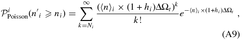
which is the probability of having a number density n'i higher than or equal to that observed, ni, according to the Poisson statistics. For the sake of clarity, hereafter we omit the argument of  . We also define
  and
and  as the minimum and maximum projected distances, respectively, from the coordinates of the beacon (in our case it is the radio galaxy) within which the number count excess is detected. These radii are equal to
 ![$r_{{\rm min}}^i=\arccos [1+(\overline{t}_i-1)\times (-1+\cos 50\, {\rm arcsec})]\simeq \sqrt{\overline{t}_i-1}\times 50$](https://content.cld.iop.org/journals/0004-637X/792/2/113/revision1/apj497870ieqn45.gif) arcsec and
arcsec and ![$r_{{\rm max}}^i=\arccos [1+(\overline{t}_i+h_i)\times (-1+\cos 50\, {\rm arcsec})] \simeq \sqrt{\overline{t}_i+h_i}\times 50$](https://content.cld.iop.org/journals/0004-637X/792/2/113/revision1/apj497870ieqn46.gif) arcsec, because of the specific tessellation, consistent with the adopted procedure.
arcsec, because of the specific tessellation, consistent with the adopted procedure.
According to what was discussed in Section A.3, the null hypothesis is rejected with a probability  . We set
  if the overdensity starts to be detected from rmin ≳ 132 arcsec, i.e., if
  . This is done to reject those overdensities that are detected only at large angular separation from the location of the source. In fact, since 132 arcsec corresponds to ∼1.1 Mpc at z = 1.5, these overdensities might not be associated with our beacon. However, note that such a constraint does not exclude the possibility of detecting structures that are extended up 132 arcsec or even higher. These extended structures are detected if they start at a distance lower than 132 arcsec.
The specific projected distance of 132 arcsec corresponds to 0.8 h−1 Mpc (h = 0.71), which is the scale where the amplitude of the correlation function between radio loud AGNs and luminous red galaxies is reduced to a few percent (∼4%) of the value at its maximum, up to z ≃ 0.8 (e.g., Donoso et al. 2010; Worpel et al. 2013).
Limiting the number counts to the hi + 1 overdense regions between the radii  and
and  does not bias our results toward overestimating the number count excess because we are allowed to select slightly overdense regions, down to ∼1σ number count excess.
Similarly, the probability of detecting those fields that show low number count excess or shot-noise fluctuations is negligible. This is because the number of selected galaxies does not decrease when the hi + 1 regions are merged and then the number count excess probability is re-estimated for the new (larger) region delimited by the radii  and
and  . We will describe in the following sections the noise mitigation procedure and the peak finding algorithm adopted to detect overdensities. As will be clarified below, both of these procedures further suppress the probability of detecting as overdensity any number count excess that is simply due to shot noise fluctuations.
A.5. Noise Mitigation
In Figure 12, left panel, we plot  as a function of the redshift bin Δz and its centroid zcentroid. We omit the index i corresponding to the specific redshift interval. We will introduce such an index only where necessary. Red, blue, and cyan colors refer to points with significances ⩾4σ, ⩾3σ, and ⩾2σ, respectively. We plot as a vertical solid line the spectroscopic redshift of the source.

Figure 12. PPM plots for source 01. Left: no filter is applied. Right: the Gaussian filter which eliminates high frequency noisy patterns is applied. The abscissa of the vertical solid line is at the spectroscopic redshift of the source. We plot only the points corresponding to detected overdensities for different values of Δz and zcentroid. Color code: ⩾2σ (cyan points), ⩾3σ (blue points), ⩾4σ (red points).
Download figure:
Standard image High-resolution imageIsolated high significance spiky patterns are clearly visible in the plot. They occur because of the presence of a significant source number excess at specific redshifts and redshift bins. However, the fact that such patterns are spiky and extended over scales that are smaller than the typical statistical photometric redshift uncertainties (σz ∼ 0.1–0.2) suggests that they are not physical and are ultimately due to noise fluctuations.
In order to eliminate such high frequency noisy patterns, we apply a Gaussian filter to the function  as follows:
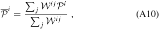
where the kernel
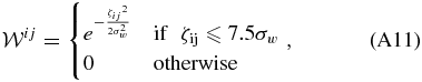
and

For practical reasons, the sum over j is extended only to those points that are at most 7.5σw from ( ; Δzi), so that the kernel has a compact domain and acts as a weighted local average. The newly defined function,
  , is simply the convolution between the Gaussian filter and the previously defined probability
  .
.
In practice, patterns that are extended over scales of the order of ≲ σw with respect to zcentroid or Δz are removed from the plots. We choose σw = 0.02, which is much lower than the typical statistical photometric redshift uncertainty σz ∼ 0.1–0.2 of the Ilbert et al. (2009) catalog. Therefore, our choice conservatively removes those patterns that are clearly due to noise.
Isolated local maxima are removed from the plots since they are suppressed by the surrounding low significance points. Conversely, local maxima that belong to extended high significance patterns still remain associated with high significance patterns, even if their significance is decreased because of the average procedure.
A heuristic physical interpretation may be provided. Averaging  among those points that belong to the neighborhood of zcentroid and Δz mimics the presence of the redshift uncertainties at fixed zcentroid and Δz. This is because changing zcentroid and Δz by small amounts has the net effect of including some sources and excluding others when the redshift interval is changed. To understand better such a heuristic equivalence, in the following we will adopt a variational approach.
We note that  can be naturally interpreted as an effective mean field defined on the space of (
 ; Δzi). This is because the incoherent fluctuations of
  due to noise and at small scales are locally suppressed by the filter
  .
.
There is no theoretical and observational reason to prefer one specific form for the kernel  . In the effective field theory context, since the width of the filter is related to the statistical photometric redshift uncertainties, it is more relevant than the specific shape of the filter
  . In fact, the Gaussian filter is chosen because its exponential declining assures that noisy features associated with scales (that are smaller than the typical statistical photometric redshift uncertainty) are conservatively removed.
A more physical interpretation of the filtering procedure described in this section may be provided by using a variational approach. Several methods of analysis of functionals of Poisson processes, including variational calculus, have been developed in the context of stochastic analysis (e.g., Privault 1994; Albeverio et al. 1996; Molchanov & Zuyev 2000). We stress that the following discussion does not intend to be a formal proof but simply an argument that shows how we can assign a physical meaning to the  values and, thus, better explain the abovementioned heuristic equivalence that arises when the filtering procedure is reconsidered. A more detailed analysis will be performed in a forthcoming paper.
We adopt a compact notation and we define the vector  ; Δz) whose i-th component is given by (
 ; Δzi). We consider the galaxies that are in the field of our beacon (i.e., the radio galaxy in our case) and whose redshifts belong to a neighborhood of the redshift zcentroid corresponding to the specific
  . The values of Δz and zcentroid can be expressed as the redshift range spanned by the selected galaxies and the redshift centroid of that redshift range, respectively. This implies that the value of
  at
at  ultimately depends on the set {zj} of the redshifts of the galaxies in the field of the beacon, where each set {zj} is selected in such a way that the corresponding (zcentroid; Δz) belongs to a neighborhood of
  . This argument shows that
  is a function of {zj} and, therefore,
  is a function of {zj}, i.e.,
  .
.
Each set {zj} is a specific realization of the photometric redshifts. Each set belongs to the ensemble constituted by all the possible redshift realizations. These realizations are ideally drawn from the redshift probability distributions of the galaxies in the field of the beacon.
Since  is not an analytic function, first we assume that
  is defined on a discrete domain, given by the points in Figure 12 (left panel), then we consider a local analytic first-order approximation of
  at
at  . By construction, the analytic approximation has a local continuous domain. For the sake of simplicity, in the following we do not distinguish
  from its analytic approximation. Adopting the analytic approximation allows us to use a variational approach16 and expand
  in Taylor series as follows:
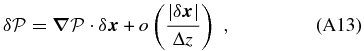
where  is the variation of
  induced by the variation
  .
.
The first term in the right hand side (rhs) of the equation is the scalar product of the variation  and the gradient
  of
of  with respect to
  .
.
We stress that it is not straightforward to provide an explicit expression for all the terms in the Taylor series.17 In fact, the explicit expression depends on the specific number counts in the field, the specific redshift zcentroid, and redshift bin Δz. We checked that finite differences  of
of  corresponding to small displacements
  in the PPM plots (e.g., in Figure 12, left panel) satisfy the relation
  for almost all of the ⩾2σ points in the plot (except for a negligible set). This argument leads to the term
  in Equation (A13) and implicitly implies that only those points associated with high significance (i.e., ≳ 2σ) patterns are considered. This constraint does not affect our analysis. In fact, as outlined below, only these patterns may be ultimately associated with cluster detections.
The variation  at
at  can be alternatively estimated as follows. Limiting our analysis to a neighborhood of
  and to the field of the beacon, analogously to what was done in Equation (A13), we estimate the variation
  of
of  induced by the variations of {zj} within the ensemble as follows:
where the sum over j is restricted to a neighborhood of  as specified above and to the galaxies in the field of the beacon. The subscript ph stands for photometric redshifts and it is introduced to distinguish the variation
  from
from  . The first and second terms in the rhs of the equation are the first term and the higher order terms of the Taylor expansion, respectively. The second term reported in Equation (A14) is estimated similarly to what was done in Equation (A13). The chain rule is also applied to express the derivatives with respect to zj into derivatives with respect to Δz and zcentroid.
We stress that the variations  and
and  are different;
  is the variation of
  due to small variations δ(Δz) and δzcentroid of the redshift bin and the redshift centroid, respectively. Conversely,
  is the variation of
  due to the photometric redshift uncertainties of the redshifts of the galaxies in the field of the beacon. Equivalently,
  is the variation of
  in the ensemble of all possible redshift realizations of the galaxies in the field of the beacon. Combining Equation (A13) and Equation (A14) we estimate the difference between the two variations of
  as follows:
where the same notation and the chain rule adopted above is used. The equation, combined with the Equations (A13) and (A14), shows that the two variations  and
and  are equal up to the first order in the perturbations.
By construction, the filter  removes the fluctuations of
  on small scales. Because of the exponential declining of the Gaussian filter, it is effective on scales
  . As will be explained below, cluster candidates are selected at the fixed redshift bin Δz = 0.28. This redshift bin corresponds to the estimated statistical 2σ photometric redshift uncertainty at z ∼ 1.5 for dim galaxies (i.e., with AB magnitude i+ ∼ 24; Ilbert et al. 2009).
Therefore,  . This inequality implies that the scales are sufficiently small to assure that the filter
  suppresses the variation
  up to the first order, as in Equation (A13), i.e.,
  .
.
Similarly, the condition  is reasonably satisfied because
  approximately corresponds to the quadratic average of the photometric redshift uncertainties of the galaxies in the field. Such an average is reasonably smaller than the selected redshift bin Δz = 0.28. Therefore, the variation
  in Equation (A14) is well approximated, for our purposes, by the linear expansion.
Resuming, Equations (A13) and (A14), combined with the two reported inequalities, suggest that in our case both  and
and  can be expressed in linear theory. Similarly, Equation (A15), combined with the two inequalities, tells that the two variations are equal in first-order approximation. Therefore this argument suggests that the filter
  simultaneously suppresses (in linear approximation) both the variation
  and variation
  due to the photometric redshift uncertainties.
This discussion suggests that  is a good estimate of the number count excess probability. In fact, as discussed in Section A.3, since the photometric redshift uncertainties add a significant contribution to the total number count variance,
  represents an overestimate of the true detection significance. Our procedure takes into account a posteriori the initial overestimation: the significance of the local maxima is decreased when the filter is applied. Equivalently, the procedure reasonably removes, as required, the excess of
  that is ultimately due to the photometric redshift uncertainties and the corresponding number count variance expressed in Equation (A1).
Note that the parameters adopted here for the Gaussian kernel and those used in the following for the cluster detection procedure are chosen because of the properties of the photometric redshifts of our sample and of the Ilbert et al. (2009) catalog. In particular, the parameters Δz (= 0.28) and σw (=0.02) are finetuned in such a way that the linear perturbation theory (see Equations (A13) and (A14) is reasonably correct in both the two spaces (that of  and the ensemble of all the redshift realizations). In general, all the parameters are adapted to the specific data set used. We verified that our results are independent of a slightly different choice of these parameters. This is ultimately due to the fact that the procedure is not performed on physical observables (e.g., on the density field), but acts directly on the PPM plots as those reported in Figure 12.
In Figure 12, right panel, we plot the values of  as a function of zcentroid and Δz. The same color code for the left panel is adopted. When the Gaussian filter is applied, isolated noisy patterns are substantially removed from the plot, as is clear from visual comparison of the left panel with the right panel in the figure. Furthermore, we observe that triangular-shape high significance (i.e., ≳ 2σ) patterns are still clearly present in the plot. They are stable with respect to different values of Δz, i.e., the patterns are extended along the Δz axis. In particular, they tend to increase their width in the zcentroid direction for increasing Δz. This is due to the fact that for increasing Δz, we are including more and more objects that are far from zcentroid. Therefore, we still detect a number count excess at values of zcentroid that are increasingly far from the true redshift of the overdensity, even if with lower significance. In fact, lower significance is associated with the boundaries of the triangular-shape patterns than that related to the central regions of these patterns.
A.6. Peak Finding Algorithm
In this section we will describe our procedure to detect and characterize the overdensities we find in the considered field by using the PPM plots. These goals will be achieved by finding the local maxima of the function  . The peak finding algorithm we will describe is a specific procedure we developed for our discrete case and it belongs to a more general context known as Morse theory. Such a theory can be used to find and characterize the critical points of differentiable functions defined on a manifold (see, e.g., Guest 2001, for a review). Notably, there are many applications of Morse theory in the context of differential topology (Bott 1960; Milnor 1963) and in quantum field theory (Witten 1982, and following work).
First, since the high significance patterns in the PPM plots are stable with respect to the Δz axis we simplify the problem to a one-dimensional (1D) case as follows. We consider only those points  such that the redshift bins Δzk fall within a tiny δ(Δz) = 0.01 wide interval centered at Δz = 0.28. This redshift bin corresponds to the estimated statistical 2σ photometric redshift uncertainty at z ∼ 1.5 for dim galaxies (i.e., with AB magnitude i+ ∼ 24; Ilbert et al. 2009). These magnitudes are typical of the galaxies we expect to find in clusters in the redshift range of our interest. We verified that our results are stable with respect to a sightly different choice of the redshift bin Δz.
Then, we sort the points {pk} in increasing order of  , and we redefine the ordering of the points in such a way that
  . Hence, our problem is reduced to finding the maxima of
  defined on the 1D discrete domain
  . Having reduced the dimensionality of the domain is a great simplification, since saddle points are not present in the 1D case, where critical points are of only two types: maxima and minima.
Starting from the significance s = 2σ, we select those intervals of consecutive points that have significances ⩾s. We merge consecutive intervals that are separated by δzcentroid = 0.02 or less along the zcentroid axis. We also reject those intervals that are shorter than δzcentroid = 0.1 along the zcentroid axis. The first condition merges those intervals that are separated by a tiny separation along the zcentroid axis. The minimum allowed separation between two consecutive intervals is set equal to the dispersion σw adopted for the filtering procedure. In fact, fluctuations that occur on these scales may not be physical since they occur for redshift separations that are well below those of typical statistical redshift uncertainties. Similarly, the second condition is applied in order to detect only high significance features whose length along the zcentroid axis is at least comparable with the typical statistical photometric redshift uncertainty of the Ilbert et al. (2009) sample. Given the significance s, this procedure gives a set of intervals that we define as s intervals.
Then, we increase the significance threshold by a tiny amount ds = 0.1σ and we repeat the above outlined procedure. We note that each (s + ds) interval is entirely included within an s interval. We retain those s intervals that do not contain any (s + ds) interval, whereas we reject all the other s intervals.
The significance s is increased and the procedure is repeated until no s interval is found. The final set of s intervals represents the local maxima of  . These intervals have different significances s and they are centered at different redshifts zcentroid. Each s interval corresponds to a cluster candidate detection and is associated with a number count excess found in the given field and around a specific redshift. In Figure 13 we show a visual representation of the peak finding algorithm adopted. In the following section we will describe how the method estimates cluster properties such as the redshift and size.
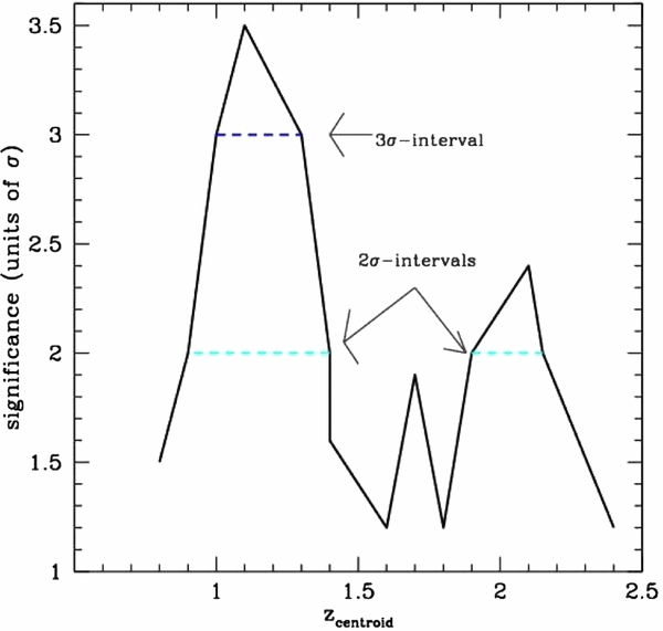
Figure 13. Visual representation of the peak finding algorithm. The centroid of the redshift bin Δz ≃ 0.28 is plotted in the x-axis. The values of  in units of σ are reported in the y-axis. Solid black line: significance as a function of the centroid redshift zcentroid. Horizontal dashed lines: 2σ and 3σ intervals. According to the peak finding procedure, the 2σ interval in the plot associated with the peak at zcentroid ∼ 1.1 is rejected, since it contains entirely the higher significance 3σ interval shown in the figure. No s interval is associated with the peak at zcentroid ∼ 1.7. This is because its significance is less than the 2σ threshold.
Download figure:
Standard image High-resolution imageA.7. Cluster Candidates Selection
The significance s of a given s interval is interpreted as the detection significance of the corresponding cluster candidate. In this section we describe our procedure that provides (1) an estimate for the redshift of the overdensity, (2) an estimate for the cluster core size, and (3) a rough estimate for the cluster richness.
We estimate the size of each cluster candidate in terms of the minimum and maximum distances from the beacon (in our case the FR I) at which the overdensity is detected. According to our procedure, the points of the s interval are associated with different values of  and
and  . We estimate a minimum and a maximum projected radius of the overdensity as the average (and the median) of the minimum (
 ) and maximum distances (
 ) associated with all of the points of the s interval, respectively. The uncertainty is estimated with the rms dispersion around the average. The maximum projected radius also provides an estimate for the cluster core size, as further tested in this work and in Paper II.
In Figure 14 we show the PPM plots of source 01, (after having applied the Gaussian filter) where the radial information concerning rmin (left panel) and rmax (right panel) is considered. Analogously to what was done for Figure 12, we only plot points that are associated with ⩾2σ overdensities (see the legend in the panels for the color code adopted). The vertical solid line in each panel is located at the redshift of source 01. The values of  and
and  associated with the high significance patterns of our plots are very stable with respect to Δz (see Figure 14). Therefore, the particular choice Δz = 0.28 does not affect the results concerning the projected space analysis.
Figure 14. PPM plots for source 01, ⩾2σ points are plotted. Radial cluster information concerning rmin (left panel) and rmax (right panel). See the legend in the panels for information about the color code adopted. In each panel the abscissa of the vertical solid line is at the spectroscopic redshift of the source.
Download figure:
Standard image High-resolution imageWe also estimate the redshift of the cluster as the middle point of the s interval. To estimate the fiducial uncertainty of the cluster redshift we consider all sources located within the median value of the minimum distance and the median value of the maximum distance from the coordinates of the FR I beacon within which the overdensity is detected in the projected space. We also limit to the sources that have photometric redshifts within a redshift bin Δz = 0.28 centered at the estimated cluster redshift. This is done consistently with our detection procedure. The cluster richness is roughly estimated by the number of selected sources. Then, the cluster redshift is estimated at the 1σ level by the rms dispersion around the average of the redshifts of the selected sources.
In particular, if N ≫ 1 sources were uniformly distributed within the redshift bin Δz = 0.28 we would obtain an rms dispersion of 0.08. We expect the estimated redshift uncertainty to be around this value.
A.8. Cluster Candidate—FR I Association
The method described here detects megaparsec-scale overdensities within the entire redshift range spanned by the zcentroid values. Then, we associate with the radio galaxy only those overdensities that are detected in the field, at a redshift compatible with that of the source, i.e., when the interval centered at the redshift estimated for the overdensity and with a half-width equal to two times the fiducial redshift error intersects the redshift range defined within the radio galaxy redshift uncertainties. Multiple overdensity associations are not excluded.
A.9. Considerations about the Redshift Information
We point out that the redshift of the FR I beacon is considered only during the last step of the procedure, when we perform the association between the detected overdensities and the radio galaxy. This is primarily motivated by the fact that we do not have spectroscopic information for most of our FR Is. Therefore, our approach is necessarily different from previous studies which select cluster members using photometric redshifts for the majority of the galaxies in the field, but also knowing the spectroscopic redshifts of some of the cluster members (e.g., Papovich et al. 2010).
Furthermore, our choice implies that the high significance patterns in our plots (see, e.g., Figure 12) have a typical width along the zcentroid axis comparable to the statistical photometric redshift uncertainty σz ∼ 0.054(1 + zcentroid). Such an uncertainty corresponds to sources with i+ ∼ 24 and 1.5 < z < 3 sources (see Table 3 of Ilbert et al. 2009), which we expect to find in our clusters. Therefore, our method estimates the cluster redshifts with similar accuracy. On the other hand, including the (photometric) redshift information of the FR I beacon from the beginning of our procedure would imply an increase of the intrinsic scatter due to the FR I redshift uncertainty. If we sum in quadrature the redshift uncertainty associated with each FR I to the statistical photometric redshift uncertainty σz ∼ 0.1–0.2, the uncertainty increases up to ∼0.2–0.5, depending on the redshift of the radio galaxy and its uncertainty. This effect would make our method ineffective to search for high-z cluster candidates around radio galaxies.
A.10. Generalization to other Data Sets
In this section we describe how the PPM can be generalized for application to other data sets and photometric redshift catalogs, whose statistical redshift accuracy is possibly comparable to or better than that of the Ilbert et al. (2009) catalog. Surveys with depth similar to or higher than that of COSMOS are preferred. In particular, the PPM might be applied to both present and future wide field surveys such as SDSS Stripe 82, LSST, and Euclid.
The parameters should be adapted to take into account the different mean field number density of galaxies in the survey and the statistical photometric redshift uncertainties of the redshift catalog. Therefore, it is not straightforward to provide precise rules.
In general, the redshift bin Δz at which the overdensities are evaluated in the PPM plots should be set equal to the 2σ statistical photometric redshift uncertainty of the galaxies at the redshifts of our interest and magnitudes typical of the sources we expect to find in clusters at high redshifts.
Consequently, the length of the s intervals should be at least about one-third of the specific redshift bin Δz adopted to select the overdensities in the PPM plots. We remind readers that the s intervals are the high significance intervals in the PPM plots (at the specific Δz) that are associated with overdense regions. Similarly, the Gaussian dispersion σw used to remove the noise from the PPM plots should be equal to one-fifth of the abovementioned minimum length for the s interval. As described and motivated in the procedure description (see Section A.6), when defining the s intervals, consecutive intervals that are separated by an amount σw (=0.02 in this paper) or less along the zcentroid axis should be always merged. Such scaling relations are motivated by the fact that the adopted parameters should ultimately rescale linearly with the typical statistical photometric redshift accuracy.
Furthermore, according to the procedure description, we do not change the PPM tessellation with increasing cluster redshift. This is mainly because we are looking for overdense regions with sizes typical of those of the cluster cores and the angular distance DA(z) at the redshift z is fairly constant between z ∼ 1–2. However, it might be appropriate to rescale linearly the size of the PPM tessellation by a factor of ∼DA(z = 1.5)/DA(z) in the case where the PPM is used to search for diffuse protoclusters at redshifts significantly higher than z ∼ 1–2 (e.g., at z ≃ 8, Trenti et al. 2012). This leads to a correction ∼21%, 46%, and 51% at redshifts z ∼ 4, z ∼ 6, and z ∼ 8, respectively.
Footnotes
- 8
We test if cosmic variance affects our analysis by selecting four disjoint quadrants in the COSMOS survey to estimate the field density separately from each quadrant. We verify that the results are independent of the particular choice of the field.
- 9
The function h = f*g is the convolution of the function f with the function g.
- 10
Here M500 is the mass enclosed within the radius encompassing the matter density 500 times the critical.
- 11
We denote by "I" the Subaru i+ magnitude and, if absent, the CFHT i' magnitude. We denote by "K" the CFHT K-band magnitude. All these magnitudes are from the I09 catalog, they are in AB system, and they are measured within an aperture of 3 arcsec diameter.
- 12
The Skellam distribution is the discrete probability distribution of the difference of two statistically independent random variables each having Poisson distributions. In this case, the Skellam probability is chosen because we subtract the cluster members from the field.
- 13
Here r500 (r200) is the radius at which the enclosed mass encompasses the matter density 500 (200) times the critical. In estimating r200 for both F062 and F126 we also assume hydrostatic equilibrium. We use Equation (3) of Reiprich & Böhringer (1999) and the core radius estimates as in Equation (4) of FGH07.
- 14
Here M200 is the mass enclosed within the radius encompassing the matter density 200 times the critical.
- 15
We add the cluster members into each ECF by applying a rigid rotation to all the projected coordinates of the cluster members.
- 16
In fact,
is also a functional of the galaxy number count function at zcentroid and Δz. - 17
Let f and g be two functions defined on some subset of real numbers. f(x) = o(g(x)) as x → x0 if and only if for all K > 0 there exists δ > 0 such that |f(x)| ⩽ K|g(x)|, for each x: |x − x0| < δ.
