


ABSTRACT
Radio scintillation observations have been unable to probe flow speeds in the low corona where the scattering of radio waves is exceedingly strong. Here we estimate outflow speeds continuously from the vicinity of the Sun to the outer corona (heliocentric distances of 1.5–20.5 solar radii) by applying the strong scattering theory to radio scintillations for the first time, using the Akatsuki spacecraft as the radio source. Small, nonzero outflow speeds were observed over a wide latitudinal range in the quiet-Sun low corona, suggesting that the supply of plasma from closed loops to the solar wind occurs over an extended area. The existence of power-law density fluctuations down to the scale of 100 m was suggested, which is indicative of well-developed turbulence which can play a key role in heating the corona. At higher altitudes, a rapid acceleration typical of radial open fields is observed, and the temperatures derived from the speed profile show a distinct maximum in the outer corona. This study opened up a possibility of observing detailed flow structures near the Sun from a vast amount of existing interplanetary scintillation data.
Export citation and abstract BibTeX RIS
1. INTRODUCTION
The solar wind is composed of fast (∼750 km s−1) and slow (∼400 km s−1) speed components. Traditionally, it is thought that the former originates in the open magnetic field regions of coronal holes, while the origin of the latter remains unsettled (Feldman et al. 2005). It was suggested that plasma trapped in closed fields is released by reconnection along the open field lines surrounding the closed field regions (Wang et al. 2000; Woo et al. 2004; Feldman et al. 2005). The analysis of Doppler dimming of line intensities provided outflow speeds of O5+ ions and hydrogen atoms (Strachan et al. 2002; Zangrilli et al. 2002; Teriaca et al. 2003). The derived speeds, however, drop to levels below the detection limit at heliocentric distances of less than 3–4 RS (RS = solar radii) in the quiet-Sun/streamer region. We should also note that the velocity of O5+ can be different from that of the bulk plasma flow by up to ∼50 km s−1 below 5 RS (Ofman 2000). The determination of flow speeds by tracking moving coronal features in time-lapse sequences of coronagraph images has been limited to the streamer stalk region (Sheeley et al. 1997; Wang et al. 2000). To what extent the plasma transport is localized and transient in the quiet Sun region is still unclear.
Here we explore the low and extended corona of the quiet-Sun region by the radio scintillation technique. Solar wind speeds have been measured from radio scintillation spectra using natural radio sources with a small angular diameter (Scott et al. 1983; Tokumaru et al. 1991) and using spacecraft as signal sources (Efimov 1994). The time delay of intensity scintillation between the measurements at two separated radio telescopes also provided estimates of the flow speed (Kojima & Kakinuma 1990; Rickett & Coles 1991; Tokumaru et al. 2012). The applicability of the radio scintillation technique, however, has been limited to heliocentric distances of approximately >5 RS because the excessively strong scattering of radio waves prevents measurements below this height (Tokumaru et al. 1991). Only radar backscatter measurements (James 1966) provided a limited number of flow speed data below this height.
In weak scattering conditions the scintillation spectrum shows a knee feature due to diffraction around the Fresnel frequency, which is proportional to the bulk flow speed perpendicular to the radio ray path (Scott et al. 1983; Tokumaru et al. 1991). This fact enables the determination of the speed once the knee frequency is identified in the observed spectrum. However, this method cannot be used for close distances, where weak scattering breaks down due to the turbulent dense plasma. In such strong scattering conditions the (diffractive) knee frequency deviates from the Fresnel frequency, and an additional bump caused by refractive scintillation is expected to appear at lower frequencies (Rumsey 1975; Gochelashvily & Shishov 1975; Rino 1979; Codona et al. 1986). Because of this complexity, no effort has been made to derive flow speeds from radio scintillation spectra in strong scattering. Although Manoharan (2010) observed a flattening of the power-law spectral feature with decreasing distance and attributed this change to the transition from weak to strong scattering, the limited spectral bandwidth did not allow for the determination of velocity. Narayan et al. (1989) observed fluctuations of the flux from a natural radio source caused by refractive scintillation. The transition from weak scattering to strong scattering occurs around 4 RS for 8 GHz (Tokumaru et al. 1991; Morabito 2007). The transition accompanies the turnover of the scintillation index (e.g., Manoharan 1993).
In this work, we apply for the first time the strong scattering theory to radio scintillation spectra to obtain outflow speeds at 1.5–20.5 RS. Data were obtained using the downlink signal of the Akatsuki spacecraft of Japan (Nakamura et al. 2011), which is on its way to Venus. Coordinated observations were made using the space solar telescope Hinode (Kosugi et al. 2007). Section 2 presents the measurement procedure and the observation conditions, Section 3 presents the scintillation spectrum model, Section 4 presents the observed scintillation spectra, Section 5 derives the flow speeds, Section 6 estimates the temperatures from the flow speeds, Section 7 discusses the nature of turbulence, and Section 8 provides our conclusions.
2. OBSERVATIONS
Observations were conducted on 2011 June 6 to July 8 using the 8.4 GHz downlink signal of the Japanese Venus explorer Akatsuki during solar conjunction. The 16 experiments, each of which has a duration of 4.7–7.5 hr, covered heliocentric distances of 1.5–20.5 RS (Figure 1(a)). The former half of the period (June 6–25) covers the western side of the Sun, and the latter half (June 26–July 8) covers the eastern side. The heliolatitude of the point of closest approach to the Sun (tangential point) changed from 3°N to 77°N on the western side and from 67°N to 10°N on the eastern side. The distance between the spacecraft and the point of closest approach was ∼1.0 × 10⁸ km, and the distance between the point of closest approach and the Earth was ∼1.5 × 10⁸ km. Simultaneous observations using the solar telescope Hinode were conducted during June 24–27 around the period of the minimum heliocentric distance, as Hinode Operation Plan (HOP) 189.

Figure 1. Observation geometry and Sun's condition. (a) Locations of Akatsuki relative to the Sun as seen from the Earth. The Y axis is directed to the north of the Sun. (b) Hinode XRT images, on which the locations of Akatsuki during coordinated observations are plotted. (c) Potential magnetic field on June 25 obtained from a magnetic field map acquired by SOLIS. Black and white shades on the solar surface indicate positive and negative radial magnetic field, respectively. Red and blue curves show away (Br > 0) and toward (Br < 0) open field lines, respectively. Yellow and light blue lines show closed field lines with positive and negative magnetic polarities, respectively. The displayed field corresponds to the dotted square in (a).
Download figure:
Standard image High-resolution imageThe solar activity was in a rising phase in 2011. The X-ray Telescope (XRT) on board Hinode (Golub et al. 2007) did not detect prominent polar coronal holes, except for a small coronal hole in the northeast area (Figure 1(b)). X-ray jets were not observed. The potential magnetic field (Figure 1(c)), which was obtained using the method of Shiota et al. (2012) from a synoptic magnetic field map acquired by Synoptic Optical Long-term Investigations of the Sun (SOLIS; Balasubramaniam & Pevtsov 2011), suggests that closed fields were predominant below the points of closest approach and that quasi-radial field lines originating from the small coronal hole were present around the points of closest approach of the June 25 (1.5 RS) and 26 (1.7 RS) observations. The solar wind synoptic map generated with IPS measurements using natural radio sources at 327 MHz by the Solar-Terrestrial Environment Laboratory of Nagoya University (Kojima & Kakinuma 1990) indicates that slow winds were predominant at the observed latitudes and longitudes (Figure 2): the velocities scatter mostly in the range 400–600 km s−1. The measurement at 12.7 RS (June 13) was influenced by a coronal mass ejection (CME).
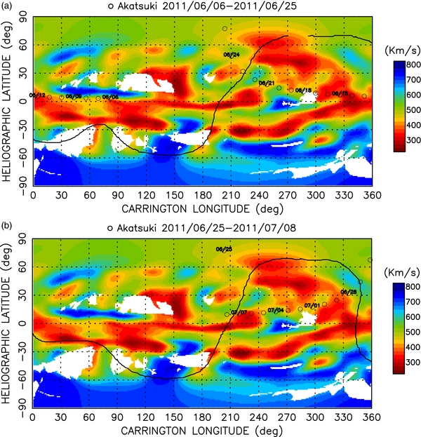
Figure 2. Solar wind velocity synoptic map generated with IPS measurements by the Solar-Terrestrial Environment Laboratory of Nagoya University. The Carrington rotation numbers are (a) 2110 for June 6–25 and (b) 2111 for June 6–July 8. Circles indicate the radial projections of the points of closest approach. Numerals indicate observation dates. The longitudinal shift during propagation was not considered because the distance to the Sun was small and the influence of the solar magnetic field is strong in this region.
Download figure:
Standard image High-resolution imageThe measurements utilized the radio science subsystem of the Akatsuki spacecraft (Imamura et al. 2011). The experiments were conducted using the 8.4 GHz (3.6 cm) downlink stabilized by an on board ultra-stable oscillator (USO) having an Allan deviation less than 10−12 at the integration time 1–1000 s. The radio wave transmitted from the high-gain antenna on the spacecraft is received by the 64 m dish antenna at Usuda Deep Space Center (UDSC) of Japan. The signals received were down-converted to around 125 kHz by an open-loop heterodyne system stabilized by a hydrogen maser and 8 bits digitized with a sampling rate of 500 kHz using a recorder developed for radio astronomy. The amplitude time series retrieved from the open-loop data are used for computing scintillation spectra. Frequency time series are also retrieved from the same data set: the signal time series is divided into successive 1 s blocks, and then the frequency time series is obtained by finding peak frequencies in the fast Fourier transform (FFT) spectra of these blocks.
The magnitude of scintillation is represented by the scintillation index 〈δI2〉/〈I〉2, where δI is the fluctuation in intensity about its mean 〈I〉. Figure 3 shows the scintillation index as a function of the heliocentric distance. The index increases as the distance decreases and reaches values near unity at <5 RS, suggesting that the scintillation is in a strong scattering regime in this region.

Figure 3. Scintillation index as a function of the heliocentric distance on the western side (filled circles) and the eastern side (open circles) of the Sun. The observation at 12.7 RS indicated by an arrow is influenced by a coronal mass ejection (CME). Double-knee spectra typical of strong scattering were observed in the four measurements inside 3 RS.
Download figure:
Standard image High-resolution image3. SCINTILLATION MODEL
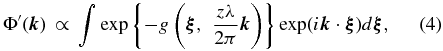
The radio wave is scattered during its passage through the turbulent corona producing a diffraction pattern at the Earth. Because of the rapid increase in the plasma density with decreasing the distance to the Sun, the effect of the medium on the signal phase is represented by a thin phase modulator (phase screen) that is located at the point of closest approach to the Sun. The diffraction pattern at the Earth is convected past the observer at the solar wind velocity and is observed as intensity scintillations. Let kx be the wavenumber in the radial direction defined at the point of closest approach, f the temporal frequency of intensity fluctuation, and V the flow velocity perpendicular to the ray path. The one-dimensional spatial spectrum of intensity at the receiver, ΦS(kx), and the temporal scintillation spectrum, ΦT(f), are related to each other by (Scott et al. 1983)
with f = V kx/2π. Least-squares fitting of a model spectrum to observed scintillation spectra is widely used to find V and other parameters such as the asymmetry factor (Scott et al. 1983; Manoharan & Ananthakrishnan 1990; Tokumaru et al. 1991; Yamauchi et al. 1998). In the present study, however, such a conventional method is not used because of the long computational time needed in strong scattering. Instead, because ΦT and ΦS have a common spectral shape, the velocity can be obtained by finding characteristic spectral features in the observed ΦT and the modeled ΦS and comparing the corresponding characteristic frequency fchar and the characteristic wavenumber kchar:
For the spatial spectrum of the phase modulation, we chose a power-law form with respect to the spatial wavenumber k as k−α, where the exponent α can vary slowly with the solar elongation. This model is consistent with direct plasma observations at greater distances (Marsch & Tu 1990) and radio occultation measurements of phase and intensity fluctuations (Woo & Armstrong 1979; Coles & Harmon 1978; Harmon & Coles 1989; Imamura et al. 2005). The exponent is α = 11/3 for the Kolmogorov turbulent spectrum. The influence of the anisotropy of density irregularities, which is not considered here, will be discussed later. Then, in the case of weak scattering, the second-order statistics of intensity shows that the two-dimensional spatial spectrum of the intensity at the receiver is represented by (Scott et al. 1983; Yakolev 2002)
where  , kx is the wavenumber in the radial direction defined at the point of closest approach, ky is the wavenumber in the direction perpendicular to the radial direction and the ray path,
  ,
,  is the Fresnel wavenumber, λ is the wavelength of the radio wave, and z = L1L2/(L1 + L2) where L1 is the distance between the point of closest approach and the radio source and L2 is the distance between the point of closest approach and the receiver. The
  term is the Fresnel propagation filter. The spherical wave effect is taken into account by using the relation z = L1L2/(L1 + L2) instead of z = L2, which is appropriate for a plane wave (Yakolev 2002; Rino 2011).
Here we consider a more general case including both weak and strong scattering. Considering the propagation of the fourth statistical moment of the electric field, the two-dimensional intensity spectrum is given by (Rino 1979, 2011)
where

D is the phase structure function and  and
and  are spatial vectors. We again assume a power-law spectrum for the phase modulation like k−α. In this case,
  is given by the following formula (Rumsey 1975; Rino 1979, 2011):
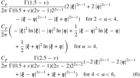
where 2ν + 1 = α, and the parameter Cp is proportional to the power of the electron density fluctuation. The integration (4) is computed similarly to the method of Marians (1975). By using radial symmetry to take  , we obtain
where x = ξx/ξmax, n = kxξmax/2π, and ξmax are taken to be sufficiently large. The integration for x, which is an integration of a highly oscillatory function, is first computed using the algorithm based on Gaussian quadrature formulas developed by Piessens & Haegemans (1974). The integration for ξy is done next in a logarithmic coordinate.
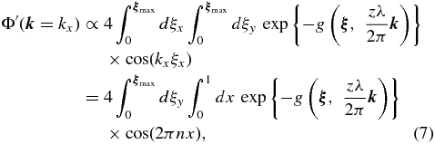
In order to compare the model spectrum with experimental data, the two-dimensional spatial spectrum (4) is integrated to obtain the one-dimensional spatial spectrum:
Figure 4 shows examples of the computed one-dimensional spectra ΦS(kx) for α = 11/3 (Kolmogorov) in the observation geometry. In weak scattering (small Cp), ΦS(kx) is characterized by a single knee caused by diffraction at the wavenumber kdiff, which is close to the Fresnel wavenumber kFresnel, with a power-law dependence  at higher wavenumbers. The use of relation (3) for weak scattering instead of relation (4) yields almost the same spectrum. Since kFresnel is determined only by the observation geometry, kdiff is adopted as the characteristic wavenumber kchar. In strong scattering (large Cp), on the other hand, the spectrum exhibits double knees with a plateau between these. The knee on the high wavenumber side (kdiff) is caused by diffraction, while the inverted knee (kref) beside the bump near the low-wavenumber end is caused by refraction. An increase of the scattering strength shifts kdiff to higher wavenumbers and kref to lower wavenumbers. A physically intuitive understanding of this behavior is presented by Rickett (1990): a stronger phase modulation at the observing plane decreases the field coherence scale (diffractive scale), across which there is a 1 radian difference in the phase modulation; a stronger phase modulation at the same time leads to a larger effective scattering angle, thereby increasing the transverse scale of the scattering disk (refractive scale) influencing the signal arriving at the observing point. Theories suggest that the root of the product,
  , is close to kFresnel (Rumsey 1975; Rickett 1990); our new method adopts this wavenumber as kchar. To summarize,

Figure 4. Model spatial scintillation spectra ΦS(kx) calculated using the formula by Rino (1979). The Cp is proportional to the power of the electron density fluctuation. The power-law index of the phase modulation spectrum is taken to be α = 11/3 (Kolmogorov), and other parameters are the same as those in the observations. The arrow indicates the Fresnel wavenumber kFresnel = 7.5 × 10⁻⁵ rad m−1. Dotted thin lines show examples of finding kchar in a single-knee case (Cp = 10−7) and a double-knee case (Cp = 10−4). The kchar for single- and double-knee spectra are determined by kchar = kdiff and  , respectively.
Download figure:
Standard image High-resolution imageThe corresponding frequencies in temporal scintillation spectra are similarly defined:
4. OBSERVED SPECTRA
Scintillation spectra are obtained using an FFT routine with a Welch window from the intensity time series normalized by the mean intensity. The spectra flatten into a white noise floor near the high-frequency end, while they merge into a common background noise with a negative spectral slope near the low-frequency end. A spectrum almost free from the solar influence, taken in 2011 February when the heliocentric distance was 155 RS, is dominated by these noise components, although the noise levels are not the same as the current observations due to the difference in the observation condition (not shown here). The former noise was removed by subtracting the mean spectral density near the high-frequency end from the entire spectrum. The latter was removed by fitting a linear combination of two power-law functions to the low-frequency portion of the June 6 spectrum, which probed 20.5 RS, and subtracting the fitted function from all of the spectra.
Figure 5 shows the scintillation spectra after removing the noise components mentioned above and smoothing out small-scale structures. The spectra clearly show the expected transition from weak to strong scattering as the distance to the Sun decreases both on the western and eastern sides. At >3 RS, each spectrum shows a single knee, and the scintillation power increases with decreasing distance. At closer distances, each spectrum shows a diffraction knee on the high-frequency side and an inverted refraction knee on the low-frequency side, and the level of the plateau between these decreases with decreasing distance. The spectra at >12 RS show a small bump around 0.01–0.03 Hz; this feature is attributed to a remaining background noise because it disappears as the plateau level increases at closer distances. This is the first observation that clearly identifies refractive scintillation and diffractive scintillation simultaneously.
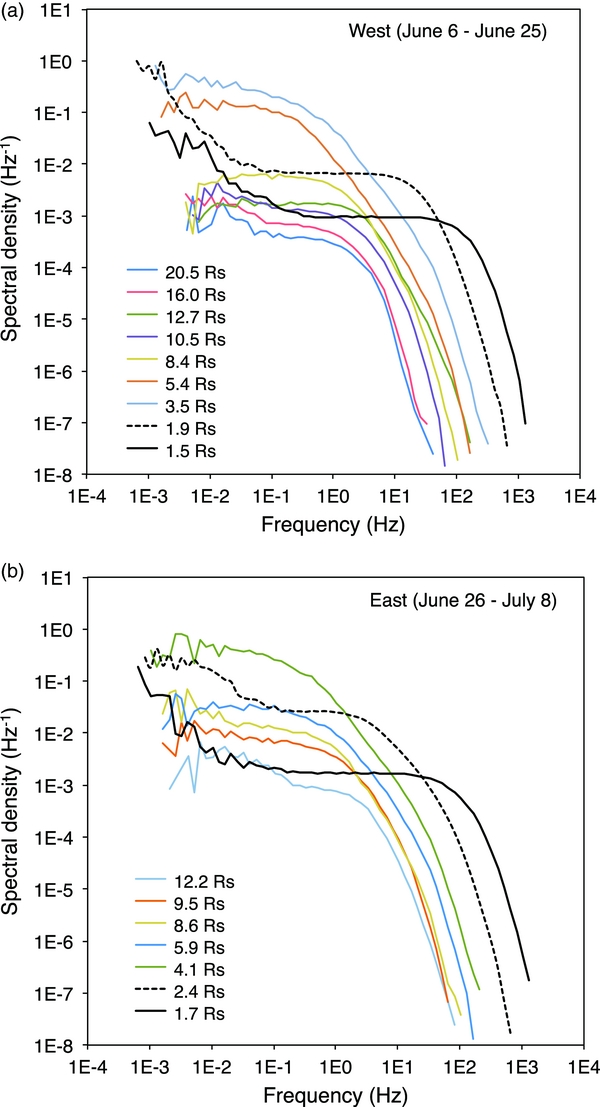
Figure 5. Observed temporal scintillation spectra ΦT(f) on the (a) western and (b) eastern side of the Sun.
Download figure:
Standard image High-resolution imageThe scintillation theory relies on power-law statistics of the phase modulation. The logarithmic spectral slope on the high-frequency side of the diffraction knee represents −α. Although the magnitude of the slope tends to increase with frequency probably due to the effect of the turbulent inner scale, typical values are found to be α = 3–4 at >1 Hz. The α at lower frequencies (0.0003–0.1 Hz) can be estimated from the power spectra of the signal phase measured at the single station. The phase fluctuation is proportional to the fluctuation of the electron density integrated along the ray path, and it is sensitive to plasma irregularities larger than the Fresnel diffraction scale. The phase spectra Φphase(f) shown in Figure 6 were obtained from the signal frequency spectra Φfreq(f) using the relationship Φphase(f) = Φfreq(f)/(2πf)2 (e.g., Efimov et al. 2010). The spectral slope of a phase spectrum represents −(α − 1). Then, although the slope is variable, its magnitude is typically α−1 = 2–3, which means α = 3–4. Model spectra are calculated based on this α.
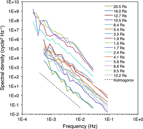
Figure 6. Power spectra of the signal phase observed at the single station. Legends indicating heliocentric distances are listed by dates. The dashed line shows a power law with the index α−1 = 8/3 (Kolmogorov). The frequency ranges dominated by the background noise were removed.
Download figure:
Standard image High-resolution image5. DERIVATION OF FLOW SPEEDS
The analysis method relies on a theoretical expectation that kchar is insensitive to the flow properties. Figure 7 shows the sensitivity of kchar to the power-law exponent α and the density fluctuation parameter Cp. In weak scattering, kchar (=kdiff) is determined by finding the intersection of linear functions fitted to the near straight-line portions of the logarithmic spectrum on the low- and high-frequency sides of the diffraction knee; an example of fitting straight lines to the model spectrum is given in Figure 4. The obtained kchar is always around 6.9 × 10⁻⁵ rad m−1, which is close to the Fresnel wavenumber of kFresnel = 7.5 × 10⁻⁵ rad m−1, with a variability of ±15%; we adopt this kchar in later analysis. In strong scattering, we first find the diffraction knee wavenumber kdiff and the refraction knee wavenumber kref in a similar manner, and then determine the characteristic wavenumber from  (Figure 4). The scintillation theory predicts that kdiff and kref change with scattering strength in such a way that
  is almost unchanged (Section 3). The kchar obtained is always around 1.2 × 10⁻⁴ rad m−1, which is 1.6 times the kFresnel, with a variability of ±7%; we adopt this kchar in a later analysis. The uncertainties in kchar are taken into account in the error estimation.
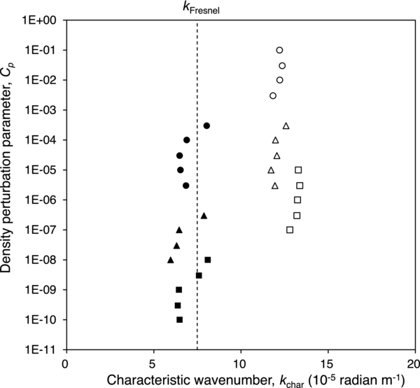
Figure 7. Characteristic wavenumbers kchar determined from model spectra for different values of the scattering strength parameter Cp and the power-law exponent α (circles for α = 3, triangles for α = 11/3, rectangles for α = 4). Filled symbols are for weak scattering having a single knee in each spectrum, while open symbols are for strong scattering having two knees in each spectrum. Intermediate cases, where two knees are located close to each other and linear line fitting is difficult, are excluded from the analysis. The dashed line represents the Fresnel wavenumber.
Download figure:
Standard image High-resolution imageThe characteristic frequency fchar is determined in the same way as kchar (Figure 8). The four spectra at <3 RS are analyzed as double-knee cases, and the remaining spectra are analyzed as single-knee cases. The obtained fchar contains uncertainties because the choice of the fitting interval in the observed spectrum for finding the intersection is rather arbitrary. Based on a visual inspection, the frequencies of both ends of each fitting interval can be reasonably chosen within a factor of two. Then, we consider the changes of the ends of each fitting interval by a factor of  or
or  from the nominal frequencies, and the maximum and minimum speeds among the solutions of all combinations of the fitting intervals determine the error range. This error is also considered in the error estimation.
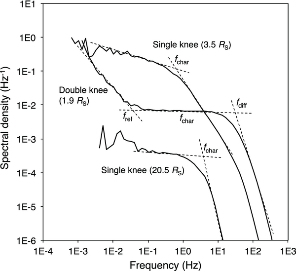
Figure 8. Examples of finding the characteristic frequency. Two single-knee cases and one double-knee case are shown. Linear functions are fitted to both sides of each knee in the logarithmic coordinate, and an intersection is found. The fchar for single- and double-knee spectra are determined by fchar = fdiff and  , respectively.
Download figure:
Standard image High-resolution imageOnce fchar and kchar are determined, the flow speed is obtained by using Equation (2). The rate of change in the heliocentric distance of the radio ray path, whose magnitude is 1–10 km s−1 depending on the observation day, is added to the derived flow speed assuming that the flow direction is radially outward. Figure 9 shows the obtained flow speeds plotted against the heliocentric distance. The speed profiles on the western side and the eastern side are similar. The velocity remains small (<100 km s−1) inside ∼5 RS, increases rapidly with distance at 6–13 RS, and seems to asymptotically approach 400–500 km s−1 at farther distances, being consistent with the IPS measurements (Figure 2). The speeds derived from the single-knee spectra and those from the double-knee spectra are smoothly connected without notable discontinuity, suggesting that the new method successfully derives flow speeds in strong scattering. The absence of notable acceleration at <5 RS is attributed to the influence of closed field lines which were predominant near the Sun (Figure 1(c)).
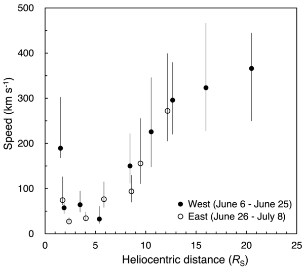
Figure 9. Derived outflow speeds on the western side (filled circles) and the eastern side (open circles) of the Sun, with vertical bars indicating the error range. The error bars do not include contributions from anisotropy of irregularities and random velocity components mentioned in Section 5.
Download figure:
Standard image High-resolution imageSmall, nonzero speeds were steadily observed at <5 RS while the point of closest approach moved over a wide latitudinal range of ∼150° centered at the north pole. This suggests that the supply of plasma to the slow solar wind occurs continuously over an extended area in this height region. This might imply plasma transport along ubiquitous small-scale open field lines that permeate the inner corona (Woo et al. 2004). It should be noted that these nonzero velocities cannot be explained by the velocity dispersion of random turbulent motions because a superposition of various velocity components with the contribution decreasing with velocity would smooth out the double-knee feature in strong scattering.
The rather large speeds of 190 km s−1 at 1.5 RS and 75 km s−1 at 1.7 RS will be attributed to acceleration occurring in open field lines that originate in the small coronal hole near the north pole (Figure 1(c)). Optical measurements and solar wind models suggest that acceleration of up to 100–200 km s−1 at 1.5–1.7 RS is possible above coronal holes (Zangrilli et al. 2002; Teriaca et al. 2003; Suzuki & Inutsuka 2005; Cranmer et al. 2007). Tokumaru et al. (1991) observed similar transient large velocities near the north pole in IPS measurements without notable correlation with coronal holes and suggested possible relationship with CMEs.
The anisotropy of density irregularities, whose major axis is considered field aligned, changes the spectral shape and can influence the velocity determination. The axial ratio of density fluctuations is near unity at >30 RS and increases with decreasing distance inside 30 RS to reach ∼1.5 at 10 RS (Yamauchi et al. 1998) and ∼14 at 2.2 RS (Armstrong et al. 1990). Scott et al. (1983) presented model spectra in weak scattering for axial ratios of 1.0–1.9 and suggested that the primary effect of anisotropy is to round the knee and narrow the power spectrum. Applying our method of finding the diffraction knee to these model spectra, we found that the knee frequency might be underestimated by <20% relative to the isotropic case if the anisotropy in the weak scattering region is within this range. The influence of anisotropy in strong scattering has never been studied. In strong scattering, the spatial scale of irregularities in a certain direction contributing to diffraction is determined by the direction-dependent field coherence scale, which decreases with increasing scattering strength (Section 3). The decrease of the coherence scale diminishes the contribution to diffractive scintillation; this nature will mitigate the influence of anisotropy to some extent. A quantitative estimate, including the influence on the refractive scintillation, is left for future studies.
The random velocity component can also influence the result. Scott et al. (1983) presented model spectra in weak scattering for fractional random velocities of 0.005–0.7 and suggested that the random velocity component also rounds the knee. Applying our method of finding the diffraction knee to these model spectra, we found that the knee frequency might be overestimated by up to ∼30% relative to the zero random velocity case. The influence in strong scattering will be qualitatively similar.
6. TEMPERATURE PROFILE
Sheeley et al. (1997) showed that feature-tracked speeds above streamer cusps cluster around a nearly parabolic path characterized by a constant acceleration of ∼4 m s−2, and that the acceleration is consistent with the Parker's solution of the solar wind at a temperature of ∼106 K. We apply their method to the speed profile obtained in this study to examine the consistency with thermal expansion. Assuming a steady-state radial flow, the momentum equation, the continuity equation, and the equation of state are combined to have
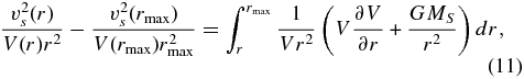
where  is the sound speed, where kB, T, and mp are the Boltzmann constant, the temperature and the proton mass, respectively, r is the heliocentric distance, V(r) is the observed velocity profile, G is the gravitational constant, MS is the solar mass, and rmax is an arbitrary upper boundary. The rmax is taken to be sufficiently distant (100 RS) so that the second term on the left hand side is negligible (∼1%) as compared to the first term.
The V(r) must be a continuous function of r. Under a constant radial acceleration a, it is given by

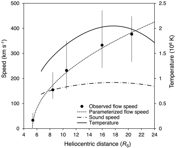
where r0 is a distance where the speed would vanish if the profile is extrapolated to this point. Fitting function (12) to the observed speeds at >5 RS on the western side, we obtain a = 6.6 m s−2 and r0 = 5.3 RS, and the fitted function seems to well approximate the observed speeds (Figure 10). The measurement at 12.7 RS (June 13) was influenced by a CME, and thus it is not used in the analysis. The modeled constant acceleration profile is connected at 24 RS to another smooth function that asymptotically approaches 500 km s−1 to be consistent with the IPS measurements. The solutions of vs and T include a sudden rise around r0 where the modeled velocity vanishes; since the steady state assumption breaks down at this height, the sudden rise is considered spurious (Sheeley et al. 1997), and thus the calculated values in this region are excluded.
Figure 10. Estimation of temperatures from the observed speed profile. Observed flow speeds on the western side at >5 RS (dots), constant-acceleration profile fitted to the observations (dotted), derived sound speed profile (dot-dashed), and derived temperature profile (solid).
Download figure:
Standard image High-resolution image
The derived temperatures of 1–2 × 10⁶ K (Figure 10) are consistent with optical measurements (Strachan et al. 2002; Zangrilli et al. 2002; Teriaca et al. 2003), suggesting that the speed profile in this height region is well explained by radial acceleration in open fields. The sonic point exists around 7.5 RS. The occurrence of the temperature maximum around 18 RS will reflect energy deposition at closer distances by turbulence and compressive waves induced by Alfvén waves (Suzuki & Inutsuka 2005; Cranmer et al. 2007). Alfvén waves will be generated by nanoflares as well as by convection-driven jostling of magnetic flux tubes in the photosphere (Isobe et al. 2008).
7. TURBULENCE
Spectral broadening observations using radars and spacecraft have shown that power-law density fluctuations extend to scales as small as 0.1–1 km at 2.2 RS (Woo & Armstrong 1979; Harmon & Coles 1989). In the present analysis, the combination of the scintillation spectra (Figure 5) and the phase spectra (Figure 6) suggests existence of roughly power-law density fluctuations spanning 6 orders at heights down to 1.5 RS. Based on the derived speeds, the frequency range corresponds to wavelengths from 105 km to 100 m. The smallest scale of 100 m is still larger than the proton gyroradius of ∼30 m in this region, which is calculated from the potential magnetic field (Figure 1(c)) and a temperature of ∼106 K. The shift of the diffraction knee to higher wavenumbers in strong scattering enables sounding of such small scales. The sounding of scales as large as 105 km is made possible by refractive scintillation. The suggested power-law density spectrum implies well-developed turbulence presumably generated by Alfvén waves (Cranmer et al. 2007). Nanoflares distributed over a wide scale range (Aschwanden & Parnell 2002) might also play a role. These processes should be closely related to coronal heating.
We should also note that the logarithmic interval of the plateau between the two knees is almost unchanged from 1.9 RS to 1.5 RS on the western side (Figure 5(a)). This suggests that the open field lines, which affected the observation at 1.5 RS, had weaker turbulence than surrounding closed field lines. This is consistent with the decrease of the density fluctuation above the coronal hole region reported by Manoharan (1993) and Coles (1995). The decrease of the plateau level at 1.5 RS is attributed to the larger speed in this region because of relationship (1).
8. CONCLUSIONS
The coronal continuous outflow in the vicinity of the Sun has been studied by applying strong scattering theory to radio scintillation. The double-knee spectral feature typical of strong scattering was clearly seen near the Sun, enabling the determination of the flow speed based on the theoretical expectation that the square root of the product of the two knee frequencies is proportional to the flow speed. The speeds derived from the single-knee spectra and those from the double-knee spectra are smoothly connected without notable discontinuity, suggesting that the new method successfully derives flow speeds in strong scattering.
No notable acceleration was seen at <5 RS probably due to the influence of closed field lines, which were predominant during the observation period. Nevertheless, small, nonzero speeds were steadily observed in this region while the point of closest approach moved over a latitudinal range of ∼150° centered at the north pole. This suggests that the supply of plasma to the slow solar wind occurs continuously over an extended area in this height region. At higher altitudes a rapid acceleration typical of radial open fields is observed, and the temperatures estimated from the speed profile show a distinct maximum around 18 RS. The occurrence of this temperature maximum will reflect energy deposition at closer distances, which might drive the solar wind. The rather fast winds observed at 1.5 RS and 1.7 RS near the north pole are attributed to acceleration occurring in open field lines originated in a polar coronal hole. Power-law density fluctuations down to the scale of ∼100 m were observed at ∼1.5 RS by virtue of the spread of the spectral feature to high wavenumbers in strong scattering. This feature indicates well-developed turbulence, which can play a key role in heating the corona.
It should be noted that propagating waves can influence the measurements. Flow speeds measured by the two-receiver method sometimes suffer from biases caused by Alfvén waves propagating through field-aligned density irregularities (Grall et al. 1996; Harmon & Coles 2005). Observations using solar telescopes suggest ubiquitous outward-propagating Alfvénic motions having periods of 100–500 s (De Pontieu et al. 2007; Tomczyk et al. 2007; McIntosh et al. 2011). Such long-period waves hardly influence the intensity spectra obtained by the single-station method, although contributions of shorter-period waves cannot be ruled out. Furthermore, the observed flow speeds are much smaller than the Alfvén speeds in the corresponding regions, and thus they do not seem to reflect propagation of Alfvén waves. Using the plasma densities measured from the white light polarization brightness obtained by the Mk4 coronagraph at the Mauna Loa Solar Observatory (Elmore et al. 2003) and the potential magnetic field (Figure 1(c)), the Alfvén speeds around the points of closest approach of the June 25 and 26 observations (1.5 and 1.7 RS) are estimated to be 400–600 km s−1. The Alfvén speed in open fields is typically 1000–2000 km s−1 (Sittler & Guhathakurta 1999; Verdini & Velli 2007). Acoustic waves are compressive waves, and thus they can also influence the measurements (Grall et al. 1996). For the typical coronal temperature of 1–2 × 10⁵ K, the sound speed is 130–180 km s−1. Considering that the observed flow speed increases with distance monotonically from subsonic to supersonic, the contribution of acoustic waves should also be minimal.
The merit of the radio scintillation technique is that it can cover a wide heliocentric distance range as compared to other remote sounding methods. It is also possible to observe simultaneously compressible waves by spectral analysis of frequency time series (Efimov et al. 2012); an analysis of such wave features using the same data set is ongoing. Faraday rotation measurements to estimate the magnetic field intensity is also possible (Pätzold et al. 1987; Efimov et al. 2013; Jensen et al. 2013). The information obtained by such radio propagation experiments is complementary to spectroscopic and imaging observations using solar telescopes.
The telecommunication system of any planetary spacecraft can be used for the proposed observation; it is possible to utilize the solar conjunction opportunities of such spacecraft as well. Furthermore, the temporal and spatial coverage would be greatly improved if the method can be applied to IPS measurements using natural radio sources. The double-knee spectral feature typical of strong scattering is frequently observed also in IPS spectra near the Sun obtained at the Kashima Space Research Center of Japan. The proposed technique, when applied to existing vast amount of IPS data, would reveal the temporal and spatial variation of the coronal outflow near the Sun to further constrain the mechanism of solar wind generation.
We thank the members of the Akatsuki project team, VLBI group, and UDSC operation team for supporting the experiment. N. Mochizuki supported operation of the recording system. The ultra-stable oscillator on board the Akatsuki spacecraft was manufactured by TimeTech GmbH. Courtesy of the Mauna Loa Solar Observatory, operated by the High Altitude Observatory, as part of the National Center for Atmospheric Research (NCAR). NCAR is supported by the National Science Foundation of the U.S. We also thank the referee for making constructive comments that enhanced this paper.