


ABSTRACT
Three magnetic cloud events, in which solar impulsive electron events occurred in their outer region, are employed to investigate the difference of path lengths L0eIII traveled by non-relativistic electrons from their release site near the Sun to the observer at 1 AU, where L0eIII = vl × (tl − tIII), vl and tl being the velocity and arrival time of electrons in the lowest energy channel (∼27 keV) of the Wind/3DP/SST sensor, respectively, and tIII being the onset time of type III radio bursts. The deduced L0eIII value ranges from 1.3 to 3.3 AU. Since a negligible interplanetary scattering level can be seen in both L0eIII > 3 AU and ∼1.2 AU events, the difference in L0eIII could be linked to the turbulence geometry (slab or two-dimensional) in the solar wind. By using the Wind/MFI magnetic field data with a time resolution of 92 ms, we examine the turbulence geometry in the dissipation range. In our examination, ∼6 minutes of sampled subintervals are used in order to improve time resolution. We have found that, in the transverse turbulence, the observed slab fraction is increased with an increasing L0eIII value, reaching ∼100% in the L0eIII > 3 AU event. Our observation implies that when only the slab spectral component exists, magnetic flux tubes (magnetic surfaces) are closed and regular for a very long distance along the transport route of particles.
Export citation and abstract BibTeX RIS
1. INTRODUCTION
1.1. Motivation of the Research
Magnetic clouds (MCs) are defined as interplanetary (IP) magnetic flux ropes characterized by smooth rotations of the magnetic field direction of about 180°, enhanced magnetic field strengths, as well as low proton temperatures and plasma β values (Burlaga 1995). They compose about ∼30% of all IP corona mass ejections (Richardson & Cane 2010) and have force-free magnetic field configurations originally connected to the Sun. As shown in Figure 1, where we reproduce a cartoon of MC drawn by Burlaga et al. (1990), the field line in MC is more wound and therefore longer in length, with increasing distance from the flux rope axis.
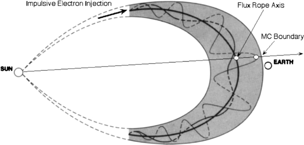
Figure 1. Cartoon of MC at 1 AU, drawn by Burlaga et al. (1990), shows that inside the MC, the field line is more wound and therefore longer in length with increasing distance from the flux rope axis.
Download figure:
Standard image High-resolution imageOccasionally, solar impulsive electron events (Reames 1999) occur within an MC. Since low-energy electrons in the impulsive event could transport scatter freely (Lin 1974), the arriving time of observed non-relativistic electrons can be used to infer the path length traveled by electrons from their injection site near the Sun to the observer, and hence the length of field lines, along which electrons transport. In Figure 1, we see that an observer (open circle) near the flux rope axis could detect particles transporting along a field line that is similar to the Parker spiral line with a length of ∼1.2 AU, while an observer located in the outer region near the MC boundary should detect particles transporting along a highly wound field line having a length of >3 AU according to current MC models (Kahler et al. 2011). However, in the outer region of the MC events surveyed by Kahler et al. (2011), no electron path length of >3.2 AU had been found except for the 1995 October 18–20 MC.
In Tan et al. (2013), we attempted to explain why, in the MC outer region, Kahler et al. (2011) did not observe the electron path length L0eIII > 3.2 AU except for the 1995 October 18–20 MC no. 6, where L0eIII = vl × (tl − tIII), with vl and tl being the velocity and arriving time of electrons in the lowest energy channel (∼27 keV) of the Wind/3DP/SST sensor, respectively, and tIII being the onset time of type III radio bursts (RBs). In addition, the MC number (MC no.) is taken from the "Magnetic Cloud Table 2" in http://wind.nasa.gov/mfi/mag_cloud_S1.html. We noted that, in order to observe L0eIII > 3 AU in the IP medium, electron scattering should be extremely weak. In that sense, MC no. 6 is unusual because of its negligible electron scattering level, which could be seen from the observation of Larson et al. (1997) that, in the event, the deduced path length of electrons is independent of electron energy, Ee.
However, further analysis indicates that our argument described above is insufficient because a negligible electron scattering level may appear in both L0eIII > 3 AU and ∼1.2 AU events. For example, in the 1998 May 2–3 MC no. 32 examined by Torsti et al. (2004) and Tan et al. (2012, 2013), the enhancement of impulsive electron intensities occurred in the MC outer region, where the model-predicted length of magnetic filed lines is >4 AU (see Table 1 in Kahler et al. 2011). In addition, the observed electron path length is Ee independent (see Figure 3 in Tan et al. 2013). Nevertheless, the deduced L0eIII value (see Table 1 in Tan et al. 2013) is only ∼1.2 AU.
Smith et al. (1999) noted that, in MCs, the magnetic fluctuation is more nearly transverse to the mean magnetic field direction than that in the undisturbed solar wind, signifying that the orientation of the wave vector is at a larger angle relative to the mean field. Since such orientation is particularly ineffective at resonantly scattering charged particles, the L0eIII value would be increased with the increase of the two-dimensional (2D) turbulence component. Motivated by Smith et al. (1999), below we examine whether the observed turbulence geometry could affect the L0eIII value.
1.2. Current Status of Turbulence Geometry Study
The one-dimensional ("slab") component of solar wind turbulence, whose wave vector k∥Bm with Bm being the mean vector of the magnetic field B, was first assumed based on the observed fact that the magnetic turbulence could be approximated by Alfvénic fluctuations that are propagated outward from the Sun in high-speed solar wind streams (Belcher & Davis 1971). In the slab model, on a plane perpendicular to Bm, two orthogonal components of δB, where δB is the fluctuation of B, would be symmetric (Matthaeus & Smith 1981). However, because of the presence of the mean magnetic field, the dynamic evolution of magnetic turbulence could lead to an anisotropic quasi-2D turbulence component having k⊥Bm and δB⊥Bm, as first suggested by Matthaeus et al. (1990).
The property of solar wind turbulence depends on the wave frequency, which is denoted by ν0 and ν in the spacecraft frame and plasma frame, respectively. Between ν0 < ∼0.1 Hz, which belongs to the inertial range, and ν0 > ∼0.5 Hz, which could be interpreted as the dissipation range, there exists a frequency ν0b, at which the power law spectral index q for the frequency (ν0) spectrum of the power spectral density (PSD) in magnetic fluctuations (i.e., PSD ∝ ν0−q) shows a sudden increase. However, it should be noted that the precise mechanism that causes the steepening on the spectrum is still under debate. It could be the dissipation of electromagnetic turbulent energy in the solar wind and/or a further small-scale turbulent cascade (Alexandrova et al. 2013).
Bieber et al. (1994, 1996) suggested a composite slab/2D model of solar wind turbulence, in which the energy fraction of the 2D component in the transverse fluctuations reaches ∼85% in the inertial range. Furthermore, in the undisturbed solar wind, Leamon et al. (1998a) extended the examination of turbulence geometry to include the dissipation range, using a database consisting of 35 one-hour intervals of Wind/Magnetic Field Investigation (MFI) interplanetary magnetic field (IMF) data. They found that the fractions of 2D components are ∼89% and ∼54% in the inertial and dissipation ranges, respectively. The decrease of the 2D fraction in the dissipation range could be due to the preferential dissipation of the oblique structure (Leamon et al. 1998a). Also, Hamilton et al. (2008) expanded the database to include 960 intervals of ACE magnetic field data spanning a broad range of solar wind conditions, including MCs. They found that in the undisturbed solar wind, the previous conclusion by Leamon et al. (1998a, 1998b) is upheld. However, in MCs, the slab fractions calculated by using different methods show huge differences.
1.3. Improvement of Time Resolution of Magnetic Turbulence Analysis in the Dissipation Range
Knowledge on the turbulence geometry in the solar wind, especially in MCs, is important for understanding the resonant scattering of charged particles. In the resonant scattering theory, we are restricted to consider the transverse turbulence, ignoring the contribution of the turbulence power component parallel to Bm (P||) (Bieber et al. 1996). Among the turbulence power components perpendicular to Bm (P⊥), only the slab component with its wave vector k∥Bm scatters charged particles, while the 2D component with its wave vector k⊥Bm does not scatter particles. This is because the wave vector of the 2D component is perpendicular to the helical particle orbit. Thus, the power component that resonantly scatters charged particles should be rP⊥, where r is the slab fraction in the transverse fluctuations over the ν0 range relevant to particle scattering. It is noted that resonant scattering of energetic ions with Alfvén waves occurs in the inertial range, where the slab fraction r is only ∼15% in the undisturbed solar wind (Bieber et al. 1996; Leamon et al. 1998a). Therefore, the mean free path of energetic ions predicted by the quasi-linear theory (Jokipii 1966; Hasselmann & Wibberenz 1968), where only the slab model is taken into account, could be less than that deduced from the solar energetic particle (SEP) and cosmic ray observations by one order of magnitude.
To our knowledge, however, there has been no attempt to correlate electron scattering with turbulence geometry. The non-relativistic electrons detected by the Wind/3DP/SST sensor should be resonantly scattered with the R-mode whistler waves at ν0 ∼ 1 Hz (see Tan et al. 2011), which belongs to the dissipation range. Therefore, in order to correlate electron scattering with turbulence geometry, we need to examine the magnetic turbulence in the dissipation range. Since the transport time of non-relativistic electrons from their injection site near the Sun to the 1 AU observer is the order of 1 hr, a time resolution of better than 1 hr should be necessary to carry out such examination.
Also, the database structure recently used in the turbulence geometry analysis may limit the improvement of time resolution. This is because in order to measure PSDs of magnetic turbulences in both the inertial and dissipation ranges, the width Δt of sampled IMF subintervals is usually ⩾1 hr (Leamon et al. 1998a; Smith et al. 2006; Hamilton et al. 2008). While a narrower Δt is enough to sample the dissipation range (ν0 > 0.5 Hz), a wider Δt is necessary in order to sample the inertial range (ν0 < 0.1 Hz). Therefore, a possible approach to diminish the limitation of time resolution is to "untie" the PSD measurements in the two ranges; we will only measure the PSD in the dissipation range.
Here, we choose two main timescales used in the data structure for the analysis of magnetic turbulence in the dissipation range.
- 1.The sampled period Δtm of the local mean magnetic field, which should be the field averaged on a neighboring scale larger than the scale of the fluctuations examined (Alexandrova et al. 2008). Since we only analyze the magnetic turbulence in the dissipation range, the minimum frequency sampled could be ν0mim ∼ 0.1 Hz. With an increasing factor k ∼ 5 of neighboring scales, we have Δtm ∼ k/ν0mim ∼ 1 minute.
- 2.The sampled subinterval width Δt of IMF data with a time resolution of τ0 = 92 ms. It is noted that the variation of the observed slab fraction (r) versus the Δt value (i.e., the sampled data number N per subinterval) in the MC events examined could be used to find a proper value of N(Δt). Since the deduced r value is nearly unchanged between N = 2048 (211) and N = 8192 (213), N = 4096 (212), which corresponds to Δt = Δt0 = 6.28 minutes, should be a proper choice of sampled subinterval width. In fact, a detailed analysis about the width of sampled subintervals is later shown in Section 3.1. We are hence able to accomplish continuous monitoring of turbulence geometry with a time resolution of ∼six minutes.
Here, we assume that Δt is unchanged in the calculation of magnetic turbulence parameters, which results in the presence of a proper Δt value for a given frequency range. However, sophisticated techniques have been developed to analyze turbulence properties over a wide range of frequencies. For example, Sahraoui et al. (2006, 2009) used the k-filtering technique and Alexandrova et al. (2008) used the Morlet wavelet transform to obtain the best estimate of PSDs in a full 4D (ν0, k) space, leading to the possibility of analyzing the ν0 range between (10−3, 103) Hz by only using 1 hr subinterval data. Here, we will not refer to those techniques and keep the data structure with Δtm = 1 minute and Δt0 = 6.28 minutes.
1.4. Questions to be Addressed in This Work
As introduced in Section 1.1, our task is an attempt to explain why, in the highly wound outer region of MCs, a negligible IP scattering level cannot guarantee L0eIII > 3 AU in the solar impulsive electron event. In order to accomplish the task we need to carry out the following work:
- 1.to select MC events in which the impulsive electron event is observed in their outer region and to calculate the L0eIII value by assuming that electron injection occurred at the onset time of type III RBs (Tan et al. 2013);
- 2.to carry out the analysis of turbulence geometry in the dissipation range in order to calculate the slab fraction r in the transverse turbulence;
- 3.to compare the characteristics of transverse turbulences in intervals, where r is calculable, with that in intervals, where r is indeterminate, to verify whether the nature of turbulences could be common in the two kinds of intervals; and
- 4.to analyze the correlation of turbulence characteristics with the ambient solar wind parameters in order to understand the nature of turbulence.
Our investigation on the turbulence geometry in MCs is different from the previous works, such as Hamilton et al. (2008). The database of Hamilton et al. (2008) includes an MC subset comprising 393 intervals from 28 MCs during the years 1998–2002. In their MC subset, all intervals are equally viewed as the MC sample without taking into account their location relative to the MC axis. However, it can be seen from the time profile of the P⊥/P|| ratio, as given by Leamon et al. (1998b) and Smith et al. (1999), that the ratio shows temporal variation inside MCs. Also, Tan et al. (2013) noted that the magnetic fluctuation near the outer boundary of an MC could be different from that in the MC center. Therefore, we will investigate the temporal variation of turbulence geometry detected by a spacecraft when it passed an MC. Through our investigation, we will attempt to answer the following questions.
- 1.Does the slab fraction depend on the distance from the MC axis?
- 2.What is the difference of slab fractions in different MC events?
- 3.Is the slab fraction in MCs correlated with the L0eIII value of solar impulsive electron events?
Observations on the path length of non-relativistic electrons in the impulsive electron event and the slab fraction of magnetic turbulences in the dissipation range are presented in Section 2 and discussed in Section 3. Also, we summarize the main finding in Section 4.
2. OBSERVATIONS
2.1. Selection of Magnetic Cloud Events
In view of the initial feature of this work, it is adequate to carry out a detailed analysis of several typical MC events. When it is possible, we will pick up the MC event with Q0 = 1 in Table 1 of Kahler et al. (2011), indicating a good fit with the MC model. In addition, there must be at least an impulsive electron event that occurred in the outer region of MCs with a >3 AU length of magnetic field lines predicted by MC models (Kahler et al. 2011). Thus, three MC events are chosen for our purpose. These events show typical features of MCs, such as a smooth ∼180° rotation of the magnetic field direction, high field strength, and low plasma β (Burlaga 1995). Basic timing and path length parameters of these impulsive electron events are listed in Table 1.
Table 1. Slab Fraction r of Magnetic Turbulence at ν0 = 1 Hz in the Solar Wind and Path Length L0eIII of Non-relativistic Electrons in Three Magnetic Cloud Events
| MC No. | Year | Start Timea | tIIIb, c | tl at 27 keV | th at 65 keV | End Timea | r | r (P0XX + P0YY) at 1 Hz | L0eIII | LLb | LFCb |
|---|---|---|---|---|---|---|---|---|---|---|---|
| (UT) | (UT) | (UT) | (UT) | (UT) | (nT2 Hz−1) | (AU) | (AU) | (AU) | |||
| 6 | 1995 | Oct 18 19.8 | 19:48 | 21:17.0 | 20:52.8 | Oct 20 01.3 | 0.96 ± 0.04 | ( ) ×10−4 ) ×10−4 |
3.27 ± 0.12 | 2.3–5.1 | 2.0->5 |
| 32 | 1998 | May 02 12.3 | 13:27 | 14:02.1 | 13:52.4 | May 03 17.3 | 0.46 ± 0.31 | (4.3 ± 3.8) × 10 −5 | 1.31 ± 0.05 | >10 | 4.1–7.6 |
| 81 | 2004 | Aug 29 18.7 | 18:01d | 19:16.3d | 19:00.1d | Aug 30 20.8 | 0.80 ± 0.13 | (2.0 ± 1.8) ×10−4 | 2.86 ± 0.17 | 4.1–5.0 | 2.1 |
Notes. The light travel time of 8.3 minutes from the Sun to the Earth is subtracted from the electromagnetic radiation observation time at 1 AU. The sampled time interval in the calculation of r and r (P0XX + P0YY) is between tIII and tIII + 3 hr (see the text). aFrom Magnetic Cloud Table 2 at http://wind.nasa.gov/mfi/mag_cloud_S1.html. bFrom Kahler et al. (2011), where LL and LFC are the field line lengths predicted by the Lundquist model and the flux conservation model, respectively. cFrom Gopalswamy et al. (2012) for MC no. 32. dOn August 30.
Download table as: ASCIITypeset image
In the MC events no. 6 and 32, a strong impulsive electron intensity enhancement was near the front boundary of MCs, whereas the enhancement was near the back boundary in MC no. 81. The electron events are identified from the type III RB data of Wind/WAVES (Bougeret et al. 1995; Kahler et al. 2011; Gopalswamy et al. 2012) and from the electron intensity data of Wind/3DP/SST (Lin et al. 1995).
In order to unify the definition of plasma parameters in the solar wind during the sampled MC intervals, we use the plasma data given by the OMNIWeb (J. King and N. Papitashvili, http://omniweb.gsfc.nasa.gov/html/HROdocum.html). For each MC event, the data of the solar wind speed, Vsw, and the proton number density, Np, are taken from both the Wind/Solar Wind Experiment (see Ogilvie et al. 1995) and OMNIWeb. Comparison is then made between the two data sets in order to determine the delay of OMNI data relative to Wind data. The average delays of 0.7, 0.8, and 1.1 hr are found for MC no. 6, 32, and 81, respectively. Having completed the delay correction, the OMNI data are used to characterize the sampled MC interval.
2.2. Deduction of Electron Path Lengths
Following Tan et al. (2013), the Wind/3DP/SST non-relativistic electron data after the deposition energy loss correction are used in our analysis. By assuming that the onset time tIII of type III RBs as deduced from the Wind/WAVES instrument is the injection time of electrons, from the onset time t of electrons observed at 1 AU we deduce the electron path length LeIII(Ee) = v × (t − tIII), where v is the velocity of electrons at Ee. The LeIII(Ee) value is plotted versus the reciprocal of v in the upper panel of Figure 2, while the ratio of LeIII/L0eIII, where L0eIII is the LeIII value at Ee = 27 keV, is shown in the lower panel of the same figure. It can be seen that the LeIII values in all three MC events are approximately Ee independent, indicating very weak IP scattering of electrons. In addition, from the lower panel of Figure 2, the increasing rates of LeIII/L0eIII versus 1/v are comparable in both MC no. 6 and MC no. 32, in spite of large differences in their L0eIII values. Therefore, Figure 2 is in support of our notion in Section 1.1 that a negligible IP scattering level may appear in the impulsive electron events with very different L0eIII values.

Figure 2. Assuming that the injection time of Wind/3DP/SST electrons is the onset time of type III radio bursts, for the three MC events listed in Table 1, the deduced electron path length LeIII and the ratio of LeIII to L0eIII, the LeIII value at the lowest energy channel (Ee ∼ 27 keV) of the Wind/3DP/SST sensor are plotted vs. 1/v, where v is the electron velocity, in the upper and lower panels, respectively.
Download figure:
Standard image High-resolution image2.3. Deduction of Slab Fractions in the Dissipation Range
2.3.1. Coordinate Systems Relative to the Mean Magnetic Field Direction
We first transform the IMF observation to a coordinate system that is related to the mean magnetic field, Bm. According to Belcher & Davis (1971), the new system has the coordinate axes 1, 2, and 3 corresponding to B0 × R, B0 × (B0 × R), and B0, respectively, where B0 = Bm/|Bm| and R is the radial direction. On the other hand, Bieber et al. (1996) used an equivalent right-handed system that has the coordinate axes x, y, and z corresponding to B0 × (B0 × R), −B0 × R, and B0, respectively. We adopt the terminology of Bieber et al. (1996) because it is based on the standard turbulence nomenclature.
2.3.2. PSD Calculation of Magnetic Fluctuations
From the Wind/MFI magnetic field data with a time resolution of τ0 = 92 ms, we calculate the PSDs of magnetic fluctuations in the dissipation range, using the fast Fourier transformation with a Parzen window included (Tan et al. 2011). Because of the high background of PSDs found in the Wind/MFI data at ν0 > 2.5 Hz (Leamon et al. 1998a; Tan et al. 2011), we limit the sampled ν0 range between 0.67–1.5 Hz in order to calculate the turbulence parameters at ν0 = 1 Hz.
As explained in Section 1.3, we take the sampled subinterval width Δt0 = 6.28 minutes (the sampled data number N = 4096 per subinterval). It is noted that missing data appears in the Wind/MFI archive. However, during nine-day intervals covering the three MC events listed in Table 1, the missing data fraction is only 0.009 ± 0.003 per day. In addition, we calculate the actual width Δt of each sampled subinterval. We find that only <1% of sampled subintervals have Δt − Δt0 > 1 minute. These abnormal subintervals have been removed from further statistical analysis. As a result, in the remaining subintervals, we could ignore the nonlinearity caused by the presence of missing data, assuming that the distribution of data points is even along the time axis.
Having completed the coordinate transformation relative to the mean magnetic field direction, we divide the IMF data into subintervals, each of which has N = 4096. For each subinterval from the deduced PSD data, we carry out the least-squares fit between log(P) and log(ν0), within the ν0 range of 0.67–1.5 Hz, from which the slope (q) and the intercept (P0) at ν0 = 1 Hz are calculated. According to Bieber et al. (1996), the logarithmic average is better than the arithmetic average because it is equivalent to the geometric average, which can avoid the influence of extreme members in the data set.
2.3.3. Calculation of Slab Fraction in MC No. 6
2.3.3.1. PSD data in MC no. 6
As an example, we introduce the slab fraction (r) calculation in the famous 1995 October 18–20 MC no. 6 (Lepping et al. 1997). During a 2.5 day interval covering the MC, the time profiles of P0 and q at ν0 = 1 Hz as deduced from the ν0 range of 0.67–1.5 Hz are shown in the top and second panels of Figure 3, respectively, where the sheath after the shock, MC boundaries, and prominence material as defined by Burlaga et al. (1998) are clearly seen (also see Leamon et al. 1998b). In addition, we define the components of P0 (at ν0 = 1 Hz) along the x, y, and z axes of Bieber et al. (1996) as P0XX, P0YY, and P0ZZ, respectively. It is evident that, inside the MC along the Bm direction, the parallel power (P|| = P0ZZ) is much weaker than the perpendicular (transverse) power (P⊥ = P0XX + P0YY). In addition, the observed qY is often greater than qX, but both qX and qY are greater than qZ. Actually, inside the MC, the mean values of qX and qY are 2.1 and 2.5, respectively, which are greater than the Kolmogorov value (5/3) because the q measurement is carried out in the dissipation range (Leamon et al. 1998a).

Figure 3. For MC no. 6, the time profiles of the PSD component (P) (top panel), spectral index (q) (second panel), ratio of transverse to parallel power (P⊥/P|| = (P0XX + P0YY)/P0ZZ) and the real width Δt of sampled subintervals (third panel), the P0YY/P0XX ratio compared with qY (fourth panel), and the slab fraction r and θBV (bottom panel) are given at ν0 = 1 Hz as deduced from the ν0 range of 0.67–1.5 Hz. In the bottom panel, we show θBV and r by using red and blue lines, respectively. In addition, in view of the large amplitude fluctuation of r, we plot the real value of r by using a light blue thick line and the overall trend of r by using a dark blue line. The light green band is the sampled time interval of impulsive electron events listed in Table 1.
Download figure:
Standard image High-resolution imageFurthermore, the ratio of transverse to parallel power P⊥/P|| = (P0XX + P0YY)/P0ZZ is important in the examination of turbulence characteristics (Smith et al. 2006). Leamon et al. (1998a) found that, in the undisturbed solar wind, the ratio decreases from ∼10.4 in the inertial range to ∼4.9 in the dissipation range. The ratio measured by us in the dissipation range is shown in the third panel of Figure 3, where we also show the real width, Δt, of each sampled subinterval. As explained above, most intervals have Δt0 = 6.28 minutes. The interval with Δt − Δt0 > 1 minute has been removed from statistical analysis.
2.3.3.2. Deduction of slab fraction in MC no. 6
Bieber et al. (1996) assumed that the turbulence is axisymmetric with respect to the mean magnetic field direction. From a combination of the axisymmetric condition and solenoidal constraint, they deduced the power law approximation of various PSD components, including the slab and 2D components. Following the notation of Bieber et al. (1996), in the plasma frame over the frequency (ν) range of interest, the PSD spectra of the slab and 2D components can be parameterized as Csν−q and C2ν−q, where Cs and C2 are the amplitudes of slab and 2D components, respectively. Equations (16) and (17) in Bieber et al. (1996) are then rewritten as
and
where PXX and PYY are the diagonal components of the power spectrum matrix along the x and y axes, respectively. The wave numbers of slab and 2D components are, respectively,

and

where θBV is the angle between the solar wind velocity and the mean magnetic field direction. Thus, the perpendicular (transverse) power is

Because of ks1 − q ∝ cos(θBV)q−1 and k21 − q ∝ sin(θBV)q−1, at q > 1 as θBV increases, the contributions of the slab and 2D components to the perpendicular (transverse) power would increase and decrease, respectively.
In addition, from Equations (1) and (2) we have
We ignore the difference of q between x and y components as well as between the spacecraft frame and the plasma frame, and approximate PYY(ν)/PXX(ν) = P0YY/P0XX. Thus,
where r' = C2/Cs and the slab fraction

From Equation (7), r' can be solved out,
which is also displayed in Hamilton et al. (2008) as their Equation (4). It can be seen from Equation (9), that for deducing a physically significant value of r, the following condition must be satisfied,

In order to illustrate the implication of Equation (9), we plot the r value deduced from it versus Ryx at different θBV values in Figure 4, assuming q = 2 as a typical value because of the mean value of q being 2.1–2.5 (see Section 2.3.3.1). It can be seen that both r = 1 at Ryx = 1 and r = 0 at Ryx = q = 2 are independent of the choice of θBV. In addition, in contrast with r = 1 at Ryx = 1, we have r < 0.35 at Ryx > 1.1 when θBV = 5°. Also, in contrast with r = 0 at Ryx = q = 2, we have r > 0.5 at Ryx < 1.9 when θBV = 85°. The drastic change of r is due to the drastic change of 1/tan(θBV)q−1. Consequently, Equation (9) indicates that we could observe r ∼ 1 even at θBV ∼ 90° provided Ryx is small enough.

Figure 4. Slab fraction r predicted by the model of Bieber et al. (1996) (see Equations (8) and (9)) at q = 2 is plotted vs. Ryx = P0YY/P0XX for different θBV values.
Download figure:
Standard image High-resolution imageAs mentioned above, in the model of Bieber et al. (1996), the q value is assumed to be same in the two transverse components. However, as shown in the second panel of Figure 3, qY is often greater than qX. We hence plot qX and qY versus P0YY/P0XX in Figure 5, where the left and right panels show the data inside and outside the MC, respectively. In the figure, the two dashed lines limit a triangular region that is the available range of Equation (10). It can be seen that the data points located outside the triangular region is mainly due to P0YY/P0XX > q. In addition, more data points are outside the triangular region in case of q = qX and in the measurement outside the MC.
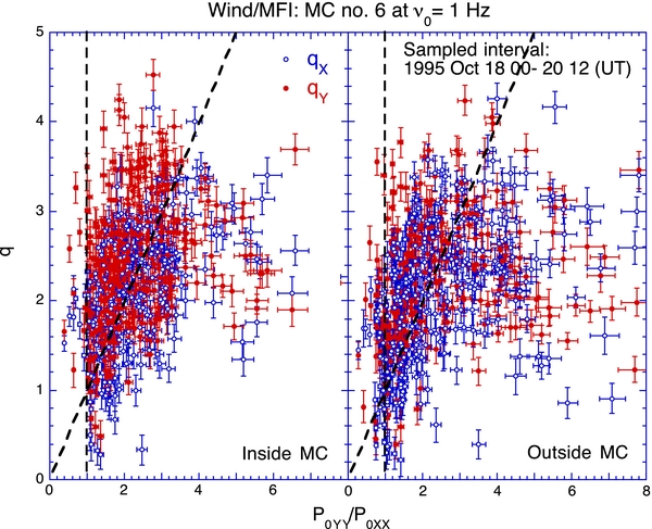
Figure 5. PSD spectral indices (q) are plotted vs. P0YY/P0XX inside (left panel) and outside (right panel) MC no. 6.
Download figure:
Standard image High-resolution imageLeamon et al. (1998a) noted that a flattening of Wind/MFI high frequency power spectra is evident at ν0 > 1 Hz and is more evident in intervals with a lower power level and a higher Nyquist frequency. We (Tan et al. 2011) also noted that, in the dissipation range, the deviation of the log(P) versus log(ν0) plot from the linearity is associated with the noise level of observations, which becomes more significant when the amplitude of PSDs is smaller. Since in the top panel of Figure 3, P0XX is often less than P0YY, the background effect on qX should be more serious than on qY. We hence assume q = qY in further analysis.
By assuming q = qY, inside the MC, we found that the fraction of observed ∼six minute subintervals, which satisfy Equation (10) and provide a calculable r value, is εr ∼ 61%. In the fourth panel of Figure 3, we compare P0YY/P0XX with qY. It can be seen that between two adjacent observed points with a time separation of ∼6 minutes, the P0YY/P0XX value could jump from ∼qY to ∼1 or verse versa, causing the amplitude fluctuation of r between ∼0 and ∼1 according to Equation (9).
Finally, we show the time profiles of θBV (the red line for all sampled subintervals) and r (blue lines for the subintervals where r is calculable) in the bottom panel of Figure 3. In view of its large amplitude fluctuation, we plot r by using a light blue thick line. In addition, we plot the weighted average trend of r by using a dark blue line. It can be seen that large amplitude fluctuations in r are superimposed on the top of an overall trend of r. The overall trend of r is consistent with that of θBV, indicating that the variation is mainly due to the effect of magnetic field orientation.
2.3.4. Comparison of Slab Fractions in Three MC Events
Plots similar to Figure 3 have been completed for the MC events no. 32 and no. 81 as shown in Figures 6 and 7, respectively. The common features of Figures 3, 6, and 7 can be summarized as follows.
- 1.In the three MC events examined, we often observe qY > qX > qZ.
- 2.HigherP⊥/P|| = (P0XX + p0YY)/P0ZZ and lower plasma β values are the common feature of MCs (Zank & Matthaeus 1992). However, inside MCs, theP⊥/P|| value in the dissipation range is less than that in the inertial range (Leamon et al. 1998b), indicating the decreased importance of transverse fluctuations and relative increase of compressive component in the dissipation range.
- 3.In the three MC events examined, the overall trend of r is consistent with that of θBV. However, because of large amplitude fluctuations in r, a smaller θBV value may link to a larger r value, although a larger θBV value often corresponds to a larger r value.
- 4.In the outer region of MCs, the r value is often larger than that in the MC center because a larger θBV value usually appeared in the outer region, given that the rotation of MC magnetic field is from the most southward to the most northward (or verse versa), in general. However, the mean value of r in the MC center never reaches zero as claimed by Leamon et al. (1998b).
- 5.Inside MCs, the fraction εr of observed ∼six minute subintervals, in which r is calculable, is (58 ± 3)% among the three MC events listed in Table 1.

Figure 6. Same as Figure 3 but for MC no. 32.
Download figure:
Standard image High-resolution image
Figure 7. Same as Figure 3 but for MC no. 81.
Download figure:
Standard image High-resolution imageOur observations described above could be helpful in understanding the characteristics of solar wind turbulences, in general. Further statistical study on magnetic fluctuations inside MCs is necessary. However, it is beyond the scope of this work, whose main task is to explore the relation between the observed L0eIII value of solar non-relativistic electron events and the turbulence geometry.
3. DISCUSSION
3.1. Dependence of Calculated Slab Fractions on the Width of Sampled Subintervals
Matthaeus et al. (1986) examined the effect of width Δt of sampled subintervals on the ensemble average. Contrary to an intuitive conjecture that increasing the width of sampled subintervals could improve statistics, Matthaeus et al. (1986) pointed out that wider samples might behave more unlike the ensemble average. This is because the behavior of an ensemble is consistent with the notion of stationarity about a local, well-defined mean magnetic field direction, while the systematic variations in field directions would violate such stationarity. However, since the width of subintervals (15 hr–16 days) analyzed by Matthaeus et al. (1986) is much wider than that examined by us, their conclusion cannot be directly applied to our analysis.
We hence carry out an observational examination of magnetic turbulence parameters deduced at different Δt values in order to find a proper Δt0 value in the frequency range of ν0 = 0.67–1.5 Hz. From the bottom panel of Figure 3, it can be seen that large amplitude fluctuations in r (the light blue line) are superimposed on top of an overall trend of r (the dark blue line). The overall trend of r can be calculated by using a locally weighted least-squared error method (Chambers et al. 1983) from the r values deduced at different N (Δt) values of each subinterval. As a result, at different N (Δt) values, the weighted average value rN(i) given at the reference point i (i = 1, n) can be estimated through interpolation. In order to compare rN(i) values at different N, the time separation of reference points is set at 6.28 minutes.
Because of the role played by both P0YY/P0XX and qY in the calculation of r (Equations (8) and (9)), for MC no. 6, we plot time profiles of weighted averaged P0YY/P0XX, qy, and r in Figure 8, starting from Δt > Δtm. It can be seen that rN(i) values given at N = 2048 (211, Δt = 3.14 minutes, the light green line), N = 4096 (212, Δt = 6.28 minutes, the red line), and N = 8192 (213, Δt = 12.6 minutes, the orange line) are consistent with one another, indicating that the deduced r values are stable between N = 211 and 213. We hence assume that the real r value is close to r0(i) = (r2048(i) + r4096(i) + r8192(i))/3 (i = 1, n). Consequently, the rms error σrN between rN estimated at N (Δt) and r0 is
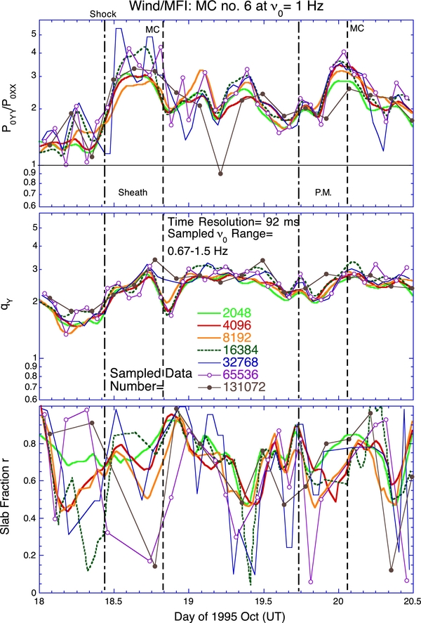
Figure 8. For MC no. 6, the time profiles of weighted averages of P0YY/P0XX (top panel), qY (middle panel), and r (bottom panel) deduced at ν0 = 1 Hz are shown for different sampled data numbers per subinterval.
Download figure:
Standard image High-resolution imageA similar examination on P0YY/P0XX, qy, and r is also carried out for the MCs no. 32 and 81. We then plot the deduced σrN values versus Δt (N) in Figure 9, which shows that the variation of σrN versus Δt is similar among the three MC events examined. In particular, a minimum of σrN ∼ 0.05 can be seen at N = 4096 (i.e., Δt0 = 6.28 minutes, which should be a proper choice of sampled subinterval width in our further analysis). Also, significant enhancement of σrN is seen when N > 16384 (214, Δt > 25 minutes).

Figure 9. The rms error, σrN, between the observed and expected weighted averaged values of r as given at ν0 = 1 Hz is plotted vs. the width Δt (i.e., the data number N per subinterval) of sampled subintervals. The correlation scale, Lc, deduced by Matthaeus et al. (2005) using ACE–Wind data with a time resolution of 1 minute, is reduced to the correlation time Tc (dashed line) by assuming the solar wind speed is 450 km s−1.
Download figure:
Standard image High-resolution imageMatthaeus et al (2005) examined the spatial correlation of solar wind turbulence by using two-point measurement from ACE–Wind data with a time resolution of one minute, which is just the time resolution Δtm of the mean magnetic field data used by us. Over a contiguous 24 hr period, they deduced a correlation scale Lc ∼ 0.0079 AU, which corresponds to the correlation time Tc ∼ 44 minutes, taking into account the mean solar wind speed being ∼450 km s−1 in the three MC events examined. The Tc value thus deduced is denoted in Figure 9 by the dashed line, across which σrN shows an increase of ∼4 times compared with that at Δt0, indicating that the mean magnetic field direction is no longer correlated when the time separation is grater than Tc. Therefore, excessive sampling as noted by Matthaeus et al (1986) should also appear in the frequency range examined in this work.
3.2. Comparison of Our Observations with Previous Works
To our knowledge, there have been very few reports on the turbulence geometry in MCs. Beside two case studies given by Leamon et al. (1998b) and Smith et al. (1999), there is a statistical study on an MC subset consisting of 393 sampling intervals from 28 MCs given by Hamilton et al. (2008).
Leamon et al. (1998b) examined the 1997 January 10–11 MC no. 12, which occurred when the Wind/MFI data have a higher sampling rate (τ0 = 46 ms). Leamon et al. (1998b) showed the time profile of the P⊥/P|| ratio, which is reproduced in the top panel of Figure 10, in the inertial range, where the ratio increased from 3.4 ± 0.5 before the sheath to 62 ± 9 inside the MC. However, they did not give the ratio in the dissipation range because of the noise level in the P0ZZ component. For the same MC event, the P⊥/P|| ratio deduced by us in the dissipation range is shown in the second panel of Figure 10, where we also show the real width Δt of each sampled subinterval. As explained in Section 2.3.3.1, most intervals have Δt0 = 6.28 minutes. The interval with Δt > Δt0 is due to data missing in the Wind/MFI archive. Comparing the second panel with the top panel, we note that the time variation tendency of the P⊥/P|| ratio in both the inertial and dissipation ranges is very similar. However, the ratio only increases from 2.3 ± 0.8 before the sheath to 4.8 ± 3.0 inside the MC, indicating a faster dissipation of transverse power occurring in the dissipation range (Leamon et al. 1998b).

Figure 10. For MC no. 12, the time profiles of the transverse to parallel power ratio (P⊥/P|| = (P0XX + P0YY)/P0ZZ) given by Leamon et al. (1998b) in the inertial range (top panel), the ratio given by us in the dissipation range as well as the real width Δt of sampled subinterval (second panel), and the slab fraction r and θBV given by us in the dissipation range. The top panel is reproduced from Leamon et al. (1998b) with the division of regions given by the original authors. In addition, for MC no. 34, the time profiles of the P⊥/P|| ratio given by Smith et al. (1999) in the inertial (oval) and dissipation (rectangle) ranges (fourth panel), the ratio given by us in the dissipation range as well as Δt (fifth panel), and r and θBV given by us in the dissipation range (bottom panel). The fourth panel is reproduced from Smith et al. (1999) with the data points in the dissipation range connected by us, using straight lines for clarity.
Download figure:
Standard image High-resolution imageAlso, in the dissipation range, Leamon et al. (1998b) found r =  and r =
  before and inside the MC, respectively. Their deduced r value shows a tendency to be close to 1 or 0. In contrast, for the same MC event in the dissipation range, our deduced r and θBV values are shown in the third panel of Figure 10, where r = 0.45 ± 0.35 and r = 0.66 ± 0.26 before and inside the MC, respectively. Therefore, further study is necessary in order to clarify if excessive sampling could cause the divergence.
The other MC case is the 1998 June 24–25 MC no. 34 examined by Smith et al. (1999). The time profiles of P⊥/P|| ratios shown by Smith et al. (1999) in both the inertial and dissipation ranges are reproduced in the fourth panel of Figure 10, where we connected the data points in the dissipation range by using straight lines for clarity. It appears that the P⊥/P|| ratios of Smith et al. (1999) in both the inertial and dissipation ranges are close to each other, which is inconsistent with the difference of the ratio in MC no. 12 (see the top and second panels in Figure 10). Also, the statistical study on the MC subset in Hamilton et al. (2008) shows contradictory results on the r estimation in the dissipation range. When the input parameters of Equation (9) are taken from individual observation points, they obtained r = 0.83 ± 0.01 and r = 1.0000 ± 0.0002 in the open field line and MC cases, respectively. On the contrary, when the input parameters are taken from the ensemble average over a given θBV interval, they obtained r =  and r =
  in the open field line and MC cases, respectively. In contrast, for all five MC events analyzed in this work, we obtain the mean r = 0.61 ± 0.12 inside MCs, which is consistent with the ensemble averaged value found by Hamilton et al. (2008). Since Smith et al. (1999) and Hamilton et al. (2008) also used Δt ⩾ 1 hr of sampled subintervals in their works, further study is also necessary in order to clarify the divergence of r calculation in the dissipation range.
3.3. What Causes the Failure of Slab Fraction Calculations?
In the existing composite slab/2D model (Bieber et al. 1996), Equation (10) must be satisfied in order to calculate the slab fraction r. However, ∼42% of the observed subintervals, which are evenly distributed along the time axis, do not satisfy Equation (10) and provide a calculable r value. What causes the failure of the r calculation? Is the nature of turbulence in the interval where r is calculable the same as that in the interval where r is indeterminate? Would the r-missing interval affect the estimation of time variation of r?
While r may not be calculated within a time subinterval, the P⊥/P|| = (P0XX + P0YY)/P0ZZ ratio is always calculable. Therefore, we examine the characteristics of the P⊥/P|| ratio in order to identify the nature of turbulence. In the inertial range, Smith et al. (2006) analyzed the variation of the P⊥/P|| ratio with the plasma β. They found that the variation is most likely due to the turbulent cascade of noncompressive fluctuations that drives a degree of compressive fluctuations within the turbulence. Hamilton et al. (2008) extended the analysis to include the dissipation range. They noted a weaker dependence of the P⊥/P|| ratio with the plasma β in the dissipation range. It has been unclear whether the weaker correlation is just a remnant from the inertial range cascade combining with the onset of dissipation or if it is reflective of true dissipation range dynamics.
Regardless of the dynamics that causes the correlation, the variation of the P⊥/P|| ratio with the plasma β could be used to identify the nature of turbulences among different subintervals. For the three MC events listed in Table 1, we plot theirP⊥/P|| ratio versus the plasma β in Figure 11, where the red solid dots and blue open circles denote all data and the data whose r is calculable (note that the blue circle would mask the red dot), respectively. Each event has a 2.5 day examining period in which we did not differentiate between inside and outside MCs in order to increase statistics. From the figure, it can be seen that turbulence in all subintervals, regardless of r being calculable or indeterminate, satisfies the same relation between theP⊥/P|| ratio versus the plasma β, implying a common nature. Also, for the three MC events examined, we find the averaged value of the slope for the log(P⊥/P||) versus log(β) plot is −0.27 ± 0.10, which is close to the result (–0.17 ± 0.02) of Hamilton et al. (2008) for the MC subset in the dissipation range. Since the observed turbulence has a common nature, we would expect that the presence of r-missing intervals does not affect the estimation of the time variation of r.
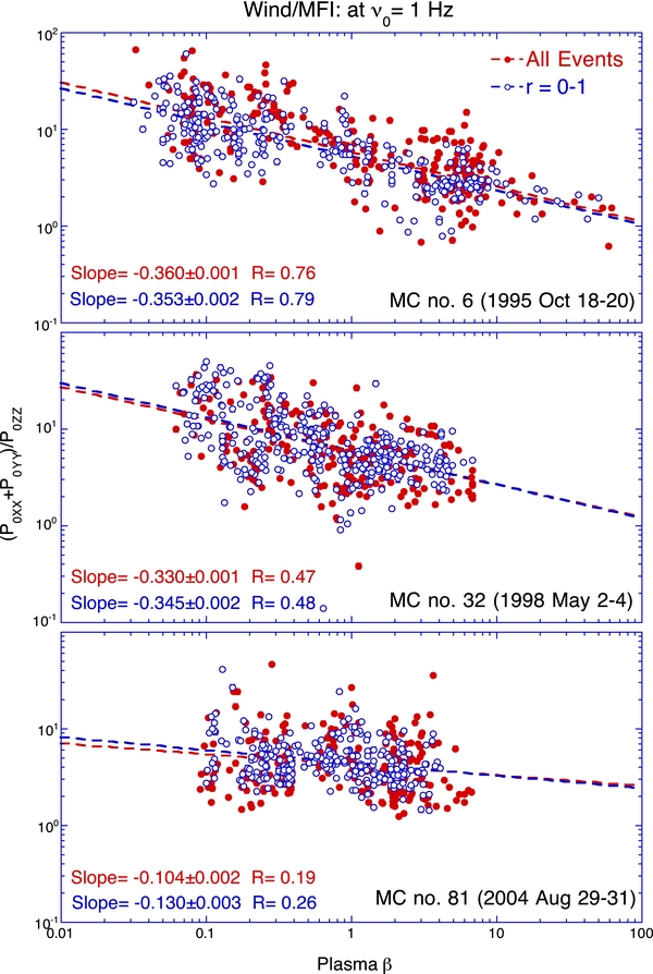
Figure 11. Ratio of transverse to parallel power (P⊥/P|| = (P0XX + P0YY)/P0ZZ) given at ν0 = 1 Hz is plotted vs. the plasma β for the three MC events listed in Table 1. The slope is the least-squares fitting result between log((P0XX + P0YY)/P0ZZ) and log(β).
Download figure:
Standard image High-resolution imageWe then check what causes the failure of the r calculation, which exhibits as P0YY/P0XX > qY in Figure 3. We plot log((P0YY/P0XX)/qY) versus the logarithmic value of various plasma parameters to check any possible correlation between them. No significant correlation of (P0YY/P0XX)/qY with the main plasma parameters (e.g., the solar wind speed (Vsw), proton temperature (Tp), plasma β, etc.) has been found. However, there are correlations of (P0YY/P0XX)/qY with the transverse power (P⊥ = P0XX + P0YY) and the proton number density (Np) as shown in the left and right panels of Figure 12, respectively, where observed points located above the dashed horizontal line indicate the failure of r calculation. It can be seen that the increased portion of r failure is correlated with the increase of P⊥ or Np. Because the total number of observation points is 555, the correlation coefficient R = 0.31 and 0.22 in the left and right panels of Figure 12 correspond to the probabilities, P, at which no correlation exists, being 4.4 × 10⁻⁸ and 2.1 × 10⁻⁷, respectively.

Figure 12. Plots of log((P0YY/P0XX)/qY) as given at ν0 = 1 Hz vs. log(P0XX + P0YY) (left panel) and log(Np) (right panel), where Np is the proton number density, are shown for MC no. 6 with the dashed red line being the least-squares fitting result.
Download figure:
Standard image High-resolution imageSince IMF turbulence is well correlated with the solar wind density fluctuation and the solar wind density itself is a reasonable proxy of its fluctuation (Richardson et al. 1998; Richardson & Paularena 2001), the correlation of (P0YY/P0XX)/qY with Np is equivalent to the correlation of (P0YY/P0XX)/qY withP⊥. Therefore, Figure 12 indicates that the failure of the r calculation could be due to the increased magnitude of transverse turbulence that violates the simplified assumption in the existing model (Equation (9)), including the symmetry between the x and y axes. Further development of theoretical models, which is beyond the scope of this work, could include more observed subintervals into the calculation of r.
3.4. Comparison of the Slab Fraction with L0eIII
Having deduced the r value, we plot the time profiles of r and r(P0XX + P0YY), the effective power in scattering electrons, for the three MC events listed in Table 1, in Figure 13, where an expanded time scale only covering a 10 hr interval around the occurrence of impulsive electron events is shown. In the top two panels of Figure 13, we show MC no. 6, where r(P0XX + P0YY) ∼ P0XX + P0YY because of r ∼ 1. The error bar of r is estimated by using the bootstrap method (Efron & Tibshirani 1991) in which all input parameters (q, P0XX, P0YY, and θBV) in Equation (9) are assumed to be random numbers satisfying the Gauss statistics, and the mean and standard deviation of r are deduced after 1000 computations.
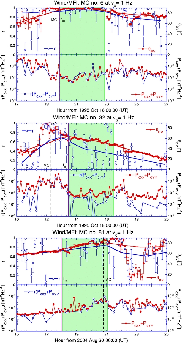
Figure 13. Details of time profiles of r and θBV, as well as of r(P0XX + P0YY) and P0XX + P0YY given at ν0 = 1 Hz, are shown for the three MC events listed in Table 1. The dashed line and light green band are the location of MC boundary and the time interval of impulsive electron events, respectively.
Download figure:
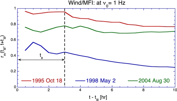
Standard image High-resolution imageWe then estimate the mean r value experienced by non-relativistic electrons. In an impulsive electron event, higher energy electrons (Ee ∼ 100 keV) could reach the observer in 1 AU soon after tIII, while lower energy electrons (Ee ∼ 10 keV) should reach 1 AU after a delay, t. The interval-averaged rm(tIII, t + tIII),

gives the mean r value experienced by all electrons. As shown in Figure 14, for the three MC events listed in Table 1, a more or less constant rm(tIII, t + tIII) value shows in the interval of te = t − tIII = 3 hr, which is denoted by the dashed line. We will estimate the mean r value over this interval, which is also denoted in Figure 13 by the light green band, because lower energy (Ee ∼ 10 keV) electrons could travel scatter-free a distance of ∼4 AU within such a time interval.
Figure 14. Average rm(tIII, t + tIII) value of the slab fraction estimated between tIII and t + tIII is plotted vs. t − tIII for the three impulsive electron events listed in Table 1. The interval width of the occurrence of impulsive electron events is assumed to be te.
Download figure:
Standard image High-resolution image
Therefore, from the assumed sampled interval width te, we deduced the mean r and r(P0XX + P0YY) values as listed in Table 1. It can be seen that the r(P0XX + P0YY) value is comparable among the three MC events examined. Actually, the upper limit of r(P0XX + P0YY) in MC no. 6 is slightly higher than that in the other two events, although the L0eIII value in MC no. 6 is the largest. It is evident from Table 1 and Figure 13 that, in order to observe L0eIII > 3.2 AU, we should have the slab fraction r in the dissipation range being close to 100%.
3.5. Implication of Our Observation
First, we need to point out that in Section 2.3.3.2, the observed large amplitude fluctuation in the slab fraction r is superimposed on top of an overall trend of r. However, in Section 3.4, we only examine the overall trend of r by averaging r over the occurring interval of impulsive electron events. This is because the onset time of solar impulsive electron events is dispersive relative to electron energies, as the transport time of electrons from their release site near the Sun to the observer depends on the velocity of electrons. Nevertheless, it should be emphasized that large amplitude fluctuations in r are also a physical reality as explained in Section 2.3.3.2. The drastic change of r between two adjacent observed points with a time separation of ∼6 minutes may provide a physical basis to explain the "dropout" observation of energetic ions (Mazur et al. 2000; Chollet & Giacalone 2008) and low-energy electron bursts as well as electron strahls (Gosling et al. 2004), where dispersionless modulation in particle intensities is found over various energy ranges of particles.
The difference between the slab and 2D turbulence components in the solar wind could be used to explain the dropout observation. According to Ruffolo et al. (2003), as the solar wind expands, magnetic flux tubes that remain trapped within regions dominated by the 2D turbulence could form small-scale filamentary structures, whereas flux tubes dominated by the slab turbulence should be diffused. In contrast, Zimbardo et al. (2004) and Pommois et al. (2005) suggested that the dominance of the slab turbulence would cause SEP concentration, leading to the observed dropout of low-energy ions. Recent works by Trenchi et al. (2013a, 2013b) identified magnetic field topologies that might be associated with the borders of dropout events and the maxima of SEP intensities.
Here, we analyze whether our observation could be explained based on the property of solar wind turbulence. Although our observation is motivated by Smith et al. (1999), the conclusion deduced from it is opposite to their claim that in MCs the L0eIII value should increase with the increase of 2D turbulence fraction. In fact, their claim is based on the assumption (see Section 1.3) that only the slab component with its wave vector k∥Bm resonantly scatters charged particles, whereas the 2D component with its wave vector k⊥Bm does not scatter particles. However, before going to examine the transport of charged particles along the magnetic flux tube, we should first analyze how the spatial structure of magnetic flux tubes is formed. In particular, could the geometry of solar wind turbulence affect the structure?
According to Zimbardo et al. (2004), the spatial structure of magnetic flux tubes depends on the turbulence level δB/Bm, where δB is the field fluctuation, and the turbulence anisotropy that is characterized by the slab fraction r. In the solar wind, δB/Bm is of the order of 0.5–1.0. When the 2D component is dominant (r ∼ 0), the flux tube evolves very quickly, forming very fine, diffusive structures. On the contrary, when the slab component is dominant (r ∼ 1), the flux tube evolves slowly, executing large coherent transverse displacements.
Furthermore, charged particles behave largely as test particles streaming along the turbulent magnetic field, which plays the role of a guiding channel for energetic particles. Pommois et al. (2005) examined the spatial distribution of protons with 1–104 MeV energies. They found that at relatively low energies (1–10 MeV), the proton distribution closely follows the magnetic flux tube structure. However, at higher energies, the protons are less tied to the flux tube. This is because the effect, such as the grad-B drift, would increase with the increase of proton gyroradius. Therefore, the spatial distribution of protons should resemble the shape of magnetic flux tubes up to about 10 MeV.
While the existing turbulence analysis has concerned energetic ions in the inertial range of the PSD spectrum, our observation is related to non-relativistic electrons in the dissipation range. Nevertheless, the existing simulation could provide a qualitative understanding on the spatial structure of magnetic flux tubes involved in the transport of non-relativistic electrons, in view of large parameter ranges used in the simulation (see, e.g., Matthaeus et al. 2003; Zimbardo et al. 2004). In addition, because of very small gyroradius of non-relativistic electrons (for example, ∼27 keV electrons in an ∼5 nT magnetic field only have their gyroradius of ∼100 km), the spatial distribution of non-relativistic electrons should be closer to the spatial structure of magnetic flux tubes than low-energy ions. Consequently, it could be expected that when the slab component is dominant (r ∼ 1), the flux tubes should be closed and regular for very long transport distances of particles (Zimbardo et al. 2004).
Therefore, our observation is understandable by taking into account the characteristics of solar wind turbulence; especially when only the slab spectral component exists, magnetic flux tubes (magnetic surfaces) are closed and regular for very long distances along the transport route of particles (Matthaeus et al. 1995, 2003; Bieber et al. 1996; Zimbardo et al. 2004).
Finally, a question remains: in the case that the magnetic flux tube has collapsed at r ∼ 0, why do non-relativistic electrons still propagate along the Parker spiral line with L0eIII ∼ 1.2 AU, as seen in the MC event no. 32? It could be due to the fact that in the stable solar wind condition, the Parker spiral line should be the shortest path of particles from their injection site near the Sun to the observer at 1 AU. More observations and simulations are necessary in order to answer this question.
4. SUMMARY
Three MC events, in which impulsive solar electron events occurred in the highly wound outer region, are employed to investigate the difference of path lengths, L0eIII, traveled by non-relativistic electrons from their release site near the Sun to the observer at 1 AU. Our main findings are as follows.
- 1.Assuming that electron injection occurs at the onset time of type III RBs, from the Wind/3DP/SST electron data, we have deduced the L0eIII value ranging from ∼1.3 to ∼3.3 AU.
- 2.By examining the correlation of L0eIII with the IP scattering condition, we find that a negligible IP scattering level can be seen in both L0eIII > 3 AU and ∼1.2 AU events, indicating that the difference of L0eIII could be linked to turbulence geometry (slab or two-dimensional) in the solar wind.
- 3.By using the high time resolution Wind/MFI magnetic field data, we examine the PSDs of magnetic fluctuations in the mean magnetic field coordinate system. In our examination, we take ∼six minutes of IMF sampled subintervals in order to improve the time resolution of the magnetic turbulence analysis in the dissipation range.
- 4.We have found that large amplitude fluctuations in the slab fraction r are superimposed on the top of an overall trend of r. The variation in the overall trend of r is consistent with that of θBV, which is the angle between the mean magnetic field and the solar wind velocity, indicating that the variation is mainly due to the effect of magnetic field orientation.
- 5.For the three MC events examined, we observe an increase of the slab fraction r in the transverse turbulence with increasing L0eIII value, reaching ∼100% in the L0eIII > 3 AU event.
- 6.Our observation implies that when only the slab spectral component exists, magnetic flux tubes (magnetic surfaces) are closed and regular for very long distances along the transport route of particles.
We gratefully acknowledge data provided by the NASA/Space Physics Data Facility (SPDF)/CDAWeb and Wind/3DP Data Center. Also, we thank K. Ogilvie, R. Lin, and A. Szabo for their support of this work, and the anonymous reviewer for valuable comments.