


ABSTRACT
We have investigated a supra-arcade structure associated with an M1.6 flare, which occurred on the south-east limb on 2010 November 4. It is observed in EUV with the Atmospheric Imaging Assembly (AIA) on board the Solar Dynamics Observatory, microwaves at 17 and 34 GHz with the Nobeyama Radioheliograph (NoRH), and soft X-rays of 8–20 keV with RHESSI. Interestingly, we found exceptional properties of the supra-arcade thermal plasma from the AIA 131 Å and the NoRH: (1) plasma upflows along large coronal loops and (2) enhancing microwave emission. RHESSI detected two soft X-ray sources, a broad one in the middle of the supra-arcade structure and a bright one just above the flare-arcade. We estimated the number density and thermal energy for these two source regions during the decay phase of the flare. In the supra-arcade source, we found that there were increases of the thermal energy and the density at the early and last stages, respectively. On the contrary, the density and thermal energy of the source on the top of the flare-arcade decreases throughout. The observed upflows imply that there is continuous energy supply into the supra-arcade structure from below during the decay phase of the flare. It is hard to explain by the standard flare model in which the energy release site is located high in the corona. Thus, we suggest that a potential candidate of the energy source for the hot supra-arcade structure is the flare-arcade, which has exhibited a predominant emission throughout.
Export citation and abstract BibTeX RIS
1. INTRODUCTION
The explosive energy release during solar flares results in heating of the surrounding plasma. This hot plasma contains crucial information that can be used to understand the physical processes occurring in flares. Supra-arcade (SA) structures, which appear above the flare loops, are intimately associated with the energy release process during the flare. These structures consist of hot plasma with a temperature of around 10 MK and have been observed in X-rays (Švestka et al. 1998; McKenzie & Hudson 1999; McKenzie & Savage 2000; Gallagher et al. 2002; McKenzie & Savage 2009; McKenzie 2013) and the EUV (Innes et al. 2003a, 2003b; Asai et al. 2004; Reeves & Golub 2011; Savage et al. 2012; McKenzie 2013). The SA structures generally appear as an extended diffuse structure, best viewed over the limb of the sun, and often accompany a coronal mass ejection. A fan arcade structure in X-rays is one representation of an SA structure that appears in long duration events. Švestka et al. (1998) found a fan structure of coronal rays above post-flare loops revealed by Yohkoh SXT. They suggested that the fan structure represents mass flows through open fields rooted in the associated active region, flowing out into the interplanetary space as a form of the solar wind. Alternatively, McKenzie & Hudson (1999) suggested that the fan structure might involve a current sheet involving a magnetic reconnection process inside of it. They found that violent lateral motions within the fan structure occurred as a response to downflows of dark X-ray voids, which are called SA downflows (SADs). With regard to the SADs, they inferred that it is evidence of outflows caused by a magnetic reconnection process from a high altitude of the corona (See Forbes & Acton 1996).
In X-rays, Gallagher et al. (2002) reported observations of a SA structure from RHESSI (Lin et al. 2002). RHESSI images revealed an extended X-ray source that slowly moved to greater heights in the corona over several hours. Since in the standard flare model (Forbes & Acton 1996), magnetic reconnection takes place at x-point within a current sheet in the corona, the observed motion of the SA source is attributed to a moving energy release to higher altitudes. They considered that the x-ray source of SA structure, during the decay phase of the flare, is a hot thermal source filling hot loops based on the standard flare scenario explained above.
Recently, the hot plasma in the corona has been monitored by six EUV channels of Atmospheric Imaging Assembly (AIA; Lemen et al. 2012) on board the Solar Dynamics Observatory (SDO). Because of the narrowband response, high sensitivity, and high-spatial resolution of AIA, the diffuse and nebulous SAs were visible in exquisite detail, particularly in the 131 Å passband, which has a peak temperature response at 11 MK. Using AIA observation, Reeves & Golub (2011) reported three events representing hot SA structure and proposed that the hot plasma is in a region of weak magnetic field surrounding the current sheet, allowing the morphology to be more diffuse than the post-flare loops (see Yokoyama & Shibata 1997; Reeves et al. 2010). Savage et al. (2012) analyzed one of their events in detail using AIA imaging data. In their results, they found inflows and outflows in and near the SA and suggested them to be evidence of the magnetic reconnection in the current sheet. McKenzie (2013) confirmed the existence of turbulent flows involving vortical-like flow within the hot SA structure. There have been many valuable investigations of SA structures from a morphological and dynamical point of view based on EUV and X-ray observations. Nevertheless, the identification and generation mechanism of SAs are unknown.
In this paper, we present an investigation of a thermal SA structure and a flare-arcade (FA) associated with a limb flare which occurred on 2010 November 4. This is one of the events reported by Reeves & Golub (2011). This event is unique because it is the only one of its type for which high-resolution EUV images obtained by AIA, 17 GHz microwave images by Nobeyama Radioheliograph (NoRH; Nakajima et al. 1994), and X-ray observations from RHESSI are simultaneously available. Furthermore, we found unusual properties, such as successive plasma upflows and an increase of microwave emission, which have not yet been reported. Data processing and analysis for this investigation were performed using SolarSoft software (Freeland & Handy 1998). In Section 2, we describe the multi-wavelength observations and the morphological evolution of the event. In Section 3, we present our analysis and results for the physical parameters related to the SA structure and the FA. Lastly, in Section 4, we discuss where and how the hot plasma was generated and injected into the SA structure.
2. OBSERVATIONS
We have examined an M1.6 flare that occurred near the southeast limb on 2010 November 4, in active region NOAA11121. In the top panel of Figure 1, a time profile of the GOES soft X-ray flux shows that the flare started at 23:52, peaked at 23:57, and gradually decreased until another flare began at 00:50 on the fifth. The middle and bottom panels of Figure 1 show light curves from NoRH (Nakajima et al. 1994; Takano et al. 1997) and RHESSI (Lin et al. 2002), respectively. The detailed observations for the FA and SA structure are given according to wavelengths.
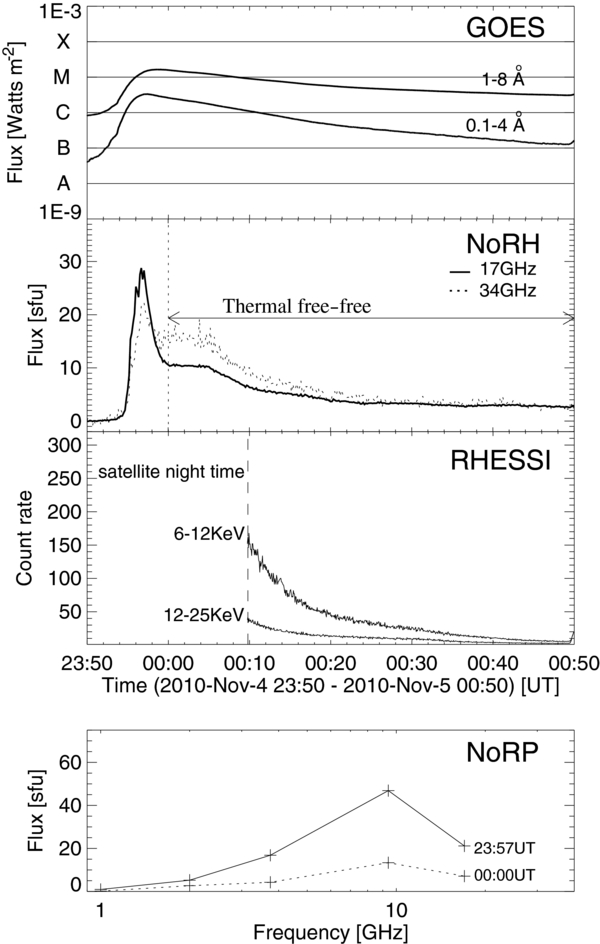
Figure 1. From the top, GOES X-ray flux curves of M1.6 limb flare in low energy band 1–8 Å and high energy band 0.5–4 Å, the time profile of microwave flux of NoRH 17 (solid line) and 34 GHz (dotted line) integrated for the field of view of Figure 4, RHESSI X-ray counts rate for 6–12 keV (upper line) and 12–25 keV (lower line), and microwave spectrums observed by NoRP multi-channels 1, 2, 3.75, 9.4, and 17 GHz at the flare peak time of 23:58 UT November 4 (solid line) and 00:00 UT November 5 (dashed line).
Download figure:
Standard image High-resolution image2.1. EUV Observations
The AIA instrument on board SDO has six narrowband EUV channels that are sensitive to different ionization states of iron (Boerner et al. 2012). The AIA produces high spatial resolution images (1 2) every 12 s. Figure 2 shows multi-thermal structures observed by the AIA at ∼00:20, during the decay phase of the flare. In two of the channels, 131 Å and 94 Å, the images clearly reveal a SA structure situated above the FA and extending to the high corona. For a flare, the AIA 131 Å channel contains a contribution from Fe xxi, formed at 11 MK, while the 94 Å channel contains lines from Fe xviii, formed at 7 MK (Lemen et al. 2012). At the same time, these channels also contain a significant response to cooler plasma temperatures of ∼1 MK. Therefore, one should be careful when estimating, even roughly, the temperature of the plasma using these two filters. Luckily, the AIA 171 Å and 193 Å bandpasses have temperature response curves which peak around the temperature range close to the lower temperature components of the 131 Å and 94 Å channels (see Figure 11). Since there is no emission consistent with the SA structure in these two channels (Figure 2), only the very hot plasma, over at least 7 MK, fills the SA structure. On the other hand, the FA are observed at all wavelengths, where they appear at growing heights as time progresses. The evolution of the flare in all AIA wavelengths is available as a mpeg movie in the electronic edition of the journal. In the movie, the AIA 131 Å and 94 Å channels show that the hot plasma extended toward the high corona. In the case of the 335 Å channel, the region of hot plasma appears dark due to an absence of 2.5 MK plasma, which is the peak temperature response of this channel. In the other three wavelengths, coronal loops around the flare expanded rapidly and swayed.
Figure 2. Observations of six EUV channels of the AIA taken around the middle of the decay phase.
An animation of this figure is available.
Download figure:
Video Standard image High-resolution imageFigure 3 shows a sequence of snapshots taken by the AIA 131 Å channel. At the flare onset (Figure 3(b)), small-scale flare loops brighten, and the hot plasma above the flare loops stretches out toward the high corona. After the flare peak, the FA comes into view with rising motion, and the SA structure stops expanding and brightens gradually, with flows observed along two slits denoted by Flow A and Flow B in Figure 3(d). Figure 4 shows the position versus time stackplots, which we constructed by extracting ten-pixel wide slits of Flows A and B. These stackplots demonstrate that the flows of the hot plasma are upward and continuous at the particular positions during the decay phase. Anti-sunward flows in the SA structure are contrary to sunward SADs from McKenzie & Hudson (1999) and Gallagher et al. (2002) in their directionality. Also, it seems clear that it differs from the turbulent flows confirmed by McKenzie (2013). However, the upflows and SADs might have an identical mechanism, such as the magnetic reconnection process which can produce bidirectional outflows. Estimated flow speeds gradually decreased from 380 km s−1 at 00:12 UT to 100 km s−1 at 00:34 UT for Flow A and from 630 km s−1 at 00:12 UT to 135 km s−1 at 00:31 UT for Flow B. In the late decay phase (Figure 3(f)), the emission from the FA steeply decreases, while the SA structure shows continuous emission from the hot plasma.
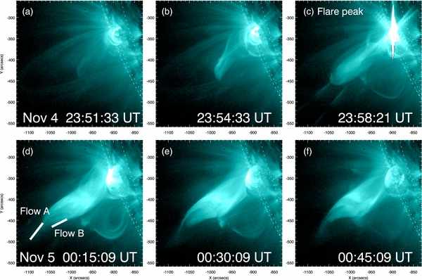
Figure 3. Time sequential images of AIA 131 Å taken (a) before onset, (b) at onset, (c) at the peak of the flare, and (d–f) during the decay phase. The regions of upflows are marked by two slits in (d) and stated by Flow A and Flow B, respectively.
Download figure:
Standard image High-resolution image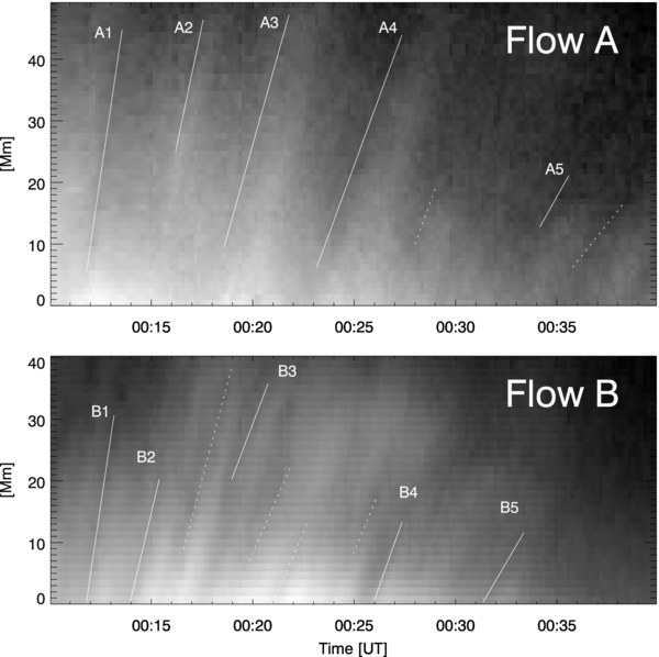
Figure 4. Time vs. space stackplots made by extracting two slits, Flow A (top) and Flow B (bottom) depicted in Figure 3(d). The y-axis is the space along the slit and toward the high corona. The front of propagating bright features is fitted by solid lines and represents successive upflows with decreasing speeds during the decay phase of the flare. Estimated speeds are as follows: Flow A, A1 = 375 km s−1, A2 = 180 km s−1, A3 = 200 km s−1, A4 = 150 km s−1, and A5 = 100 km s−1; and for Flow B, B1 = 630, B2 = 245 km s−1, B3 = 110 km s−1, B4 = 180 km s−1, and B5 = 135 km s−1.
Download figure:
Standard image High-resolution imageSome of this hot plasma may be expelled out from the sun to the interplanetary space in the form of upflows and/or may cool down and fall back to the surface. Before the flare start time, SOHO/LASCO observations from CDAW data center5 revealed sunward flows of dark voids at around 23:16 UT on November 4. We note that these flows could interact with the SA structure but there is no evidence of such flows in the AIA data during the flare. On the other hand, Figure 5 shows that the bundle of coronal loops (indicated by two white arrows) at 193 Å connected to Flow A at 131 Å. Also, Flow B showed curved streaming as if it follows an existing field line in the SA structure (see the mpeg movie of the electronic edition of journal). Thus, we suggest that the SA structure consists of a thick coronal loop confining the hot plasma at the loop apex and large-sized loops passing the hot plasma to the other site. This hot plasma might be supplied from the SA structure itself or the lower part of the SA structure, most likely from the FA, which is the only remarkable emission source below the SA structure.

Figure 5. AIA 193 Å image and AIA 131 Å contour (blue) taken at 00:45 UT. The Flow A slit is located on the large-sized coronal loops, which is denoted by white arrows, revealed in the AIA 193 Å image.
Download figure:
Standard image High-resolution image2.2. Microwave Observations
NoRH provides microwave imaging data at two frequencies, 17 and 34 GHz, with a spatial resolution of 10'' and 5'', respectively. We synthesized microwave images with a cadence of 10 s. To improve the signal-to-noise ratio of the 34 GHz images, 30 images are averaged over 5 minutes during the decay phase. The second panel of Figure 1 shows the spatially integrated flux at 17 and 34 GHz over the flare region exhibited in Figure 6. The impulsive phase of the flare shows a drastic increase and decrease in flux, which peaked at 23:57 UT. Then, a gradual decrease starts around 00:00 UT (vertical dashed line in the second panel of Figure 1).

Figure 6. Time sequential maps of brightness temperature (TB) of 17 GHz with TB contours of 34 GHz (blue) observed by Nobeyama Radioheliograph: (a) onset, (b) peak of the flare, and (c–f) during the decay phase. The contour levels are 10%, 50%, and 90% of the maximum TB at 34 GHz.
Download figure:
Standard image High-resolution imageFigure 6 shows sequential maps of brightness temperature (TB) at 17 GHz with 34 GHz TB contours over plotted. Figures 6(a) and (b) are taken at the onset and the peak of the flare, and Figures 6(c)–(f) are obtained during the decay phase. At the peak of the flare, the bright NoRH source corresponds to the flare loops seen by AIA, which is revealed as the FA during the decay phase, and the position of maximum brightness is coincident with the top of the flare loops. Simultaneously, a weak but clear blob-like structure appears at a greater height, above the bright loop-top source. During the decay phase, the blob-like structure stretches out and fills the region of the SA structure shown in the AIA 131 Å image. The TB of the SA structure increases, while the brightness of the flaring source decreases (Figures 6(c)–(f)). This can be seen more clearly in Figure 7, which shows the time profile of brightness temperature at 17 and 34 GHz for two regions, the top of the FA and the SA structure, which are denoted by white boxes in Figure 6(f). During the decay phase from 00:00 UT, TB in the FA exhibits a decreasing pattern, while TB in the SA clearly increases up to 1.9 × 10⁴ K at 17 GHz and 5 × 10³ K at 34 GHz. For the 34 GHz emission, the SA structure was seen just after the middle of the decay phase, ∼00:20 UT.

Figure 7. Time profile of the brightness temperature in the top of the flare-arcade (FA) and the supra-arcade (SA) structure obtained by NoRH 17 and 34 GHz. The SA in 34 GHz is seen in the middle of the decay phase.
Download figure:
Standard image High-resolution imageNoRH observations provide an opportunity to derive a spectral index, α (log [Flux34/Flux17]/log [34 GHz/17 GHz]), for spatially resolved regions. Gyrosynchrotron emission leads to α < 0 and thermal free–free emission leads to α ∼ 0 in the high-frequency regime (see Dulk 1985). Figure 8 shows time variation of index α derived from the SA and the FA. For the SA, the α index is valid only after 00:20 UT when the SA emission is observed at 34 GHz. The index α is around –1 at the flare peak time, while it goes to ∼0 during the decay phase. It is apparent that the radio emission comes from gyrosynchrotron during the impulsive phase, while it comes from thermal free–free and optically thin plasma during the decay phase. This is reconfirmed from microwave spectra in the bottom panel of Figure 1, which are taken by NoRP (Nakajima et al. 1985) multiple channels at 1, 2, 3.75, 9.4, and 17 GHz. At the flare peak time, the spectrum exhibits a turnover frequency between 9.4 and 17 GHz (solid line), and in the early decay phase, 00:00 UT, the spectrum becomes flat, e.g., α ∼ 0 (dashed line).

Figure 8. Time profile of the alpha index at the top of the flare-arcade (FA) and the supra-arcade (SA) structure.
Download figure:
Standard image High-resolution imageWith regards to the microwave emission of the SA structure, Nakajima & Yokoyama (2002) presented microwave observations of a collimated ejection which occurred above a flare loop and lasted for several minutes. The authors suggested it was caused by an injection of high-energy electrons, which may have been generated by the magnetic reconnection of a jet. This is the only example that clearly shows microwave emissions extended above the flare loops and off-limb of the sun similar to our event. However, our event shows an increase of microwave emissions over a long time (∼1 hr), while Nakajima & Yokoyama (2002) studied short lasting structure, and thus they differ in kind.
2.3. X-Ray Observations
RHESSI observes X-ray and γ-ray photons in the energy range 3 keV to 17 MeV. The instrument is capable of both (separate and combined) imaging and spectroscopy with a spatial resolution of 23 and an energy-dependent spectral resolution of ∼1–10 keV. Unfortunately, there is no data available during the impulsive phase of the flare due to satellite night. During the decay phase, low-energy photons were observed in the 6–20 keV energy range (third panel of Figure 1), while there is no counts above background at energies greater than 20 keV.
RHESSI X-ray images reveal two coronal soft X-ray sources in the 8–20 keV energy range: a compact source near the limb (FA), located at the top of the flare loops; and a faint extended source high in the corona (SA), which is cospatial with the hot SA structure (Figures 9 and 10). The extended SA structure, however, is significantly weaker than the compact source. Due to the limitation of RHESSI's dynamic range, it is difficult to image the SA source in the presence of the bright compact source using the traditional CLEAN algorithm (Hurford et al. 2002). However, using the two-step CLEAN method described in Krucker et al. (2011), we are able to recover the SA source. Applying this method, the resulting compact and SA sources are reconstructed with spatial resolutions of ∼12'' and ∼35'' respectively. The Figure 9 shows both sources for two time intervals, 00:14:08–00:18:40 UT (red contours) and 00:41:30–00:44:30 UT (blue contours). The compact source contour values are 70%, 80%, and 90% of the compact source maximum intensity, while the extended source contours are 3.3%, 3.5%, and 3.7% and 27%, 28%, 29% of the compact source maximum intensity for two time intervals, respectively.
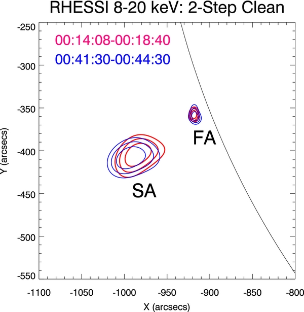
Figure 9. RHESSI X-ray imaging integrated by an energy range of 8–20 keV for 00:14:08–00:18:40 UT (red contour) and 00:41:30–00:44:30 UT (blue contour). X-ray images are constructed by the two-step CLEAN method. Bright source FA is constructed by fine grids, and faint and broad source SA is constructed by coarse grids.
Download figure:
Standard image High-resolution image
Figure 10. Combined image with AIA 131 Å image, TB contour of NoRH 17 GHz (blue), and RHESSI 8–20 keV (red) taken during the early decay phase.
Download figure:
Standard image High-resolution imageGallagher et al. (2002) has shown a similar examination of a SA structure using RHESSI data. During the decay phase of their event, a thermal source appeared high in the corona at an energy range of 6–25 keV, and the altitude of the source centroid moved to greater heights with a velocity of 9.9 km s−1. In our case, detailed imaging spectroscopy to recover the temperature and emission measure of the SA source is not possible, due to the low counting statistics, but RHESSI spectroscopy indicates that X-ray emission of the flare, which contains both the SA and FA source, is certainly thermal. The centroid of the SA source shifts around 10'' during the decay phase with a speed of around 38 km s−1 (Figure 9) but, unfortunately, the nature of the two-step CLEAN does not allow us to determine if this motion is real. Indeed, Gallagher et al. (2002) found hot thermal structure high in the corona and FA below it in EUV observation. However, during the decay phase, one X-ray source appeared just as high in corona. Thus, we presume that, in our event, the FA which has a predominant X-ray source might play a certain role for the formation of the SA as an energy source.
3. PHYSICAL PARAMETERS
Figure 10 shows a combination of multi-wavelength observations with an AIA 131 Å image, contours of NoRH 17 GHz (blue) at around 00:30 UT, and RHESSI soft X-ray contours from 8–20 keV integrated from 00:32–00:34 UT (red). The figure clearly shows that the RHESSI SA source is cospatial with the SA structure seen in EUV and microwaves, and the RHESSI FA source is located at the top of the FA. We have analyzed the physical parameters of the FA and SA based on observational results.
3.1. Temperature
To derive a plasma temperature, we used the two GOES X-ray channels (1–8 Å and 0.5–4 Å) for the FA source and AIA 131 Å and 94 Å images for the SA source (see Section 2.1). We have used observations from different instruments for each source due to the saturation effects on the FA region in AIA 131 Å images. However, since the FA region includes the flare loops, which are the main source of soft X-ray, it is reasonable to determine T of the FA using the ratio of the two GOES X-ray channels even though they are full-sun observations. Assuming an isothermal plasma, the plasma temperatures T for the FA and SA have both been estimated by the filter ratio method. The ratio R is given as

where DN is the digital number converted from observed photon counts. The temperature response function of each filter is derived using the coronal abundances in CHIANTI 6.0.1 (Dere et al. 1997, 2009). The temperature of SA was estimated using the filter ratio method for the AIA 131 Å and 94 Å channels (see Section 2.1). The top panel of Figure 11 shows the temperature response curves for six AIA channels (obtained using aia_get_response.pro in solarsoft). In order to use this pair of AIA data, there are two important sources of error to be considered (see Boerner et al. 2012): 25% uncertainty on the instrument calibration and deficiencies of the cooler lines on 131 and 94 Å in the CHIANTI atomic physics databases. We found that the estimated uncertainty on the temperature caused by instrument calibration is not significant, under 9%. Since the SA structure appears only in the AIA 131 Å and 94 Å, it is reasonable to suggest that the structure consists of predominantly hot plasma. The high definition of the SA structure revealed in AIA 131 Å images supports the suggestion that the majority of the emission comes from the thermal plasma within the temperature response of AIA 131 Å. We estimate the temperature of the SA to be in the range log T = 6.7–7.2 (dashed vertical lines in Figure 11), which avoids overlap with the temperature response range of the AIA 335 Å channel.
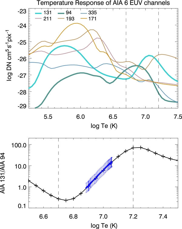
Figure 11. Top: temperature response curves of the AIA six EUV channels. Bottom: the ratio of the temperature response function of AIA 131 to 94 Å. Flux ratios estimated for the SA region during the flare and error bars indicating instrumental uncertainty of AIA are overplotted in blue. Vertical dashed lines show the temperature extent of the SA region, constrained by observations of the six EUV channels.
Download figure:
Standard image High-resolution imageThe white box shown in Figure 10 indicates the SA source area where we estimated the plasma temperature. The DN for the SA area was averaged and a background was subtracted. Considering that the SA location is in the corona, the background DN was found at a diffuse and stable emission region existing in the off-limb corona. We note that diffraction patterns, observed in AIA 131 Å (see Figure 3(c) in particular), caused by the bright flare loops contribute to the flux in the SA region. The measured contribution of diffraction patterns was found to be around 11% of the total DN of the SA area, so it is insignificant for these estimations (C. L. Raftery 2012, private communication). The bottom panel of Figure 11 shows the DN ratios of AIA 131 Å to 94 Å for the SA area (blue line). It is superposed on the ratio of temperature response curves of these two filters (black line). Using the GOES widget, we derived the temperature for the FL (White et al. 2005). Figure 12 shows the time variation of estimated plasma temperature for both regions, the FA (dotted line) and the SA (solid line). The FA temperature peaks at 18 MK at 23:56 UT and quickly decreases to 14 MK within 4 minutes. After that, it gradually decreases down to 8 MK. On the other hand, the SA temperature shows a steep increase around 10 MK until 23:57 UT but, during the decay phase, it seems to increase steadily until 00:10 UT and then decrease to 8 MK at 00:50 UT. Since the steady increase of the temperature takes place within given error bars, it may not be a real increase. However, it sustains its high temperature above 10 MK until 00:16 UT.
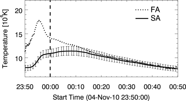
Figure 12. Time profiles of estimated plasma temperature of the flare-arcade (FA) and the supra-arcade (SA) structure with an estimation of error owing to the instrumental uncertainty of the AIA. The vertical dashed line at 00:00 UT indicates the time when the thermal free–free emission start to be dominant (see Figures 1 and 8). The physical parameters in Figure 13 have been derived from this time.
Download figure:
Standard image High-resolution image3.2. Emission Measure and Electron Density
The microwave emission, unlike EUV and X-rays, is little sensitive to the variation of the plasma temperature (see Equations (2) and (3)). Thus, it is appropriate to derive the emission measure of the plasma using the microwave emission during the phase when the plasma shows a clear temperature gradient. From the brightness temperature observed by NoRH at 17 GHz, we have derived the emission measure (EM) and electron number density (Ne) of the FA and the SA, during the decay phase, for the period from 00:00 UT to 00:50. Based on the observations, we assume that the microwave comes from the optically thin (τν ≪ 1) and thermal free–free emission of plasma. Thus, the relation between brightness temperature (TB) at specific radio frequency (ν) and plasma temperature (T) is described as (Dulk 1985):

where τν is
where the coulomb logarithm ln Λ = ln [4.7 × 10¹⁰(T/ν)]. T is a plasma temperature calculated in Section 3.1 and TB is obtained at ν = 17 GHz. The density of each sources can be derived from EM,
where zmeas is the averaged depth of the line of sight and f is the line of sight filling factor, f = zreal/zmeas (Dere 1982). The line of sight depth of the soft X-ray sources is assumed to be equal to the source width, zFA ≈ 23 Mm and zSA ≈ 40 Mm, respectively. It is difficult to determine the filling factors of observed loops or structures since present observations cannot resolve whether the plasma are filled uniformly or sparsely with separate multiple loops/structures. Dere et al. (1979), Dere (1982), and Tripathi et al. (2009) compared the density determined from the emission measure within the volume of interest with the density determined from two density sensitive spectral lines, establishing the filling factor within the source. The filling factor near unity was found by Dere et al. (1979) for solar flares and by Dere (1982) for two active region coronal loops. On the other hand, there seems to be evidence of filling factors as low as 5 × 10⁻² (Cargill & Klimchuk 1997). Recently, Tripathi et al. (2009) found that the filling factor increased with projected height of the hot coronal loops and was close to unity just beyond 40 Mm. In this analysis, we assume that the inner part of the FL and the SA is filled with plasma, and the electron number density along the line of sight is uniform, e.g., f ∼ 1.
Figure 13 shows the derived EM (top) and Ne (middle) for the FA and the SA with time. EM and Ne of the FA decrease constantly from 1.0 × 1030 to 0.2 × 1030 cm−5 and 2.0 × 10¹⁰ to 1.0 × 1010 cm−3, respectively. Contrary to this, EM and Ne of the SA increase from 0.2 × 1029 to 1.0 × 1029 cm−5 and from 2.0 × 10⁹ to 5.0 × 109 cm−3, respectively. The decreasing rate of Ne in the FA was 2.7 × 106 cm−3 s−1 throughout. On the other hand, the increasing rate of Ne of the SA was 1 × 106 cm−3 s−1 around the start of the decay phase and then gradually decreases to 1 × 105 cm−3 s−1 at the end of the flare. Based on the assumed z and calculated source area A, the total number of electrons decreased by 2.4 × 1034 s−1 for the FA and increased by 6.3 × 1034 s−1 around the start of the decay phase and 0.6 × 1034 s−1 at the end of the flare for the SA. Taking into account the increasing Ne and T in the SA, one can deduce that there is an injection of hot plasma into the SA from below.

Figure 13. Time profile of derived emission measure (top), electron number density (middle), and thermal energy (bottom) of the flare arcade (FA) and the supra-arcade (SA) structure during the decay phase. The error bars show the uncertainty of the temperature in Figure 12.
Download figure:
Standard image High-resolution imageFor consistency, we compare our estimates of temperature and emission measure with observations from RHESSI. A spatially integrated spectrum for the time interval 00:10:00 to 00:13:30 UT, taken immediately after spacecraft night, reveals a thermal spectrum with a temperature of 14 MK and an emission measure of 0.142 × 1049cm−3 for the combined FA and SA source contributions. However, due to low counting statistics, it is not possible to perform imaging spectroscopy to determine independent values of temperature and emission measure of the SA source. Nevertheless, we attempt to compare the flux ratio of the SA and FA that we would expect to see from RHESSI imaging observations given the temperature and emission measure estimates found using AIA and GOES. Using values obtained from AIA and GOES, and assuming isothermal free–free emission, we calculated the flux ratio of the FA and the SA sources, i.e., FFA: FSA, that we would expect to observe in the soft X-ray range observed by RHESSI (blue lines, Figure 14). This was done using the solarsoft routine f_vth.pro, which determines the expected radiation as a function of energy. The function contains a contribution from the optically thin thermal free–free bremsstrahlung and free-bound continuum, and line emission, primarily from highly ionized iron (seen in RHESSI spectra at 6.7 keV and 8 keV), obtained using CHIANTI. The continuum emission takes the form I( ) ≈ (EM/T1/2)exp (− /kBT), where is photon energy and kB is the Boltzmann constant. We then compared these values with those found from actual observations (red lines, Figure 14). We chose to make this comparison at 8 keV, where there were enough soft X-ray counts to reconstruct a RHESSI image over a narrow energy range. The calculations were done using the integrated time intervals required for RHESSI imaging. In general, the results are consistent with RHESSI observations. However, we note that the main source of error in these measurements comes from determining the source area of the SA, which is particularly difficult given its diffuse nature and intensity with respect to the compact source. We expect our source area to be accurate to around a factor of two; however, we note that it is possible that the source contains small- scale structure that cannot be reconstructed using this method.

Figure 14. Plot of the flux ratio between the FA and SA sources (FFA: FSA) for isothermal free–free emission at 8 keV. The blue lines show the expected ratio using temperature and emission measure estimates from AIA, GOES, and NoRH. Red lines show the flux ratio observed by RHESSI.
Download figure:
Standard image High-resolution image3.3. Thermal Energy
The thermal energy of the emitting plasma in the volume (Vmeas), which is determined by a source area of A multiplied by the assumed line of sight depth of zmeas (see Section 3.2), is given by

The filling factor is assumed to be unity (see Section 3.2). The bottom panel of Figure 13 shows the estimated thermal energy for both sources. Eth of the FA gradually decreases from 1.5 × 1030 erg at 00:00 UT to 0.4 × 1030 erg at 00:50 UT, while Eth of the SA increases from 0.5 × 1030 erg at 00:00 UT to 1.0 × 1030 erg at 00:16 UT and then sustains this value until 00:50 UT. To determine a time scale for the energy loss, cooling processes by radiation and conduction are considered. Using an estimate of loop radius from AIA 131 Å images, L = 29 Mm for the FL and 89 Mm for the SA, we found that the predominant cooling process is conduction and the estimated cooling time scale ( ) is 230 s for the FA and 390 s for the SA. However, considering the decreasing rate of the estimated temperature during the decay phase, the cooling time of the top of the FA down to 1 MK is 6400 s. Furthermore, the SA structure shows not cooling but heating for a while in the early part of the decay phase. Thus, it clearly shows that the significant energy injection took place in the FA and the SA during the flare decay phase.
4. SUMMARY AND DISCUSSION
We have examined the FA and the SA structure of M-class limb flare in morphology and physical parameters using multi-wavelength data. During the impulsive phase, it looks to be consistent with typical flares in several aspects: expansion of a bulk of plasma into the high corona, flare loops, and gyrosynchrotron emission due to electron acceleration. During the decay phase, the flare loops showed expansion, cooling, and decrease of emission as a consequent progress on typical flares, whereas the hot SA structure showed characteristic phenomena such as upflows of hot plasma and gradually increasing microwave emission at 17 and 34 GHz. The unique data set of high- resolution microwave, EUV, and X-ray data revealed details and interesting properties of the SA structure that seem to relate to the FA in which unresolved energy release processes might take place.
The multi-channel observations of microwaves and EUV gave us an opportunity to estimate the physical parameters of the SA structure and the FA. We found an increase in the plasma density within the SA structure (ΔNe ∼ 3.0 × 109 cm−3) during the decay phase and an increase of the thermal energy (ΔEth ∼ 4.5 × 1029 erg) at the early stage of the decay phase, whereas the FA showed a continuous decrease in the plasma density (ΔNe ∼ −1.0 × 1010 cm−3) and the thermal energy (ΔEth ∼ −9.0 × 1029 erg) during the decay phase throughout. One can speculate that increased energy in the SA structure is originated in-situ or above it. But, in the AIA EUV observations, there was no manifestation of hot plasma injection from higher altitudes above the SA structure, whereas there were upflows along a large-sized coronal loop. Thus, the origin of the energy above the SA structure is excluded from consideration. On the other hand, taking notice of the density and energy variation, the plasma that escaped from the flare loop-top might directly contribute to the increase of plasma in the SA structure. Considering these results, we propose two distinct scenarios for the hot plasma/energy source of the SA structure: (1) in-situ source and (2) FA.
The in-situ energy source for the SA structure can be a current sheet (here after CS) and a magnetic reconnection process in the CS. The hot plasma, such as observed SA diffuse structure, can be formed by the thermal conduction in the CS (see Yokoyama & Shibata 1997; Reeves et al. 2010; Reeves & Golub 2011). Figure 15(b) shows Scenario A with the CS and the magnetic reconnection process as a hot plasma/energy source of the SA structure, based on the standard flare model (see Forbes & Acton 1996). The anti-parallel magnetic fields surrounding the CS reconnect, and then reorganized fields retract along the direction in which the magnetic tension force acts, upward and downward (thick arrows). As a result, they come into view as upflows pushed by upward new fields and as the hot source on the SA by an interaction with downward fields. So far, SA structures have been interpreted as a consequence of a current sheet based on the standard model with the following manifestations: SADs (McKenzie & Hudson 1999; McKenzie & Savage 2000), continuously rising X-ray sources in the SA (Gallagher et al. 2002), inflows and outflows near the current-sheet (Yokoyama et al. 2001; Savage et al. 2010, 2012), and the hot diffuse plasma (Yokoyama & Shibata 1997; Reeves et al. 2010). These points are crucial evidence for identifying the flare dynamics in the standard model and with our event. On the other hand, we found that upflows streamed along large curvature and large coronal loops. In Scenario A, the current sheet is formed by upward expansion of the flux rope system so that most upflows from it should have a similar trajectory toward the flux rope system. Thus, it is necessary to consider the upflows with another mechanism as well, as a result of magnetic reconnection.

Figure 15. Illustration of the flare during the decay phase. (a) Observed features with possible coronal magnetic structures. (b) Scenario A and (c) scenario B with three steps for the formation of the thermal supra-arcade structure.
Download figure:
Standard image High-resolution image
Though the FA is a major source of energy during the flare, it does not play any role for the SA structure in Scenario A. Thus, we propose another scenario where the FA is deemed as a hot plasma/energy source of the SA structure. Considering observed features summarized in Figure 15(a), we believe that there are overlying closed magnetic loops which extend into the high corona above the flare region during the decay phase. Figure 15(c) shows the same picture seen from a different angle, with a description of one possible scenario, Scenario B, where hot plasma and energy supply are originated from the FA. The SA structure consists of three closed magnetic loops: two large-sized loops and one thick loop. Both legs of the thick loop are rooted on the same active region as the flare, while the two large-sized loops have only one leg rooted on the active region. Due to the energy release process caused by magnetic reconnection or by an instability in the FA (that may occur but cannot be resolved by current observations), hot plasma is ejected from it, mostly from the top, and injected into the three ambient loops. This results in upflows along the two large-sized loops. Meanwhile, the thick loop has a particular shape as follows: broad width near the top and thin legs below. The hot plasma is injected into both legs of the thick loop and then goes up along it. Continuously injected hot plasma piles up in the upper part of the thick loop and results in an increase of the plasma density.
One possible mechanism for the generation of hot plasma below the SA structure is the magnetic reconnection triggered by loop–loop interaction (Canfield & Reardon 1998; Moore et al. 2001) or interchange reconnection between the emerging flux and pre-existing field (Heyvaerts et al. 1977; Shimojo & Shibata 2000). This could generate hot plasma by chromospheric evaporation and fill out the flare loops. This typically involves a change of the field morphology and/or outflows, such as a jet which occurs abruptly and ceases quickly. But, we found a quite stable FA without recognizable field change during the decay phase in six EUV-channels of the AIA. Thus, it might take place during the impulsive phase of the flare when images of the flaring region were saturated but it is hard to say that there was some change of the coronal field morphology during the decay phase which can demonstrate possibilities mentioned above.
Offering a different view point from magnetic reconnection, Gary (2001) have suggested that "pressure forces might drive some dynamic loops without having major magnetic reconnection or global magnetic field changes." In a concrete way, Shibasaki (2001) suggested that the disruption on the apex of the flare loop-top occurs by localized interchange instability, so called "ballooning instability." This instability, in turn, generates various elements associated with the solar flare, including plasma ejection, turbulence, high-energy particle acceleration, and so on (Zaitsev & Stepanov 1985; Hood 1986; Shibasaki 2001). In curved coronal loops, the balance of upward (pressure gradient, magnetic pressure gradient, and centrifugal force) and downward forces (magnetic tension and gravity force) establish stable loop structure. If the loops become unstable by upward centrifugal force owing to the thermal motion of plasma, then we can expect localized interchange instability at the apex of the loops (see Shibasaki 2001). Assuming the thermal motion in flare loops consisting of the FA and applying obtained physical conditions of T ∼ 10 MK and R ∼ 23 Mm into Shibasaki's (2001) formula, one can find that the upper boundary of the flare loops easily suffers instability toward the high corona. It can cause disruption allowing the plasma to cross the magnetic field of the flare loops so that the hot plasma on the top of the flare loops escapes upward high in the corona. If disruption happens in each loop in the arcade successively, continuous plasma ejection can be explained.
In order to trigger the ballooning instability, finite plasma β (the ratio of plasma pressure to magnetic pressure), which can break MHD equilibrium, is essential. We went through the circular polarization degree (rc) using intensity and polarization maps from NoRH 17 GHz and found that rc was not over ∣0.1∣ % in the FA. This implies that the magnetic field strength of the flare loops comprising the FA is considerably weak (Dulk 1985). For a homogeneous, thermal, and optically thin plasma, a net polarization degree rc is equal to 2 cos θνB/ν, where θ is the angle between the line of sight and magnetic field line and νB is the electron–cyclotron frequency, 2.8 × 10⁶B (see Bogod & Gelfreikh 1980). Assuming that the FA consists of well-aligned flare loops and θ on the top of the flare loops has inclination in the range of θ = 75° ∼ 85°, the magnetic field strength is estimated in the range of 12 to 35 gauss. Based on the results of physical parameters of FA, Ne = 1010 cm−3 and T ∼ 107 K, the thermal pressure of plasma, 2NekbT, is obtained. Thus, plasma β is estimated in the range of 0.6–5, and this finite plasma β is enough to trigger the ballooning instability, particularly near the top of the flare loop where the minimum field strength in the bipolar flare loop is expected (Shibasaki 2001). Taking many strands of the flare loops into consideration, this instability can continue as long as the flare loops satisfy the above conditions. However, since it arises abruptly in a tiny segment, the direct moment of disruption in the top of the flare loops is hard to catch with present instruments.
The ballooning instability is one of a promising candidate of plasma disruption in Tokamak experiments (Park et al. 1995; Cowley et al. 1995; Fredrickson et al. 1996). It usually occurs near the β limit, so called high-β disruption. The MHD theory predicts that the nonlinear ballooning instability and total kinetic energy of the plasma grows explosively in a localized narrow region (Hurricane et al. 1997; Cowley et al. 2003; Zhu et al. 2009). However, consequences of the nonlinear ballooning instability and how the energy is actually transported has defied the theory. Its explosive manner and energy loss are quite similar to solar flares and magnetospheric substorms, despite huge variations in size and plasma parameters (see Hurricane et al. 1997). Thus, we consider that the ballooning instability is capable of transporting confined plasma across the field and resulting in solar flares.
In this study, we have examined the morphological evolution and overall physical parameters of the SA structure and flare loops. The results show that it is more than likely that the flare loops were formed by the reconnection in high corona as a typical standard picture, but the SA structure is not fully elucidated by it. Thus, we propose ballooning instability as an alternative to the standard picture. However, it should be proved by a precise estimation of magnetic field strength in the flare loop. The chromospheric and/or low atmospheric energy source for the hot flare loops is also an important issue which needs to be further studied with detailed observations. As for the analysis of the number density and thermal energy of the plasma, one should notice that it could involve a substantial uncertainty from the assumption of the line-of-sight depth and, hence, the volume. This limitation arises because the data has projected information. This work is significant in expanding our insight and understanding of the solar flare, particularly for the gradual phase of the flare. Future work should be done to find more events for microwave SA structure constituted of flare plasma and study the statistical properties.
The authors sincerely appreciate the anonymous referee for the constructive comment. We thank Drs. Nakajima, Raftery, and Reznikova for their worthy contribution and Dr. Reeves for providing us calibrated AIA data at the beginning of the study. This research was supported by the Basic Science Research Program through the National Research Foundation (NRF) of Korea Grant funded by the Korean Government (NRF-2013M1A3A3A02042232) and the NRF of Korea Grant funded by the Ministry of Education (NRF-2013R1A1A2058409). The AIA data have been used courtesy of NASA/SDO and the AIA, EVE, and HMI science teams. RHESSI is a NASA Small Explorer Mission.