


ABSTRACT
In two previous papers, we presented a global model for the analysis of magnetic clouds (MCs), where the three components of the magnetic field were fitted to the corresponding Geocentric Solar Ecliptic experimental data, obtaining reliable information, for example, about the orientation of these events in the interplanetary medium. That model, due to its non-force-free character, (∇p ≠ 0), could be extended to determine the plasma behavior. In the present work, we develop that extension, now including the plasma behavior inside the cloud through the analysis of the plasma pressure, and define a fitting procedure where the pressure and the magnetic field components are fitted simultaneously. After deducing the magnetic field topology and the current density components of the model, we calculate the expression of the pressure tensor and, in particular, its trace. In light of the results, we conclude that incorporating the plasma behavior in the analysis of the MCs can give us a better scenario in which to understand the physical mechanisms involved in the evolution of such magnetic structures in the interplanetary medium.
Export citation and abstract BibTeX RIS
1. INTRODUCTION
Magnetic clouds (MCs) are one of the most interesting and studied phenomenon that are a subset of the interplanetary coronal mass ejections (ICMEs), which are solar transient events coming from the Sun surface. These correspond to phenomena that are one of the main results of geomagnetic storms, and their implication in the space weather forecast and, therefore, also in space technology development is relevant. From the large number of studies undertaken up until now, first from in situ observations and more recently from remote sensing measurements, we are aware that they are structured and ordered magnetic field topologies.
Burlaga et al. (1981) were the first to establish the concept of MCs from the experimental data, basing them in measurements of the magnetic field and solar wind plasma data. Most of the time they were followed by an interplanetary shock, showing a smooth rotation of the magnetic field and a relatively high magnetic field strength over the usual values of the solar wind and low-β plasma; even more recently, the presence of bi-directional electrons and the unusual charge states of oxygen and iron have been added.
On the other hand, there are many ICMEs that correspond to magnetic structures coming from the Sun that do not clearly show all these requirements. They are called ejecta (EJs). Then, an important global question has arisen about the topology of all of these phenomena concerning their flux-rope magnetic field configuration. Thus, although the phenomenon of MCs is considered to be a well-defined magnetic field topology, the nature and structure of the EJs are still an open question (Hidalgo et al. 2013). That fact was the origin of the workshop "Living with a Star Coordinated Data Analysis Workshop: Do All CMEs Have Flux Rope Structure?" first held in San Diego in 2010 September. The second workshop was held in Alcalá de Henares (Spain), in 2011 September (Gopalswamy et al. 2013). Different models and techniques have appeared in the literature to analyze the physics of MCs, all of which with the goal of understanding the global structure, the initiation and connection with the Sun, their interactions with the solar wind along its movement in the interplanetary medium, and, finally, their effect on the Earth's magnetosphere. All those models use one of two ways to focus on the problem: on one hand, from the remote sensing point of view looking at the Sun surface, and, on the other hand, analyzing in situ measurements at 1 AU in light of analytical models and numerical simulations. We utilized the latter.
Goldstein (1983) proposed a topology of MCs, similar to that described by the Burlaga criteria, based in a flux-rope picture with a force-free character, summarized in the equation  , i.e.,
  . Lundquist (1950) found static axially symmetric magnetic field solutions of this equation in cylindrical geometry, all of which depend on the zeroth- and first-order Bessel functions. In general, most of the studies with this focus have restricted their attention to the case where the parameter α is constant. However, the main consequence of the plasma behavior of this magnetic topology assumption is summarized in the equation ∇p = 0, i.e., the pressure is constant inside the MC time interval. However, looking at the pressure data of any MC, some structure in the associated data is clearly observed, although at a magnitude much lower than the corresponding values in the forward shocks of these events.
Analytical models for their topology, not only for the cross section but also for the global structure of the MC, have been proposed in the literature, some of them without imposing the force-free restriction. However, the relaxation of such force-free conditions is necessary in order to understand in a more appropriate scenario the evolution of the MC structures in the interplanetary medium and in particular their expansion. Even more, the inclusion of the plasma pressure can allow us to analyze the MC interaction with the solar wind and their effects on the magnetic field of the magnetosphere.
On the other hand, until now, it is possible to find various numerical models in the literature, which also try to determine the dynamical evolutionary processes and mechanisms of the CMEs in the interplanetary medium and their interactions. Simultaneously, the remote sensing observations have allowed us to develop techniques to visualize the three-dimensional CME structure, mainly due to the STEREO mission, although such techniques only provide information about geometrical features of CMEs without analyzing the physical mechanisms that are carried out in the MCs evolution and propagation.
The present work is the next step in the development of a more reliable analytical model for the global magnetic topology of MCs which has recently begun with two previous works (Hidalgo & Nieves-Chinchilla 2012; Hidalgo 2013). We assumed toroidal shape for the global topology of the MCs but supposed that they have non-uniform cross sections. Establishing an intrinsic coordinate system (associated with that topology), we solved the Maxwell equations in an appropriated framework to focus the problem and calculated the expressions not only for the magnetic field components, even in the GSE coordinate system (directly comparable with the corresponding magnetic field components as obtained by the spacecrafts), but also for the expressions of the current density. In the present work, from the components of both physical magnitudes, we calculate the plasma pressure tensor.
The paper is organized as follows. In Section 2, the determination of the trace of the pressure tensor is presented in detail. Section 3 is devoted to explaining the procedure used to fit the model to the experimental data. The data studied and fitted are described in Section 4; they are related to 12 events, showing different behavior in the plasma pressure data. Finally, in Section 5, a summary and discussion section describes the results obtained with the model for the selected MCs.
2. THE MODEL
In spite of the several published models for understanding the physics of MCs, one open problem still remains: the inclusion of the behavior of the plasma in their global analysis. As we have mentioned above, the model by Burlaga (Burlaga et al. 1981; Lepping et al. 1997) implies a constant pressure inside the MC due to its force-free character, in contradiction with the experimental observations, that show, although smaller in magnitude than the values seen in the forward shock or the back shock, a clear structure inside MCs (see Figures 2–13).
Osherovich et al. (1993, 1995) were the first to try to understand the behavior of the plasma by incorporating it in their analysis of MCs, although their analytical model has a pure theoretical character and cannot be fitted to the experimental data. More recent studies have also included this kind of analysis, although they were included from the numerical and/or simulation point of view (for example, Hu & Sonnerup 2002).
In the present work, we continue with the development of our analytical global model (Hidalgo & Nieves-Chinchilla 2012; Hidalgo 2013). We chose the appropriate intrinsic coordinates to treat the topology assumed for the MCs: a toroidal coordinate system where the minus radius of the torus varies along it. In Figure 1, we give an overview of this global geometry as it is assumed in the model (to draw the figure we have used pictures from the STEREO Web site: http://stereo-ssc.nascom.nasa.gov/where/)—a more detailed description about the topology and the corresponding coordinate system can be found in Hidalgo & Nieves-Chinchilla (2012). Then, from the Maxwell equations for the magnetic field and the continuity equation, we can obtain analytical expressions for the magnetic field vector,  , and the plasma current density,
  , assuming for this last magnitude that there are stationary conditions for the charge density of electrons and protons, i.e.,∂(ρe + ρp)/∂t = 0, at the timescale we are interested in for the evolution of the cloud. The current density is given as
  , where
  and
and  correspond to the electron and proton current densities, respectively, and its components, as it is deduced from the plasma continuity equation, are
for the poloidal component and
for the axial component. The terms α and λ are constants, parameters of the model. These current density components and the magnetic field components have been described in detail in previous papers (Hidalgo & Nieves-Chinchilla 2012; Hidalgo 2013); in these versions of the model only the magnetic field components are developed and, although the current density is also obtained, the plasma behavior of the MCs is not included in the procedure and analysis.
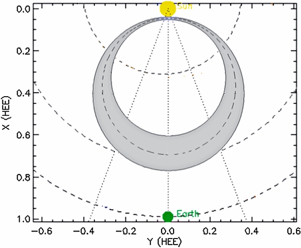
Figure 1. Overview of the global geometry of the MCs as is assumed in the model (to draw the figure, we have used pictures from the STEREO Web site: http://stereo-ssc.nascom.nasa.gov/where/). HEE: Heliocentric Earth Ecliptic coordinates.
Download figure:
Standard image High-resolution imageWe now determine the theoretical expressions of the plasma pressure with the aim of including it in the fitting procedure of the model to the experimental data. Our starting point for that task will be the force equation, given by
for every particle species, where n is the corresponding particle density, q = ±e is the charge, and m is the mass. The topology assumed for the MCs provide a tensor character to the plasma pressure, , which is diagonal if it is deduced in the intrinsic toroidal coordinate system.
We need, of course, some assumptions to obtain an analytical expression from Equation (3). Considering the timescale of the evolution of the cross section of the cloud and the linear decrease of the velocity associated with the expansion of it, we establish the following hypothesis on the kinematics of the plasma in the cross-section of the MCs:
If we added Equations (3), one corresponding with protons and the other with electrons, we obtain

where  is the total pressure tensor associated with both species inside the cloud, and j given by Equations (1) and (2), and the magnetic field components are those determined in Hidalgo & Nieves-Chinchilla (2012) and Hidalgo (2013).
Solving Equation (5), we can determine the components of the diagonal pressure tensor. They are

where ρ0 is the mean radius of the torus; and  is the axial magnetic field at the axis of the torus, imposing
  to be constant. Moreover, on one hand, considering magnetic flux conservation along the torus, we will express the poloidal magnetic field integration constant as
  , where
  depends on r. The term
  corresponds to the Heaviside function. To be able to use the analytical expressions, we must make a hypothesis about the behavior of the auxiliary function f(ψ), which, as in previous works, we assume upon first approach to be f(ψ) = Csin(ψ/2), C being an adjustable constant (at zero the torus would have a uniform cross-section).
  ,
,  , and
, and  are constant terms associated with each pressure component.
From Equations (6)–(8), we calculate the trace of the plasma pressure tensor that will be the magnitude we will introduce in the fitting procedure,

In order to maintain the neutrality of the plasma, we assume that it is similar for both main species: electrons and protons.
3. PROCEDURE
In the procedure, we simultaneously fit the theoretical GSE magnetic field components and the trace of the pressure tensor of this global model and the corresponding experimental measurements, and then minimized the function
where N is the number of experimental points, Tr(p) is the trace of the hydrostatic pressure, Bexp is the experimental data of the GSE components of the magnetic field, and BGSE is the corresponding theoretical expressions (Hidalgo & Nieves-Chinchilla 2012). The constants pn = 10−12 Pa and Bn = 10−9 T have been introduced to make every magnitude included in the fitting process comparable and to provide a dimensionless χ2 function.
Because of the high value of the x-GSE component of the solar wind velocity in the MCs intervals, we can consider the path of the spacecraft parallel to the x-GSE direction. Taking into account the mean solar wind velocity in the cloud interval, 〈vsw〉, and all the parameters related to the orientation of the cloud (the attitude of the axis of the MC, the latitude, θ, and the longitude, ϕ, and the minimum distance between the spacecraft path and its axis, y0), we can determine the theoretical local magnetic field components in the GSE system. Moreover, also the coordinates rspc(t), φspc(t), and ψspc(t) of the spacecraft at any time t inside the MC. Now, introducing the trace of the pressure tensor in the fitting procedure involves one more parameter with respect to those of our previous work (Hidalgo 2013): the constant parameter related to the pressure, p0.
Finally, in all the fitting processes of the events considered, measured by the spacecrafts at 1 AU, we have fixed a mean radius of the torus, ρ0, of 0.5 AU.
Therefore, fitting the model, we obtain not only the magnetic field components but also the plasma pressure.
4. DATA
During the two meetings of the workshop "Living with a Star Coordinated Data Analysis Workshop: Do All CMEs Have Flux Rope Structure?"—the first in San Diego, CA (USA, 2010) and the second one in Alcalá de Henares (Spain, 2011)—59 ICMEs events in the time period 1997–2006 were selected and analyzed. Of those, 24 were unambiguously associated with MCs, i.e., the times series of the magnetic field components and the plasma measurements follow the criteria and signatures established more than 30 yr ago by Burlaga et al. (1981). The remaining events, the so-called EJs—a proportion of around two-thirds of all events—do not present as clear of signatures, and we cannot be aware of their flux-rope topology. The only way to elucidate this question is to fit a flux-rope model to the corresponding data and to draw conclusions about the presence of this kind of structure, basing it on the fits of the model to the data. More detailed information about the events mentioned above is included in the general analysis that can be found in the conference proceedings (Gopalswamy et al. 2013).
All the data and experimental information used in the present work come from the ISTP program and OMNIWeb.
Following the criteria defined by Burlaga et al. (1981), the plasma information used to establish the boundaries in all the events studied has been the plasma β. In Table 1, we detail the day of year (doy) for the boundaries of every event analyzed, in correspondence with the entrance/exit of the satellite in/of it, and the mean velocity at 1 AU used in our treatment.
Table 1. MC's Time Interval Used in the Analysis of the Events Selected in the Present Work
| Event | MC Interval | 〈vSW〉 |
|---|---|---|
| (yy-mm-dd) | (doy) | (km s−1) |
| 97-01-10 | 10.246→11.051 | 450 |
| 99-08-08 | 221.499→222.422 | 340 |
| 00-02-22 | 52.426→52.894 | 370 |
| 00-07-12a | 194.155→195.116 | 480 |
| 00-07-28 | 210.652→211.272 | 460 |
| 01-04-12a | 102.367→102.279 | 675 |
| 02-05-19 | 139.186→140.093 | 430 |
| 02-08-01 | 213.110→213.301 | 450 |
| 04-11-09 | 315.138→315.672 | 700 |
| 05-01-16a | 16.719→17.300 | 540 |
| 05-05-20 | 140.668→141.276 | 440 |
| 12-09-10 | 250.144→250.623 | 420 |
Note. The corresponding mean velocities, necessary for our fitting procedure, are also detailed. aEjecta with flux-rope structure (see the text for details).
Download table as: ASCIITypeset image
In all the MC figures that are given, the graphs presented are the magnetic field strength, B, the Cartesian GSE-components (Bx, By, Bz), the proton pressure, and the bulk solar wind velocity. The vertical dotted lines represent the time boundaries of the cloud following Burlaga's criteria. The toroidal model fittings results are also superimposed on the experimental data with solid lines for the strength, the three magnetic field components, and the pressure.
In the present study, we have selected 11 events from the list of the workshop mentioned above, 8 of which are MCs and 3 are EJs. The last additional event corresponds to the event of 2012 September, which is selected for the profile of its pressure behavior.
The analyzed events are as follows (formatted as yyyymmdd): MC 19970110 (Figure 2), MC 19990808 (Figure 3), EJ 20000712 (Figure 4), EJ 20010412 (Figure 5), MC 20020519 (Figure 6), MC 20050520 (Figure 7), MC 20000222 (Figure 8), MC 20000728 (Figure 9), MC 20020801 (Figure 10), EJ 20050116 (Figure 11), MC 20041109 (Figure 12), and MC 20120910 (Figure 13).
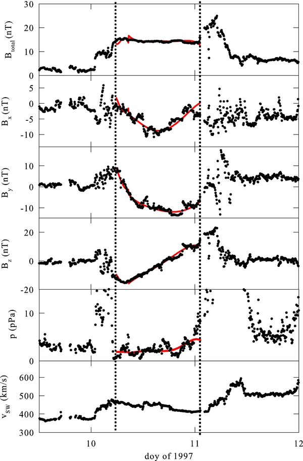
Figure 2. Data from OMNIWeb for the magnetic cloud of 1997 January, and the results of the global model for the magnetic field strength, B, the Cartesian GSE-components (Bx, By, Bz) and the proton pressure. The bulk solar wind velocity is also shown. The vertical dotted lines represent the time boundaries of the cloud as chosen following Burlaga's criteria, using the β-plasma. Superimposed on the experimental data, the toroidal model predictions are shown with solid lines (see the text for details).
Download figure:
Standard image High-resolution image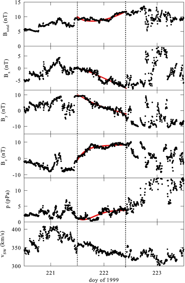
Figure 3. Same graphs as in Figure 2 for the magnetic cloud of 1999 August.
Download figure:
Standard image High-resolution image
Figure 4. Same graphs as in Figure 2 for the flux rope structured ejecta of 2000 July 12.
Download figure:
Standard image High-resolution image
Figure 5. Same graphs as in Figure 2 for the flux rope structured ejecta of 2001 April.
Download figure:
Standard image High-resolution image
Figure 6. Same graphs as in Figure 2 for the magnetic cloud of 2002 May.
Download figure:
Standard image High-resolution image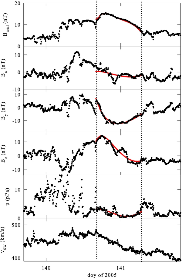
Figure 7. Same graphs as in Figure 2 for the magnetic cloud of 2005 May.
Download figure:
Standard image High-resolution image
Figure 8. Same graphs as in Figure 2 for the magnetic cloud of 2000 February.
Download figure:
Standard image High-resolution image
Figure 9. Same graphs as in Figure 2 for the magnetic cloud of 2000 July 28.
Download figure:
Standard image High-resolution image
Figure 10. Same graphs as in Figure 2 for the magnetic cloud of 2002 August.
Download figure:
Standard image High-resolution image
Figure 11. Same graphs as in Figure 2 for the flux rope structured ejecta of 2005 January.
Download figure:
Standard image High-resolution image
Figure 12. Same graphs as in Figure 2 for the magnetic cloud of 2004 November.
Download figure:
Standard image High-resolution image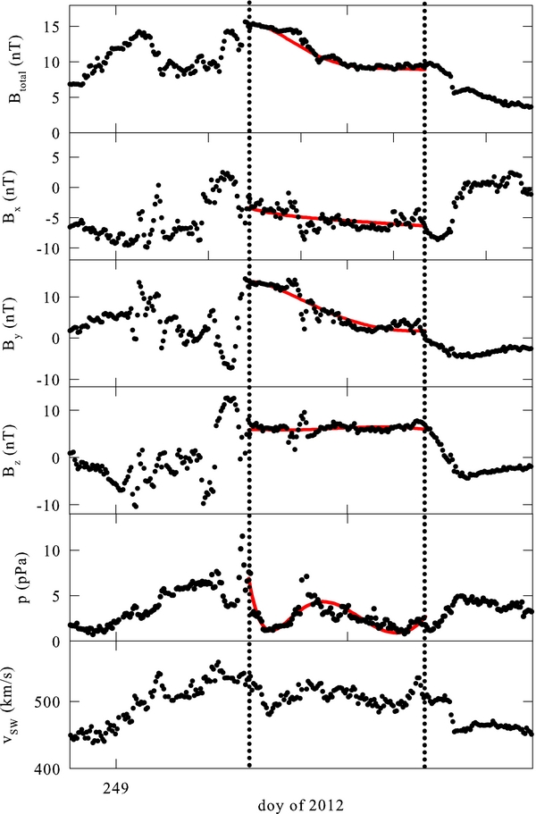
Figure 13. Same graphs as in Figure 2 for the magnetic cloud of 2012 September.
Download figure:
Standard image High-resolution image
Although in all the selected MC events several different shapes in the magnetic field components are present, the pressure data exhibit quite similar behavior; it is similar even in the EJ events considered (see below).
5. SUMMARY AND DISCUSSION
The two main features of the analytical model presented is, first, the assumption of a flux-rope topology and, second, its non-force-free character. This last condition implies a non-constant pressure behavior inside the MC. Concerning the topology, we suppose a torus structure with a maximum variable radius cross section along it, and with a circular cross-section. In order to get analytical expressions to compare directly with the experimental data, we have also assumed the condition of a very large mean radius of the torus, i.e., ρ0≫.
Additionally, the model includes the expansion of the cross section of the MC, for which we assume a time linear dependence in all the components of the plasma current density, i.e., proportional to (t0 − t), where t is the time variable, (in our analysis it will correspond to the time of the passage of the spacecraft through the cloud, considering t = 0 at the entrance of it). t0 is a time parameter characterizing the expansion of the cloud. (The time dependence of physical magnitudes must be linear in order for our model to be physically consistent (Hidalgo & Nieves-Chinchilla 2012). On the other hand, the analytical expression for the pressure used to fit the model to the experimental data is the trace of the pressure, Equation (9).
The parameters of the model related to the orientation obtained from the fitting, taking into account not only the magnetic field components but also the trace of the plasma pressure, are the same as achieving the fitting only considering the magnetic field components. However, we find an improvement in incorporating the plasma pressure in the treatment: the reduction in the dependencies associated with the plasma behavior parameters (in particular those related to the current density).
In all of the MC figures shown in the present work, superimposed onto the experimental data, averaged over five minutes, the model predictions are represented with solid lines.
In all the events, the plasma pressure shows a structure, i.e., they cannot be considered as a constant. For the sake of clarity, we have grouped them as a function of the similar shape of this magnitude: Then, we have the behavior shown by the MCs shown in Figures 2 and 3 and where the pressure increases toward the back of both events. On the other hand, the plasma pressure in Figures 4–7 presents a maximum inside the MC close to the forward shock, decreasing progressively until its back part. Figures 8–11 present a maximum in the behavior of the pressure in the middle part inside the MC. Finally, in Figures 12 and 13, we can observe a more complex structure with higher values in the region close to the forward shock of the MC and another maximum in the central region of them.
The quite good quality of the fittings, not only in the magnetic field components but also in the trace of the pressure, is clearly noted in all the selected cases shown here, leading us to conclude that the developed model, in a previous version only fitted to the magnetic field components and now incorporating the pressure, can be a potentially valuable approach to the magnetic topology and evolution of those phenomena at distances from Sun of the order of 1 AU. Moreover, the inclusion of the analysis of the pressure makes the model more consistent and, in light of the results, can be a good tool for understanding the physical mechanisms inside the MC as it evolves in the interplanetary medium.
Additionally, the analysis of the pressure can help to answer one of the open questions about the set of ICMEs called EJs: if their magnetic structure responds to a flux-rope topology. In the present study, we have incorporated three cases classified previously as EJ and analyzed them only fitting the magnetic field components: EJ 20000712 (Figure 4), EJ 20010412 (Figure 5), and EJ 20050116 (Figure 11; Hidalgo et al. 2013). In fact, as we see in the corresponding figures, they show similar behaviors in the plasma pressure as the MCs. (A more involved analysis of the EJ phenomena can be found in the reference given above (Hidalgo et al. 2013). The main conclusion of that paper was that those phenomena show worse definition in their signatures in the interplanetary data because the satellites passing through these events are close to the flank of the flux-rope structure.)
Therefore, our model is now capable of establishing the flux-rope character of the EJ in a more appropriate way, assuring the presence of this topology not only from the magnetic field profile but also from being helped by the plasma pressure, additionally allowing us to obtain more physical knowledge of the phenomenon, specifically about the attitude of the corresponding flux-rope structure (the latitude with respect to the ecliptic plane, θ, and the longitude in the ecliptic plane with respect to the Sun–Earth line, ϕ).
Moreover, incorporating the pressure of the MCs in the model opens the door to studies of the relationship between MCs and geomagnetic storms, i.e., the MCs plasma pressure influence over the magnetosphere and, in particular, their influence on the recovery phase of the geomagnetic storms.
The next step will be to include in the treatment the current density, although the main problem with this magnitude will be obtaining experimental data.
The author wishes to acknowledge data and information obtained from the ISTP program, OMNIWe, and the STEREOs (A and B) team, for permission to use pictures from its Web site. This work has been supported by the Comisión Interministerial de Ciencia y Tecnología (CICYT) of Spain. Project References: AYA2010-12439-E and AYA2011-29727-C02-01.