


ABSTRACT
To study the role of protosellar jets and outflows in the time evolution of the parent cores and the protostars, the astronomical community needs a large enough database of infrared images of protostars at the highest spatial resolution possible to reveal the details of their morphology. Spitzer provides unprecedented sensitivity in the infrared to study both the jet and outflow features, however, its spatial resolution is limited by its 0.85 m mirror. Here, we use a high-resolution deconvolution algorithm, "HiRes," to improve the visualization of spatial morphology by enhancing resolution (to subarcsecond levels in the IRAC bands) and removing the contaminating side lobes from bright sources in a sample of 89 protostellar objects. These reprocessed images are useful for detecting (1) wide-angle outflows seen in scattered light, (2) morphological details of H2 emission in jets and bow shocks, and (3) compact features in MIPS 24 μm images as protostar/disk and atomic/ionic line emission associated with the jets. The HiRes FITS image data of such a large homogeneous sample presented here will be useful to the community in studying these protostellar objects. To illustrate the utility of this HiRes sample, we show how the opening angle of the wide-angle outflows in 31 sources, all observed in the HiRes-processed Spitzer images, correlates with age. Our data suggest a power-law fit to opening angle versus age with an exponent of ∼0.32 and 0.02, respectively, for ages ⩽8000 yr and ⩾8000 yr.
Export citation and abstract BibTeX RIS
1. INTRODUCTION
Protostellar outflows and jets are believed to play a crucial role in determining the mass of the central protostar and its planet-forming disk by virtue of their ability to transport energy, mass, and momentum of the surrounding material and thus terminate the infall stage in star and disk formation. It is now well recognized that jets and outflows are essential and inherent to the star-formation process and play a key role in the structure and evolution of the molecular clouds in star-forming regions. The protostellar outflows are broadly classified into two types: molecular outflows traced mainly with CO emission and jets observed by optical line emission (cf. recent reviews by Arce et al. 2007; Bally 2007; Pudritz et al. 2007). Observations indicate that around some protostars, high-velocity jets with a narrow opening angles are enclosed by a low-velocity outflow with a wide opening angle (e.g., Mundt & Fried 1983; Velusamy et al. 2007, 2011), however, in others, only one component is observed. Poorly collimated flows can be due to extreme precession of the jet (Shepherd et al. 2000) and are indistinguishable from wide-angle outflows. The wide-angle outflows, which are also observed in the scattered light, are often missed in the optical or near-infrared due to instrument insensitivity to faint emission and confusion from the bright protostellar emission. Spitzer provides unprecedented sensitivity in the infrared to detect the jet/outflow features. IRAC, Infrared Spectrograph (IRS), and MIPS observations can provide new insights into the structure, morphology, and physical and chemical characteristics of the outflow sources as demonstrated, for example, in the observations of HH46/47 by Noriega-Crespo et al. (2004b) and Velusamy et al. (2007), Cep E by Noriega-Crespo et al. (2004a) and Velusamy et al. (2011), L1512F by Bourke et al. (2006), L1448 by Tobin et al. (2007) and Dionatos et al. (2009), L1251 by Lee et al. (2010), and HH211 by Dionatos et al. (2010). Using IRAC colors alone, Ybarra & Lada (2009) demonstrated the feasibility of studying the pure rotational H2 line emission in shocks without the need for spectroscopic data. To obtain the maximum information from the Spitzer images, Backus et al. (2005) and Velusamy et al. (2008) developed the deconvolution program HiRes and demonstrated that resolution-enhanced reprocessing of Spitzer images (Velusamy et al. 2007, 2011) brought out more clearly the morphologies of (1) wide-angle outflow cavities in the IRAC 3.6 and 4.5 μm images by scattered starlight, (2) jets and bow shocks in H2 molecular emission within the IRAC bands, and (3) the hottest atomic/ionic gas in the jet head characterized by [Fe ii] and [S i] line emission within the MIPS 24 μm band. However, to make further progress, we need a large sample of objects covering protostars of different mass and luminosity and evolutionary state.
In this paper, we present the deconvolved Spitzer IRAC and MIPS images of a large sample of 89 protostellar objects. These HiRes deconvolved images and FITS image data were developed under NASA's Astrophysics and Data Analysis Program for the purpose of making them available to the astronomical community for further studies of these protostellar objects. The use of resolution-enhanced (HiRes-deconvolved) Spitzer images to study the morphology and properties of the protostar and its jet outflow components has been illustrated in our earlier papers (Velusamy et al. 2007, 2011). It is not practical to discuss all the morphological details for the large sample of protostars, outflows, and jets presented here; instead, to highlight the rich detail in these HiRes images, we discuss the morphology of one outflow in L1527 to reinforce the fidelty of HiRes processing and overall benefits. In addition, to illustrate how such a large database can be useful, we use the opening angle of the wide-angle outflows in our sample to discuss the possible evolution of opening angle with age. One of the outstanding issues in protostellar evolution is the role played by outflows in regulating the protostellar mass accreting process. Outflows are effective in clearing the material from the core that feed the growth of the protostar (Arce & Sargent 2006) and a widening of the outflow cavity with age can lead to termination of the infall (Velusamy & Langer 1998). The large data set here shows further evidence for a widening opening angle with age.
2. Spitzer DATA AND ANALYSIS
It can be difficult to trace all the protostellar components, including the extended low surface brightness features associated with the outflow or jets, in the Spitzer mosaic images because these may be confused by the presence of side lobes (Airy rings) surrounding the high-brightness protostar and/or the disk. However, by applying the HiRes algorithm, one can minimize and at best remove the diffraction effects of the brightest features, thus enabling improved visualization of the low surface features around them. Furthermore, the resolution enhancement provides a sharper view of the outflow cavity walls, molecular jets, and bow shocks.
2.1. Selected Jets and Outflow Sources
The sample of Class 0 protostars, H2 jets, and outflow sources we selected for HiRes deconvolution of Spitzer images are listed in Table 1. The majority of our target protostellar objects were selected from "The Youngest Protostars" webpage hosted by the University of Kent (http://astro.kent.ac.uk/protostars/old/), which are based on the young Class 0 objects compiled by Froebrich (2005). In addition to these objects, our sample includes some Herbig-Haro (HH) sources and a few well known jet outflow sources. Our sample also includes one high-mass protostar (IRAS 20126+4104; cf. Caratti o Garatti et al. 2008) to demonstrate the use of HiRes for such sources. Our choice for target selection was primarily based on the availability of Spitzer images in IRAC and MIPS bands in the archives and the feasibility for reprocessing based on the published Spitzer images wherever available.
Table 1. List of Protostars, Jets, and Outflows in the Spitzer HiRes Processed Sample
| No. | Primary Name | Other/ | R.A. | Decl. | Ref | Dataa | Figure |
|---|---|---|---|---|---|---|---|
| Region | (2000) | (2000) | No. | ||||
| 1 | HH 1-2 MMS 3 | L1641 | 05 36 18.2 | −06 45 45.3 | 1, 2 | bcd | 3.1 |
| 2 | HH 1-2 MMS 2 | L1641 | 05 36 18.8 | −06 45 25.3 | 1, 2 | bcd | 3.1 |
| 3 | L1641 VLA1 | HH1-2 VLA | 05 36 22.8 | −06 46 07.6 | 1, 2 | bcd | 3.1 |
| 4 | HH 144 | L1641 | 05 36 21.2 | −06 46 07 | 2, 3 | bcd | 3.1 |
| 5 | HH 147 MMS | IRAS 05339−0646 | 05 36 25.2 | −06 44 39.8 | 1 | bcd | 3.1 |
| 6 | L1448-IRS2 | L1448 | 03 25 22.5 | +30 45 06 | 1 | bcd | 3.2 |
| 7 | L1448 NW | L1448 | 03 25 35.6 | +30 45 34 | 1 | bcd | 3.3 |
| 8 | L1448 N IRS 3B | L1448 | 03 25 36.3 | +30 45 15 | 1 | bcd | 3.3 |
| 9 | L1448 N IRS 3A | L1448 | 03 25 36.5 | +30 45 22 | 1 | bcd | 3.3 |
| 10 | L1448 C (N) | L1448 | 03 25 38.9 | +30 44 06 | 1 | bcd | 3.3 |
| 11 | L1448 C (S) | L1448 | 03 25 39.1 | +30 43 59 | 1 | bcd | 3.3 |
| 12 | NGC 1333 I1 | IRAS 03255+3103 | 03 28 38.7 | +31 13 32 | 1 | bcd | 3.4 |
| 13 | IRAS 03256+3055 | NGC 1333/Bolo 33 | 03 28 44.5 | +31 05 39.7 | 1, 4 | bcd | 3.5 |
| 14 | NGC 1333-I2 IRAS 2A | IRAS 03258+3104 | 03 28 55.59 | +31 14 37.3 | 1, 5 | bcd | 3.6 |
| 15 | NGC 1333-I2 IRAS 2B | NGC 1333 | 03 28 57.21 | +31 14 19.1 | 1, 5 | bcd | 3.6 |
| 16 | HH 12 | NGC 1333 I6 | 03 29 01 | +31 20 21 | 1, 5 | bcd | 3.7 |
| 17 | HRF 46 | NGC 1333 | 03 29 10.82 | +31 18 19.5 | 1 | bcd | 3.8 |
| 18 | HH 6 | NGC 1333 I7 | 03 29 13 | +31 18 41 | 5 | bcd | 3.8 |
| 19 | HRF 65 | NGC 1333 | 03 29 00.51 | +31 12 00.6 | 1 | pbcd | 3.9 |
| 20 | HH 344 A/B | NGC 1333 | 03 29 00.51 | +31 13 38 | 5 | pbcd | 3.9 |
| 21 | HL 3-8 | NGC 1333 | 03 29 06 | +31 12 00.6 | 9 | pbcd | 3.10 |
| 22 | HH 7-11 | NGC 1333 | 03 29 03.06 | +31 15 51.7 | 5 | pbcd | 3.11 |
| 23 | SVS 13 B MMS3 | NGC 1333 I13C | 03 29 01.95 | +31 15 38.3 | 1 | pbcd | 3.11 |
| 24 | SVS 13 B MMS2 | NGC 1333 I13B | 03 29 03.06 | +31 15 51.7 | 1 | pbcd | 3.11 |
| 25 | SVS 13 B MMS1 | NGC 1333 I13 | 03 29 03.76 | +31 16 04.0 | 1 | pbcd | 3.11 |
| 26 | HH 7-11 MMS6 | NGC 1333 | 03 29 04.00 | +31 14 46.7 | 1 | pbcd | 3.9 |
| 27 | NGC 1333-I4 A2 | NGC 1333 | 03 29 10.42 | +31 13 32.2 | 1, 6 | pbcd | 3.10 |
| 28 | NGC 1333-I4 A1 | NGC 1333 | 03 29 10.53 | +31 13 31.1 | 1, 6 | pbcd | 3.10 |
| 29 | NGC 1333-I4 B | NGC 1333 | 03 29 13.6 | +31 13 06.6 | 1, 6 | pbcd | 3.10 |
| 30 | NGC 1333-I4C | NGC 1333 | 03 29 13.62 | +31 13 57.9 | 1, 6 | pbcd | 3.10 |
| 31 | ASR 57 | NGC 1333 | 03 29 14.5 | +31 14 44 | 6 | pbcd | 3.12 |
| 32 | HH 347 A/B | NGC 1333 | 03 29 14.5 | +31 14 44 | 5 | pbcd | 3.12 |
| 33 | HH 5 A/B | NGC 1333 | 03 29 20 | +31 12 48 | 5 | pbcd | 3.13 |
| 34 | IRAS 03282+3035 | NGC 1333 | 03 31 20.3 | +30 45 25 | 1 | pbcd | 3.14 |
| 35 | Bolo 102 | 03 43 51.1 | +32 03 23 | 1, 3 | bcd | 3.15 | |
| 36 | HH 211 MMS | 03 43 56 | +32 00 48.0 | 1 | bcd | 3.16 | |
| 37 | IC 348 MMS | 03:43:57.2 | 32:03:05 | 1 | bcd | 3.17 | |
| 38 | B5-IRS1 | B5 | 03 47 41.6 | +32 51 43 | 7 | bcd | 3.18 |
| 39 | B213 | IRAS 04166+2706 | 04 19 42.6 | 27 13 38 | 1 | pbcd | 3.19 |
| 40 | L1551-IRS 5 | IRAS 04287+1801 | 04 31 34.15 | +18 08 05.2 | 1 | bcd | 3.20 |
| 41 | L1551-NE A/B | 04 31 44.47 | +18 08 31.9 | 1 | bcd | 3.21 | |
| 42 | IRAS 04325+2402 | L 1535 IRS | 04 35 35.0 | +24 08 22 | 1 | pbcd | 3.22 |
| 43 | L1527 | IRAS 04368+2557 | 04 39 53.9 | +26 03 11 | 1 | bcd | 3.23 |
| 44 | CB 26 | L 1429 | 04 59 50.74 | 52 04 43.8 | 9 | pbcd | 3.24 |
| 45 | L1634 IRS 7 | 05 19 51.5 | −05 52 06 | 1 | pbcd | 3.25 | |
| 46 | IRAS 05173-0555 | L 1634 | 05 19 48.9 | −05 52 05 | 1 | pbcd | 3.25 |
| 47 | Haro-4-357 | MHO 81 | 05 35 15 | −06 13 40 | 10 | bcd | 3.26 |
| 48 | Haro-4-352 | MHO 117, HH40 | 05 35 21 | −06 18 23 | 10 | bcd | 3.27 |
| 49 | HH 34 | 05 35 30 | −06 26 58 | 11 | bcd | 3.28 | |
| 50 | L1641-N | 05 36 18.6 | −06 22 10 | 1 | bcd | 3.29 | |
| 51 | L1641 SMS III | 05 36 24.0 | −06 24 54 | 1 | bcd | 3.29 | |
| 52 | HH 92 | IRAS 05399−0121 | 05 42 28 | −01 20 01 | 7 | bcd | 3.30 |
| 53 | HH 212-MM | 05 43 51.1 | −01 03 01 | 1 | bcd | 3.31 | |
| 54 | HH 25 MMS | 05 46 07.8 | −00 13 41 | 1 | bcd | 3.32 | |
| 55 | HH 26 IR | 05 46 05.4 | −00 14 16.6 | 8 | bcd | 3.32 | |
| 56 | HH 24 MMS | 05 46 08.8 | −00 10 47 | 1 | bcd | 3.33 | |
| 57 | HH 111 MMS | 05 51 46.3 | +02 48 28 | 1 | bcd | 3.34 | |
| 58 | NGC 2264 G-VLA 2 | 06 41 10.9 | +09 56 02 | 1 | bcd | 3.35 | |
| 59 | CG 30-N/BHR12 | IRAS 08076−3556 | 08 09 33.1 | −36 04 58.1 | 1, 12 | pbcd | 3.36 |
| 60 | CG 30-S | IRAS 08076−3556 | 08 09 32.7 | −36 05 19.1 | 1, 12 | pbcd | 3.36 |
| 61 | HH 46/47 | 08 25 43 | −51 00 36 | 13 | bcd | 3.37 | |
| 62 | BHR 71 IRS1 | IRAS 11590−6452 | 12 01 36.8 | −65 08 49 | 1, 12 | pbcd | 3.38 |
| 63 | BHR 71 IRS2 | IRAS 11590−6452 | 12 01 34.1 | −65 08 47 | 1, 12 | pbcd | 3.38 |
| 64 | IRAS 15398-3359 | 15 43 01.3 | −34 09 12 | 1 | pbcd | 3.39 | |
| 65 | IRAS 16293-2422 A/B | 16 32 22.62 | −24 28 32.3 | 1 | pbcd | 3.40 | |
| 66 | L483 | IRAS 18148−0440 | 18 17 29.8 | −04 39 38.3 | 1 | bcd | 3.41 |
| 67 | Serp-FIRS1(SMM1) | IRAS 18273+0113 | 18 29 49.80 | 01 15 20.6 | 1, 17 | pbcd | 3.42 |
| 68 | Serp-S68N | 18 29 48.1 | 01 16 41 | 1 | pbcd | 3.42 | |
| 69 | Serp-SMM5 | 18 29 51.1 | 01 16 36 | 1 | pbcd | 3.42 | |
| 70 | Serp-SMM10 | 18 29 52.1 | 01 15 48 | 1 | pbcd | 3.42 | |
| 71 | L723 | HH223 | 19 17 53.16 | +19 12 16.6 | 1 | pbcd | 3.43 |
| 72 | B335 | IRAS 19345+0727 | 19 37 01.03 | +07 34 10.9 | 1 | bcd | 3.44 |
| 73 | IRAS 20126+4104 | 20 14 26.0 | +41 13 32 | 14 | pbcd | 3.45 | |
| 74 | L1152 | IRAS 20353+6742 | 20 35 45.9 | +67 53 02 | 1 | pbcd | 3.46 |
| 75 | L1157 | IRAS 20386+6751 | 20 39 06.5 | +68 02 13 | 1 | bcd | 3.47 |
| 76 | L1228 | 20 57 13.00 | +77 35 43.6 | 1 | bcd | 3.48 | |
| 77 | CB 230 A | IRAS 21169+6804 | 21 17 38.5 | +68 17 33.0 | 1, 15 | pbcd | 3.49 |
| 78 | CB 230 B | IRAS 21169+6805 | 21 17 40.3 | +68 17 32.7 | 1, 15 | pbcd | 3.49 |
| 79 | L1251B IRS4 | 22 38 42.80 | +75 11 36.8 | 1 | pbcd | 3.50 | |
| 80 | L1251B IRS1 | 22 38 46.9 | +75 11 33.9 | 1 | pbcd | 3.50 | |
| 81 | L1251 B | 22 38 47.2 | +75 11 28.8 | 1 | pbcd | 3.50 | |
| 82 | L1251B IRS2 | 22 38 53.0 | +75 11 23.5 | 1 | pbcd | 3.50 | |
| 83 | L1251B 16 | 22 39 13.3 | +75 12 15.8 | 1 | pbcd | 3.51 | |
| 84 | L1211 MMS1 | 22 47 02.2 | +62 01 32 | 1 | pbcd | 3.51 | |
| 85 | L1211 MMS2 | 22 47 07.6 | +62 01 26 | 1 | pbcd | 3.51 | |
| 86 | L1211 MMS3 | 22 47 12.4 | +62 01 37 | 1 | pbcd | 3.51 | |
| 87 | L1211 MMS4 | 22 47 17.2 | +62 02 34 | 1 | pbcd | 3.51 | |
| 88 | Cep E-MM | 23 03 13.1 | +61 42 26 | 1 | bcd | 3.52 | |
| 89 | IRAS 23238+7401 | 23 25 46.4 | +74 17 38 | 16 | pbcd | 3.53 |
Notes. aThe terms "bcd" and "pbcd" refer to the BCD and pBCD data from Spitzer archives, respectively, which were used for HiRes deconvolution (see the text). References. (1) The Youngest Protostars webpage: http://astro.kent.ac.uk/protostars/old/; (2) Noriega-Crespo & Raga 2012; (3) Reipurth et al. 1993; (4) Enoch et al. 2009; (5) Bally et al. 1996; (6) Choi et al. 2006; (7) Connelley et al. 2008; (8) Wu et al. 2004; (9) Launhardt et al. 2008; (10) MHO catalog: http://www.astro.ljmu.ac.uk/MHCat/; (11) Reipurth & Heathcote 1992; (12) Chen et al. 2008; (13) Noriega-Crespo et al. 2004b; (14) Caratti o Garatti et al. 2008; (15) Massi et al. 2004; (16) Seale & Looney 2008; (17) Choi 2009.
2.2. HiRes Deconvolution
To maximize the scientific return of the Spitzer images, we use the HiRes deconvolution processing technique that makes optimal use of the spatial information in the observations. The algorithm, "HiRes" and its implementation have been discussed by Backus et al. (2005) and its performance on a variety of astrophysical sources observed by Spitzer is presented by Velusamy et al. (2008). The HiRes deconvolution algorithm is based on the Richardson-Lucy algorithm (Richardson 1972; Lucy 1974) and the Maximum Correlation Method employed by Aumann et al. (1990) for IRAS data. As demonstrated by Velusamy et al. (2007, 2008), the HiRes deconvolution on Spitzer images retains a high fidelity and preserves all the main features. HiRes deconvolution improves the visualization of spatial morphology by enhancing resolution and removing the contaminating side lobes from bright sources. The benefits of HiRes include (1) enhanced resolution of ∼0.6–0 8 for IRAC bands, ∼18 and ∼6'' for MIPS 24 μm and 70 μm images, respectively, (2) the ability to detect sources below the diffraction-limited confusion level, (3) the ability to separate blended sources and thereby provide guidance to point-source extraction procedures, and (4) an improved ability to show the spatial morphology of resolved sources. We reprocessed the images at all the IRAC bands and the MIPS 24 and 70 μm bands using all available map data in these bands in the Spitzer archives containing the selected prostellar objects.
We used the pipeline-processed basic calibrated data (BCD) and post-BCD (pBCD) downloaded from the Spitzer Science Center archives. Our nominal data processing produced reprocessed images at each band by applying the HiRes deconvolution on BCDs following the steps outlined by Velusamy et al. (2008). The images containing 43 objects, as noted by "bcd" in Column 7 of Table 1, were processed in this mode using BCDs as input to HiRes. All of the HiRes images using the BCD images as input were obtained after 50 iterations. Although HiRes was originally designed to take BCD images as input, we have found that it works equally well when mosaic images are used (cf. IRAS 20293+3952 and IRAS 05358+3843 by Kumar et al. 2010; M51 by Dumas et al. 2011). For 46 protostellar objects processed after 2012, we used the pBCD images as input to HiRes deconvolution, taking advantage of the improved data products in the Spitzer archives. These objects are identified in Table 1 (Column 7 as "pbcd"). The pBCD data are mosaic images made using the BCD images after some resampling applying convolutions. Therefore, in comparison to the BCD images as input, the mosaic images represent already smoothed input images. Thus, the HiRes deconvolution of such images converges more slowly and typically requires about 150 iterations to match the same level as with BCDs as input.
The overall performance of HiRes deconvolution on the Spitzer images presented here is in good agreement with that of the previously published examples (cf. Velusamy et al. 2008). The HiRes deconvolution interpolates well across the "bad" (NANed) pixels in the input images such as due to muxbleed and saturation. All bands are relatively free of artifacts except for the IRAC channels 3 and 4 (in particular at 8 μm), which, in some cases, show streaks due to muxstripping and a spurious secondary component adjacent to very bright sources due to uncorrected muxbleed. Such spurious secondary components seldom occur with HiRes in the BCD input mode. However, in the pBCD input mode, our algorithm can miss muxbleed pixels because of the convolutions used in the pBCDs. Such spurious components, if present in the maps, are identified in Figures 3.1(b)–3.53(b) in the online journal. As a note of caution, when interpreting multiple components in the vicinity of bright objects in 8 μm images, one should examine the sources more closely to check whether they might be artifacts in the data or are real.
The angular resolutions in the deconvolved images are typically in the range of 0.6–08 in the 3.6 μm & 4.5 μm IRAC bands, 0.8–1'' in the 5.8 μm & 8 μm IRAC bands, and ∼2'' and ∼6'' in the MIPS 24 μm and 70 μm bands, respectively, which are a factor of 2 better than those in the mosaic images. The resolution enhancement achieved depends on the signal-to-noise-ratio, the image coverage (redundant sets of BCD or pBCD images used as input), and the background levels for the point sources. The angular resolution in each HiRes image can be obtained by examining Gaussian fits to the "point" sources in each image.
3. RESULTS AND DISCUSSION
The advantages of the enhancement in the HiRes images to visualize the morphological details over the mosaic images are evident in all IRAC and MIPS bands, as shown in our earlier papers (Velusamy et al. 2007, 2008, 2011). In Figures 1 and 2, we show examples of comparison between the mosaic and HiRes images to highlight the merits of the HiRes deconvolution. In Figure 1, we reproduce one of the unprocessed three-color images of Spitzer IRAC bands from the literature (Tobin et al. 2008) in the upper panel and show the corresponding image obtained with HiRes processing in the lower panel. The resolution enhancement is evident from the sizes of the point sources in the field and its manifestation in tracing the outflow cavity walls and the protostar environment are obvious. Figure 2 demonstrates the fidelity of the HiRes processing. Here, we use the high-resolution Gemini L'-band (3.8 μm) image (with a pixel scale of 0049) of the outflow in L1527, observed by Tobin et al. (2010) as a "truth image" for comparison with the subarcsecond resolution IRAC 3.6 μm image obtained after the deconvolution. Note that the vertices of the outflow lobes, which are fully resolved in the Gemini L'-band image, are remarkably consistent with the elongated structure in the Spitzer HiRes image. (The differences in the asymmetry of the brightness in the vertices may be a consequence of the scattering across the different band shapes.)
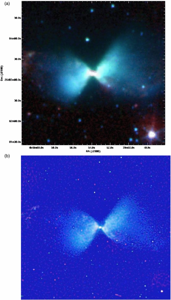
Figure 1. Example of a comparison of HiRes denconvolved Spitzer IRAC images with unprocessed mosaic images in the literature: false three-color IRAC images of L1527 (blue: 3.6 μm, green: 4.5 μm, and red: 8.0 μm). (a) unprocessed mosaic image reproduced from Tobin et al. (2008). (b) the HiRes deconvolved image.
Download figure:
Standard image High-resolution image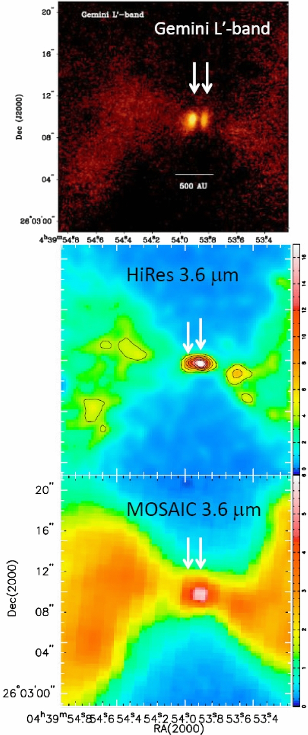
Figure 2. Spitzer 3.6 μm HiRes deconvolved image compared with a high-resolution (pixel scale of 0049) Gemini L'-band (3.8 μm) image of the outflow in L1527. For comparison, the IRAC 3.6 μm mosaic image is shown in the lower panel. Note that the subarcsecond resolution enhancement in the deconvolved image (middle panel) brings out the innermost structure, as observed in the high-resolution image in the top panel (reproduced from Tobin et al. 2010).
Download figure:
Standard image High-resolution image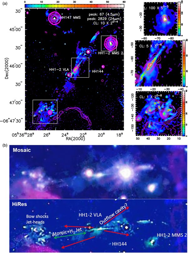
Figure 3.
Results of HiRes deconvolution of 53 Spitzer IRAC and MIPS images are presented as intensity maps in Figures 3.1–3.53. These images contain 89 protostellar objects and associated jets and outflows. Images of HH1-2 are shown here: (a) The 4.5 μm and 24 μm HiRes deconvolved images. The MIPS 24 μm image is overlaid as contours on the IRAC 4.5 μm gray scale image. A square root color stretch is used to bring out low and high brightness emissions and the contour levels are in increments of factors of two or larger as indicated. The peak intensities (in units of MJy Sr−1) in the protostar/jet-outflow are indicated. The panels to the right show blowups of the selected regions highlighted by boxes in the left panel. The atomic jet features, traced by the atomic and/or ionic line emissions within the MIPS 24 μm band are identified by the 24 μm contours overlaid on the 4.5 μm gray scale image. (b) three-color representation of HiRes deconvolved Spitzer IRAC images (lower panel): IRAC 3.6 μm (blue), 4.5 μm (green), and 8.0 μm (red). The mosaic images are shown in the upper panel. The images are re-orientated to conserve space and the orientation in the sky is easily inferred from panel (a) above. In the three-color representation the blue excess identifies the wide-angle outflows and the green excess the H2 jets and bow shocks. The H2 jets (green arrows). (The complete figure set (53 images) is available in the online journal.)
Download figure:
Standard image High-resolution imageIn the online version of this paper, we present in Figures 3.1–3.53 the results of HiRes deconvolution of Spitzer images containing 89 protostellar objects and associated jets and outflows. A list of the objects and maps are summarized in Table 1. These objects have been studied by several authors. The reference(s) in Column 6 are provided only as examples where the basic data on the object are given. In Column 7, we list the type of the input data used for HiRes processing, as discussed in Section 2.2. The last column (8) lists the figure number in which the images of the object is shown. Each HiRes image typically covers an angular size of ∼5' and may include one or more protostellar objects or jet/outflow features as listed in Table 1 and these are identified in the respective figures (Figures 3.1–3.53). The HiRes FITS data will be available at http://spitzer-outflows.jpl.nasa.gov. Our objective here is limited to presenting an overview of the deconvolved images to give a perspective on how these data could support further studies of protostellar jets and outflows. Therefore, for illustrative purposes, we only discuss one image in detail.
3.1. HH 1-2: An Example HiRes Image
Figure 3.1 is an example of how our HiRes images are displayed in Figures 3.1–3.53. In each figure, there are two panels: (a) the 24 μm emission is overlaid as contours on the 4.5 μm image and (b) an RGB three-color representation of IRAC 3.6 μm (blue), 4.5 μm (green), and 8 μm (red). We chose to display a 4.5 μm image since it traces equally well both the scattered light and H2 line emission in the jet outflow. The 24 μm emission contours identify the driving source (protostar/disk) associated with the jets and outflows. Furthermore, in cases where the atomic jet features, traced by the atomic and/or ionic line emission within the MIPS 24 μm band, are present, they are identified by the 24 μm contours overlaid on the 4.5 μm grayscale image. To highlight such features more clearly, where it is useful, we show a zoomed view of the selected regions (indicated by the boxes in the left panel) on the right-hand side of the figure. The three-color representation in the lower panel (b) helps to highlight the color differences among various features, especially the wide-angle outflow traced by blue representing the scattered light (predominantly at 3.6 and 4.5 μm) and the H2 jets/bow shocks in green and red. The protostellar object and the jet outflow features are also identified in the figures in panels (a) and (b).
HH1/HH2 is a well-studied system (the first detected HH object); see, for example, Noriega-Crespo & Raga (2012) for a detailed anatomy of the jets and counter-jets as seen in Spitzer images. These data are a good example to illustrate the significant features that can be traced in the HiRes Spitzer images. Furthermore, as far as we know, this object is the only one for which there exists a deconvolved image using other techniques. Note that the HiRes image at 4.5 μm in Figure 3.1(a) compares well with a recently deconvolved image (Noriega-Crespo & Raga 2012) obtained by using a different algorithm, the deconvolution software A WISE Astronomical Image Co-Adder (AWAIC), developed by the Wide Field Infrared Survey Explorer(WISE) for the creation of their Atlas images (see, e.g., Masci & Fowler 2009). Of particular importance in our results, as seen in the enlarged view (in the right panels in Figure 3.1(a)), is the association of 24 μm features with the optical knots in HH2 (southeast), as identified by Raga et al. (1990) and Noriega-Crespo & Raga (2012), as well as with the jet and counter jet. These 24 μm features trace the atomic and ionic jet features, as discussed in the cases of HH46/HH47 and Cep E (Velusamy et al. 2007, 2011). Another new feature in our results in Figure 3.1(b) is the detection of the wide-angle outflow cavity, implying that the protostar HH1-2 VLA is driving simultaneous wide-angle outflow and collimated jets.
As reported in the case of Cep E (Velusamy et al. 2011), the MIPS images have small pointing differences (∼1'') with respect to the IRAC images. This offset is also evident in some of the maps shown Figures 3.1–3.53. The difference in the positions of the point sources between the IRAC and MIPS images is, in part, due to the fact that MIPS used a scan mirror to change the field of view during their observations and the mechanism itself suffered a hysterisis effect that increased the positional uncertainty by 06–10. This uncertainty is a small fraction of the MIPS beam at 24 μm in the mosaic images, but it becomes more obvious when comparing MIPS and IRAC HiRes images. Note that the MIPS images shown in the figures or the FITS image data are not corrected for any pointing offset with respect to the IRAC images. Therefore, in case detailed positional matching is required, the pointing offset can be obtained by comparing the "point" sources in the MIPS 24 μm image with their counterparts in the IRAC bands using the HiRes FITS images. The MIPS handbook gives a 1σ radial uncertainty of 14, compared with ∼02 for IRAC.
One problem with HiRes deconvolution is that it tends to resolve out very smooth, extended low surface brightness features. Optimal-performance HiRes requires that the background emission is fully subtracted out in each BCD prior to applying the deconvolution. Furthermore, the positivity criteria implicit in the deconvolution algorithm makes it insensitive to negative intensities. In rare cases (as in Figure 3.53), although the HiRes-deconvolved image is free from side lobe contamination from bright sources in the image, its resolution enhancement and its lack of preserving the background can make it harder to detect extremely extended low surface brightness emission.
3.2. Summary of Spitzer HiRes Images
Figures 3.1–3.53 highlight the prominent features in the HiRes images of the protostar regions. The HiRes FITS images contain more details over the full extent of the processed maps and will be available in the Web site given above. Spitzer's coverage of a broad range of infrared emission in the IRAC and MIPS bands with high sensitivity and photometric stability, along with the IRS data in some cases, provides sufficient information for a comprehensive modeling of the spectral energy distribution (SED) to derive the physical characteristics and the evolutionary stages of protostars (cf. Robitaille et al. 2007; Forbrich et al. 2010). However, by applying the HiRes reprocessing, we can extract even more information from the Spitzer data. As demonstrated in Figure 3.1, the sensitivity, the resolution enhancement, and removal of the diffraction lobe confusion have led to visualizing and characterizing more clearly the following.
- 1.Very high dynamic ranges in the maps in which the protostar is well resolved on a subarcsecond scale from the surrounding jets and outflows.
- 2.The protostar-disk itself is detectable in the IRAC bands in many cases (with relatively low obscuration) and almost always in the MIPS bands.
- 3.Wide-angle outflow cavities in the IRAC 3.6 and 4.5 μm images are identified by the scattered photospheric starlight; although they are visible in the Mosaic standard pBCD products, they are brought out more clearly in the HiRes images.
- 4.Jets and bow shocks in H2 molecular emission within the IRAC bands.
- 5.The hottest atomic and ionic gas in the jet and jet head traced by the [Fe ii]/[S i] line emission within the MIPS 24 μm band.
The Spitzer IRAC and MIPS bands offer a unique resource to study a wide range of components simultaneously: protostars, protostellar disks, outflows, protostellar envelopes, and cores. At the short-wavelength IRAC bands, the outflow cones are observable in scattered light from the protostar through the cavity created by the jets and outflows (cf. Tobin et al. 2007; Velusamy et al. 2007, 2011). A significant fraction of the emission in the IRAC bands is also considered to contain emission from the H2 rotational lines (e.g., Noriega-Crespo et al. 2004a, 2004b; Smith & Rosen 2005; Neufeld & Yuan 2008) and therefore is an excellent tracer of H2 emission in the protostellar jets. Recently, Velusamy et al. (2007, 2011) have shown that molecular jets and molecular gas in the bow shocks are readily identifiable in the IRAC bands, while the hottest atomic and ionic gases in the bow shocks are also identifiable in the MIPS 24 μm band, which covers a few atomic and ionic emission lines. The dust emission from the protostar in the MIPS bands is a good diagnostic of the circumstellar disks.
With the exception of HH 1-2 MMS 3, all the other protostars are detected in one or more bands in the processed images. In at least three cases, BHR 71, CG 30, and CB 230, we clearly detect the binary components and associated H2 jets and outflows. The binary components (A,B) in L1448 IRS3 (cf. Tobin et al. 2007), IRAS 16293-2422 (cf. Takakuwa et al. 2007), and L723 (cf. Girart et al. 2009) are marginally to well resolved in the 24 μm HiRes images. We clearly detect 31 wide-angle outflows in scattered light in the IRAC bands (there may be others that are less obvious due to confusion with other features). Out of these, there are 12 outflows, including B5 IRS1, which is known to have parsec-scale HH flows (Yu et al. 1999), in which no detectable H2 jets or bow shocks have been observed. In about 14 H2 jet/bow-shock systems, atomic/ionic emission in the jet/jet heads is detected in the MIPS 24 μm images. Prominent atomic jets are evident, for example, in Figures 3.1 (HH 1-2), 3.16 (HH 211), 3.30 (HH 92), 3.31 (HH 212), 3.37 (HH 46/47) 3.42 (Serp-SMM1), and 3.52 (Cep E).
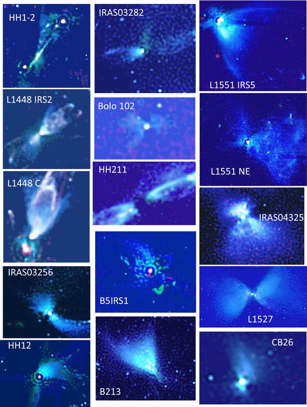
Of the wide-angle outflows, 31, representing a large fraction of the sample, show a high efficiency of scattered light in the Spitzer images as a tracer of outflow cavities. In Figure 4, we show an image gallery of all 31 outflows. Although the wide-angle outflows are observed by their CO emission, a comparison between the outflow cavities traced in the Spitzer images of HH46 and in the ALMA maps of CO emission show that the former is broader than the latter (Arce et al. 2013). In the case of CB 26 (Launhardt et al. 2008), a narrower outflow is also detected in CO than is seen in the scattered light cavity. Arce et al. argue that the narrower outflow seen in 12CO is a consequence of opacity effects. In Figures 5 and 6, we show two examples of a comparison between the Spitzer scattered light cavity and the CO outflows. In the case of L 483, shown in Figure 5, we overlay the redshifted and blueshifted 12CO (1-0) intensity contours on the HiRes Spitzer image at 4.5 μm (see Figure 3.41). The 12CO (1-0) maps are from our unpublished OVRO observations made in 1997. The redshifted lobe is narrower than the blueshifted lobe and both show narrower opening angles compared with those in scattered light. The narrower opening angle for the CO outflow may be evidence for 12CO opacity effects close to the source. In the second example shown in Figure 6, we compare the scattered light in the HiRes Spitzer image at 4.5 μm of Cep E (left panel) with the OVRO 13CO (1-0) maps (right panel) obtained by Moro-Martín et al. (2001). Clearly, the 13CO outflow seems to trace the full extent of the scattered light cavity (also shown in Figure 3.52), as may be expected for 13CO, which has a lower opacity compared with 12CO in the previous example. Thus, compared with CO, the Spitzer images offer a more powerful tool to study the morphology of wide-angle outflows detected in scattered light. In addition to the scattered light cavities, the H2 molecular jets, bow shocks, and, in some cases, the atomic/ionic jet components, when present, are also detected in the Spitzer images, thus providing a more complete morphology of the protostellar outflows and jets. The predominance of the simultaneous presence of collimated jets and wide-angle outflows in our sample (19 out of 31) is consistent with unified jet outflow models such as those presented by Machida et al. (2008) in which the accretion in the compact protostellar disk drives the high-velocity jets and the accretion from the extended infall envelope drives the wide-angle outflows.
Download figure:
Standard image High-resolution image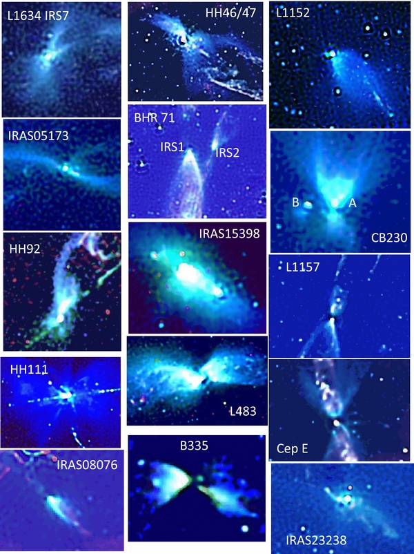
Figure 4. Image gallery of all 31 wide angle outflows observed in the HiRes processed Spitzer sample: three-color IRAC HiRes image with 3.6 μm (blue), 4.5 μm (green), and 8.0 μm (red). The wide angle cavities are identified by the color excess (blue). Note B5 IRS1 and HH12 have large side-lobe residue due to saturation. Fifteen outflows are shown here and remaining 16 are shown in 15 panels on the next page.
Download figure:
Standard image High-resolution image
Figure 5. L483: comparison of the scattered light outflow cavity traced in HiRes 4.5 μm image with 12CO(1-0) outflow lobes. CO outflow intensity contours (at interval 0.4 Jy beam−1) overlaid on the 4.5 μm image. Red and blue contours represent the red-shifted (Vlsr = 6.5 – 10.4 km s−1) and blue-shifted (Vlsr = 0.0 – 3.9 kms−1) lobes respectively. The rest Vlsr is 5.2 km s−1. The CO data are from our OVRO observations with a synthesized beam of 4.6'' × 3.3''. The arrows mark the outflow cavities as traced by the scattered light at 4.5 μm and CO emissions.
Download figure:
Standard image High-resolution image
Figure 6. Cep E: comparison of the scattered light outflow cavity traced in the HiRes 4.5 μm image with 13CO(1-0) outflow lobes. Left: 4.5 μm image. Right: contour map of CO outflow intensities of the red-shifted and blue-shifted lobes observed with the OVRO (reproduced from Moro-Martín et al. 2001). The arrows mark the outflow cavity traced by the scattered light at 4.5 μm.
Download figure:
Standard image High-resolution imageOur sample contains a large number of H2 jet/bow shocks (partly due to the selection of many known HH objects). The data presented here provide a comprehensive database to study the number, distribution, and their separation from the protostar of the H2 knots and bow-shocks, which are indicators of the episodic ejections and/or the inhomogeneities in the surrounding interstellar medium.
3.3. Time Evolution of Outflow Morphology
Protostellar jets and outflows carve cavities and inject energy, momentum, and turbulence into the surrounding medium (e.g., Shu et al. 2000; Bally 2007). They have a profound effect on the parent core, which is the reservoir for material accreted by the forming star, and thus on the final properties of the newborn star as well. Outflows originate close to the surface of the forming star (e.g., Pudritz et al. 2007) and such a clearing out of the gas and dust along with a widening of the outflow with time can lead to the termination of the infall phase (Velusamy & Langer 1998). A possible evolutionary trend in the outflow morphology (widening with time) as a function of age was seen in a sample observed in CO (Arce & Sargent 2006) and is predicted in the simulations of outflow evolution (Offner et al. 2011). A broadening of outflow with age was also found by Seale & Looney (2008), who used the scattered light in the outflow cavities in the unprocessed Spitzer images of 27 young stellar objects combined with their SEDs to quantify the shapes of the outflow.
In Table 2, we list all 31 of the wide-angle outflows detected in our sample (see Figure 4), along with the opening angles measured, as discussed below. The outflow shapes are typically parabolic; the opening angles are the broadest at the base and narrower at larger distances from the vertex of the cavity. As discussed in Velusamy & Langer (1998), to study the evolution of the outflow, the opening angle measured near the base is most relevant. When bipolar outflows are clearly seen, we use only the widest lobe for measuring the opening angle. We do not use the average of the opening angles of the outflow and the counter outflow because, in addition to the evolutionary status of the outflow, its observed characteristics may vary with the viewing geometry (inclination) and/or the environmental conditions of the protostellar and circumstellar envelopes. For the purpose of tracing the outflow evolution with age, the most critical outflow characteristic is the opening angle near the vertex, at the start of the outflow (cf. Velusamy & Langer 1998) before it is modified by any environmental effects. Therefore, we can assume that the widest opening angle in any of the lobes is the most representative of the opening angle for correlating with age. The opening angles are not corrected for inclination and are listed in Column 2 of Table 2. Note that the arrows marked in Figures 3.1(b)–3.53(b) are meant to draw attention to the presence of wide-angle outflow and they do not represent the exact opening angles. The values of the opening angles in Table 2 are measured between the boundaries of the widest outflow lobe in each object.
Table 2. Opening Angle of Wide-angle Outflow Cavities
| Primary Name | Opening | Tbol | Ageb | |
|---|---|---|---|---|
| Angle(deg)a | (K) | Ref. | (103 yr) | |
| L1641 VLA1 | 50 | 41 | 1 | 0.9(0.2, 3.7) |
| L1448-IRS2 | 70 | 43–63 | 2 | 2.6(0.7, 10.4) |
| L1448 C (N) | 65 | 49–69 | 2 | 3.3(0.8, 13.0) |
| HH12 | 100 | 304 | 2 | 115(29, 456) |
| IRAS 03256+3055 | 100 | 67 | 2 | 3.0(0.8, 12.1) |
| IRAS03282+3035 | 80 | 33–60 | 3 | 1.3(0.3, 5.2) |
| Bolo 102 | 95 | 72 | 2 | 3.6(0.9, 14.4) |
| HH 211-MM | 50 | 24 | 2 | 0.3(0.1, 1.0) |
| B5 IRS1 | 130 | 287 | 2 | 100(25, 397) |
| B213 | 80 | 72 | 2 | 3.6(0.9, 14.4) |
| L1551-IRS 5 | 105 | 92 | 4 | 6.5(1.6, 25.9) |
| L1551-NE A/B | 100 | 91 | 4 | 6.3(1.6, 25.2) |
| IRAS 04325+2402 | 110 | 73 | 4 | 3.7(0.9, 14.9) |
| L1527 | 98 | 56 | 4 | 2.0(0.5, 7.9) |
| CB26 | 115 | 770 | 5 | 1065(268, 4242) |
| L1634 IRS7 | 76 | 64c | 6 | 2.7(0.7, 10.8) |
| IRAS 05173−0555 | 64 | 58c | 6 | 5.7(1.4, 22.6) |
| HH92 | 60 | 41c | 7 | 0.9(0.2, 3.7) |
| HH111MMS | 118 | 78 | 4 | 4.4(1.1, 17.4) |
| IRAS 08076−3556 | 42 | 117 | 4 | 0.7(0.2, 2.9) |
| HH46/47 | 110 | 40–145 | 8 | 19.4(4.9, 77.1) |
| BHR71-IRS1 | 45 | 44 | 9 | 1.1(0.3, 4.4) |
| BHR71-IRS2 | 42 | 58 | 9 | 2.1(0.5, 8.6) |
| IRAS1 5398−3359 | 120 | 48–61 | 4 | 2.4(0.6, 9.7) |
| L483 | 70 | 50–54 | 3 | 1.8(0.5, 7.2) |
| B335 | 63 | 28–45 | 3 | 1.2(0.3, 4.7) |
| L1152 | 64 | 48c | 6 | 1.4(0.3, 5.4) |
| L1157 | 54 | 40–60 | 3 | 1.0(0.2, 3.9) |
| CB230 | 95 | 69 | 4 | 3.3(0.8, 13.0) |
| CepE-MM | 85 | 56 | 4 | 2.0(0.5, 7.9) |
| IRAS 23238+7401 | 98 | 64c | 6 | 2.7(0.7, 10.8) |
Notes. aThis paper. b1σ lower and upper limits are given in parentheses. cEstimated from the SED peak. References. References for Tbol: (1) Fischer et al. 2010; (2) Enoch et al. 2009; (3) Chen et al. 2013; (4) Froebrich 2005; (5) Stecklum et al. 2004; (6) Seale & Looney 2008; (7) Miettinen & Offner 2013; (8) Emerson et al. 1984; (9) Chen et al. 2008.
Download table as: ASCIITypeset image
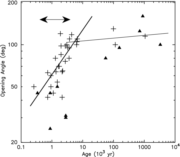
Following the approach of Arce & Sargent (2006), we use Tbol as a measure of the protostellar age. In Table 2, we list the values for Tbol collected from the literature, as indicated in Column 3. When a range of values are given, we use their mean value for estimating the ages. In a few cases, we estimated the Tbol values using the SEDs available in the literature and these are noted in the table. The ages were estimated from Tbol using the empirical relationship given by Ladd et al. (1998) in their Appendix (Equation (C9)). The ages and their uncertainties are listed in Column 5 in Table 2. The uncertainty in the estimated ages corresponds to the uncertainty in the empirical fit, as given by Ladd et al. In Figure 7, we show the plot of opening angle versus protostellar age for all 31 outflows in our sample (denoted by crosses). The uncertainty in the ages is also indicated. The error in the measured opening angles is small (<5°). We also included in this plot the data from Arce & Sargent (2006) represented by filled triangles. The scatter in this plot is large, but a trend in the opening angle, increasing with age, is evident. For example, we can fit power laws as shown in Figure 7: opening angle, θ(deg) = 6.7×[t(yr)]0.32 for ages <8000 yr and θ(deg) = 88.5×[t(yr)]0.02 for ages >7000 yr. (For the fits, we use only the data in our sample, all observed by scattered light in the processed Spitzer images). At ages ⩾ 8000 yr, the plot suggests a slower rate for the increase of opening angle with time, which would be consistent with the opening angles approaching 180° asymptotically. The scarcity of data at higher ages is due to the fact that our sample is primarily Class 0 objects with just two Class 1 objects (B5 IRS1 & HH46/47). It should be noted that we do not correct the opening angle for inclination. Although a widening trend is evident in our data, any interpretation of fit to the data is subject to the large uncertainty in their ages.
Figure 7. Age vs. the opening angle of all wide angle outflows detected in the HiRes images. The crosses (+) are data from the present sample, used for the power law fits. The power law fits, for opening angle versus age, are shown for ages <8000 yr (thick line) and for ages >7000 yr (thin line) have exponents 0.32 and 0.02 respectively. Filled triangles are data from Arce & Sargent (2006) which are not used for the fit. The double arrow indicates the uncertainty in the age estimate.
Download figure:
Standard image High-resolution image
Our results are broadly consistent with the plots in Arce & Sargent (2006) and Seale & Looney (2008). However, our values for the opening angles seem higher than those in their results. The "intensity weighted" opening angles estimated by Seale & Looney using azimuthal intensity in their circular cuts are also likely to be narrower than those measured geometrically from high spatial resolution images. Arce & Sargent used CO outflow data. Due to opacity effects, the 12CO may not trace the entire extent of the outflow cavity, as opposed to scattered light (Figure 5; also see Arce et al. 2013). Thus, the data from the HiRes processed images clearly provide the most consistent set of apparent opening angles for the entire extent of the cavity. Nevertheless, the observed trend in the opening angle versus age is subject to the large uncertainties in estimating the ages. Reliable age estimates combined with a more detailed characterization of the morphological shape of the cavity should provide observational constraints on the theories of outflow and star-formation processes.
4. SUMMARY
By combining the high sensitivity of Spitzer images and reprocessing with HiRes deconvolution on a large sample of protostellar objects, we show that the jet and outflow features are more easily identified than those in the Spitzer mosaic images alone. These features include (1) wide-angle outflow seen in scattered light, (2) morphological details of jet-driven bow shocks and jet heads or knots, and (3) compact features in 24 μm image identified as atomic/ionic line emission within the MIPS band coincident with the jet features. The maps and the FITS image data presented here can be used to study these protostellar components in detail, as demonstrated in the case of Cep E (Velusamy et al. 2011). We can study directly the scattered light spectrum and hence the protostellar SED in deeply embedded protostars, by separating the protostellar photospheric scattered emission in the wide-angle cavity from the jet emission. The high contrast resolution-enhanced images in the Spitzer HiRes sample provide a robust description of the morphology of the wide-angle outflow cavity in 31 objects. A trend for a widening of the opening angle with age is evident in the power-law fits to these data. We can obtain the H2 emission line spectra as observed in all IRAC bands for the knots and use their IRAC colors as probes of the temperature and density in the jets and bow shocks. Such spectra are useful as diagnostics of the C-type shock excitation of pure rotational transitions of H2 and a few H2 vibrational emission within each IRAC band. Detailed modeling of the individual shocks will help retrace the history of episodic jet activity and the associated accretion onto the protostar. Our resolution-enhanced Spitzer image data on such a large sample of protostellar objects will be a resource to future studies of these objects. It is encouraging to see that in addition to our algorithm developed for Spitzer images, newer ones such as the deconvolution software AWAIC are becoming available. The results presented in this paper support the usefulness and the need for reprocessing with deconvolution techniques the protostellar data obtained by high sensitivity but low spatial resolution observations in Spitzer, Herschel, and WISE surveys.
We acknowledge Dr. C. A. Beichman for suggesting the development of the HiRes deconvolution tool for Spitzer images. We also thank the referee for helpful suggestions. This publication makes use of the Protostars webpage hosted by the University of Kent. This ADAP (ROSES 2009)-sponsored research was conducted at the Jet Propulsion Laboratory, California Institute of Technology under contract with the National Aeronautics and Space Administration. In 1997, the Owens Valley Radio Observatory millimeter array, which we used to observe CO, was supported by the National Science Foundation grant number AST-96-13717 ©2013. All rights reserved. California Institute of Technology: USA Government sponsorship acknowledged.
Footnotes
- *
FITS images available at http://spitzer-outflows.jpl.nasa.gov.